

Abstract
Background:
Lung cancer is the deadliest and second most common cancer in the United States due to the lack of symptoms for early diagnosis. Pulmonary nodules are small abnormal regions that can be potentially correlated to the occurrence of lung cancer. Early detection of these nodules is critical because it can significantly improve the patient’s survival rates. Thoracic thin-sliced Computed tomography (CT) scanning has emerged as a widely used method for diagnosing and prognosis lung abnormalities.
Purpose:
The standard clinical workflow of detecting pulmonary nodules relies on radiologists to analyze CT images to assess the risk factors of cancerous nodules. However, this approach can be error-prone due to the various nodule formation causes, such as pollutants and infections. Deep learning algorithms have recently demonstrated remarkable success in medical image classification and segmentation. As an ever more important assistant to radiologists in nodule detection, it is imperative ensure the deep learning algorithm and radiologist to better understand the decisions from each other. This study aims to develop a framework integrating explainable AI methods to achieve accurate pulmonary nodule detection.
Methods:
A robust and explainable detection framework is proposed, focusing on reducing false positives in pulmonary nodule detection. Its implementation is based on an explanation supervision method, which uses nodule contours of radiologists as supervision signals to force the model to learn nodule morphologies, enabling improved learning ability on small dataset, and enable small dataset learning ability. In addition, two imputation methods are applied to the nodule region annotations to reduce the noise within human annotations and allow the model to have robust attributions that meet human expectations. The 480, 265, and 265 CT image sets from the public LIDC-IDRI dataset are used for training, validation, and testing.
Results:
Using only 10, 30, 50 and 100 training samples sequentially, our method constantly improves the classification performance and explanation quality of baseline in terms of AUC and IoU. In particular, our framework with a learnable imputation kernel improves IoU from baseline by 24.0% to 80.0%. A pre-defined Gaussian imputation kernel achieves an even greater improvement, from 38.4% to 118.8% from baseline. Compared to the baseline trained on 100 samples, our method shows less drop in AUC when trained on fewer samples. A comprehensive comparison of interpretability shows that our method aligns better with expert opinions.
Conclusions:
A pulmonary nodule detection framework was demonstrated using public thoracic CT image datasets. The framework integrates the robust explanation supervision technique to ensure the performance of nodule classification and morphology. The method can reduce the workload of radiologists and enable them to focus on the diagnosis and prognosis of the potential cancerous pulmonary nodules at the early stage to improve the outcomes for lung cancer patients.
Keywords: Explainable AI, Pulmonary nodule detection, Deep learning
1. Introduction
According to the American Cancer Society, lung cancer is the deadliest and second most common cancer in the United States. Pulmonary nodules are small abnormal regions that can potentially be correlated to a sign of lung cancer. Early detection of these nodules can increase the patient’s survival rate from lung cancer1 early treatment. Computed tomography (CT) has been widely used for nodule diagnosis and prognosis via thoracic scanning protocol that provides sufficient spatial resolutions to detect the abnormalities of the lung2. Radiologists can analyze the thoracic CT images and forecast the risk factors of cancerous nodules. However, pulmonary nodules can be caused by abnormal growth of cells, pollutants, autoimmune diseases, fungal infections, respiratory system infections, and scar tissues. The complexity of nodule formation increases the workload of radiologists and the uncertainty of human factors to miss the diagnosis of lung cancerous nodules at the early stage3. Recently, deep learning (DL) algorithms have shown great success in medical applications regarding classification4–6 and segmentation7–9. This work aims to propose a framework that leverages the state-of-the-art explainable AI methods10,11 to increase the accuracy of pulmonary nodule detection.
DL has been implemented into clinical radiation treatment planning for organ segmentation; for instance, the U-Net12 is one of the most popular models recognized through international conferences13–15. Conventional model architectures, such as residual networks, can also achieve good segmentation results in clinical applications by integrating multi-modality and multi-level contextual information16. The success of these DL models raises the motivation to use computer-aided detection (CAD) systems to assist radiologists in nodule delineation. To effectively detect nodules from thoracic CT scans, two fundamental challenges need to be overcome: (a) the variety of nodule morphology leads to difficulties in identification; (b) the lack of interpretability leads to unconvincing or agnostic reasoning processes, limiting clinical translation17. The first issue has been widely explored18–21 for lung nodules with various geometrical features. While most current CAD-based nodule detection systems merely focus on exploiting the information from CT images, it has yet to be widely investigated how to leverage the rich information from physician nodule contours. As for the second issue, the development of model interpretability is still in its infancy.
Inspired by Explainable AI22–25 techniques, human-understandable explanations in DL models have become a promising solution to interpretable CAD systems. One mainstream explanation tool is to visualize where the model “sees”.26,27 This approach generates an attention map indicating which part of the input is responsible for the model prediction. Based on an explanation tool, explanation supervision technique integrates expert opinions in the DL model to make it more focused on the lung nodule regions. Expert opinions can be expressed through explanation annotations, which can inform the model where to look for potential cancer nodules. Such a technique synthesizes both images and explanation annotations to supervise the model training28. Linsley et al29. Demonstrated how to use the explanation annotations to give accurate predictions that are in line with human expectations. Mitsuhara et al30 implemented explanation supervision technique to customize an attention-branching network31 to enhance image prediction. Several recent studies32,33 have shown that explanation supervision techniques can be flexibly implemented into various DL models. However, medical experts’ opinions are noisy compared to mathematical formulas and may bias the DL model, returning physically unreasonable outcomes. For example, different radiologists may have different contours of the nodule’s margins, and the contoured region of the nodule may be inaccurate.
RES (Robust Explanation Supervision)34 is a generic framework for guiding visual explanation that allows DL models to be trained using even noisy annotations. For example, inaccurate nodule contours will be imputed based on a prior about the inaccuracy. In this work, we leverage the RES method in our proposed nodule detection framework to enhance DL-based pulmonary nodule detection by reducing false positives. Our framework, called RXD (Robust and eXplainable Detection), can enable robust and explainable pulmonary nodule identification by leveraging expert knowledge of contours while reducing the inaccuracy of human annotations. Another factual issue to consider is that the amount of data available is usually scarce. Previous studies35,36 had exhibited that small dataset learning was achievable by integrating expert opinions into DL training. This work also explores the feasibility of using the proposed nodule detection framework for small dataset learning.
2. Materials and methods
2.1. Dataset
We used a nonproprietary dataset37–39, the Lung Image Database Consortium and Image Database Resource Initiative (LIDC-IDRI) dataset, to evaluate the proposed pulmonary nodule detection framework. The LIDC dataset are one of the most common multi-institute datasets for lung nodule detection used by many previous investigations40–42. The dataset includes thoracic CT scans from 1,010 patients with slice thickness ranging from 0.6 to 5.0 mm, acquired from seven academic centers and eight medical imaging companies. The CT scanners included GE Medical Systems LightSpeed Plus, Philips Brilliance, Siemens Definition, Emotion, and Sensation scanner models, and Toshiba Aquilion. The CT images were acquired by using single energy scans including spectrum energies of 120 kV, 130 kV, 135 kV, and 140 kV with the mean tube current of 222 mA. The CT slice thicknesses were ranging from 0.6 mm to 5.0 mm, and the mean pixel width was 0.688 mm. Due to the involvement of multiple CT scanners, the reconstruction kernels varied among vendors, but all images were acquired based on the thoracic protocols. Four experienced radiologists adequately evaluated the thoracic CT images via a two-stage process to ensure precise and accurate nodule annotations. At the first stage, each radiologist independently reviewed the images and classified the lesions into three categories (nodules ≥3 mm, nodules <3 mm, and non-nodules). Based on previous work43, the concept of a nodule might not encompass a singular entity that can be easily defined, and LIDC Research Group44 defined these three categories to impose different requirements for radiologists to characterize nodules regarding shape, lobulation, margin, and likelihood of malignancy45. Then the most likely nodule contours were concluded from the best knowledge from all radiologists. In this work, we aim to use the data for the nodule detection purpose, and we classified positive and negative data for images with and without nodules.
2.2. Data preparation
This work consisted of 1,010 CT image sets from 1,010 patients with total image slices of 68,130. Patients’ CT image sets were randomly sampled (without resampling) into training, validation, and testing that included 480, 265, and 265 CT image sets, which contains 55,755, 6,507, and 5,868, CT image slices, respectively. We used patch-based training with the bounding boxes for nodule contour annotations. For the nodule annotations, a typical 50% consensus consolidation of radiologist annotations was performed to reflect that the ground truth nodule regions were agreed by at least two radiologists. Then, the bounding boxes of nodule contour annotations were spatially extended by 20 pixels to obtain the corresponding image blocks. The CT images that contain the image blocks are positive samples, while the remaining images are negative samples. Imagine a Rubik’s cube, the center of which is an image block containing a nodule, and the axial slices of the other 26 blocks were extracted as negative samples. Blocks that exceed the image boundaries are discarded. As a result, 2,625 positive samples and 65,505 negative samples were obtained, which is an extremely imbalanced dataset. A balancing strategy was involved in training to mitigate the impact of imbalance, while the original proportions were maintained in validation and test sets to simulate the real-world situation. The balancing strategy uses the patient IDs of the positive samples to draw the same number of negative samples as the positive ones. Table 1 shows the data distribution of the training set, validation set and test set. To build a truly robust CAD system, we considered all samples to be available with no restrictions on the thickness of the slices. All samples were normalized between 0 and 1, and then converted to PNG format for ease of use.
Table 1.
Data distribution of the training set, validation set and test set. The training set was balanced, while validation and test sets maintained the original proportions.
| Training set | Validation set | Test set | |
|---|---|---|---|
| Positive samples | 50% | 4% | 4% |
| Negative samples | 50% | 96% | 96% |
The axial slice of each nodule contour annotation was used as a human explanation annotation. Typically, explanation supervision requires human explanation annotations for both positive and negative samples to guide the model where to attend. However, there is no such annotation for negative samples in the LIDC-IDRI dataset. As a further incentive for the model to learn to distinguish between positive and negative samples, we generated an explanation annotation for each negative sample with the same shape as the negative sample, all with a value of 0 (given that the human explanation annotation for the nodule region has a value of 1). Figure 1 shows examples of positive and negative samples, along with the corresponding explanation annotations. All image patches and nodule region annotations of positive samples were obtained with the help of pylidc46 package.
Figure 1.
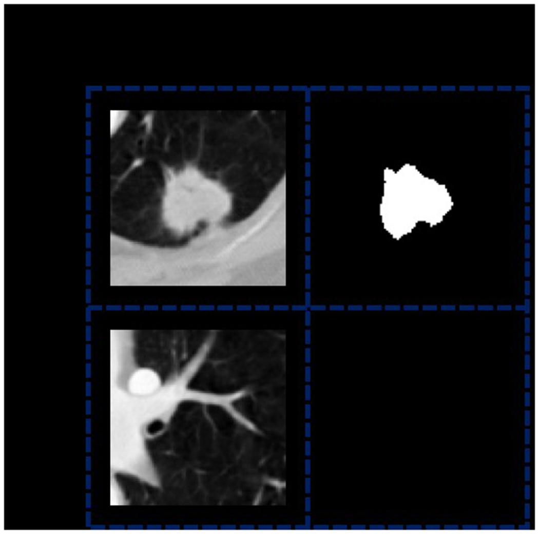
Examples of positive and negative samples, along with the corresponding explanation annotations. The explanation annotation of the positive sample is a black and white mask, where the white region represents the nodule region, which has a value of 1 at each pixel. The black region represents the non-nodule region, which has a value of 0 at each pixel. As a comparison, the explanation annotation of the negative sample is a black mask with a value of 0 for each pixel.
2.3. Methods
2.3.1. Robust explanation supervision for pulmonary nodule detection
We considered the pulmonary nodule detection task as a two-dimensional (2D) image classification task since physicians’ contours were based on transversal CT image slices. This nodule detection problem can be formulated as: suppose is a 2D slice with channels, height and width , and is the class label of , where 1 denotes positive and 0 denotes negative. A deep neural network (DNN) should learn the mapping function from each to its label .
Each positive sample in the LIDC-IDRI dataset initially contains nodule contour annotations from four radiologists, which can provide abundant information about nodule contour and location. A natural idea is to exploit these nodule contour annotations to improve the training effect. This can be achieved by using explanation supervision technique, which incorporates explanation annotations (i.e., these nodule contour annotations) into supervision signal, improving both classification performance and inference attribution34. However, to our knowledge, no one has applied explanation supervision to clinical diagnosis, leaving the wealth of information in explanation annotations untapped. RES is a framework that utilizes explanation annotations to improve both the performance and the explanation quality of backbone DNN. To achieve this, a robust explanation loss term is introduced into its overall loss function as follows:
| (1) |
where denotes the prediction loss, which is the cross-entropy loss in this work. In the second loss term, denotes the model explanation generated for the sample using the given explanation method; denotes the explanation annotations for the sample. Since the explanation annotations are different for positive and negative samples, is further represented by a combination of two types of binary explanation annotations as follows:
| (2) |
where denotes the non-nodule lesion annotations of negative samples, denotes nodule region annotations of positive samples and denotes their consensus level. Typically, is set to 50%, meaning that a pixel is considered within the nodule region if it is included in annotations of at least two radiologists. For the positive sample, if the pixel at coordinate is within the nodule region, it is assigned (i.e., ); otherwise, it is assigned (i.e., ). For the negative sample, the pixel at coordinate is assigned (i.e., ) because non-nodule lesions are not annotated in the LIDC-IDRI dataset. The hyper-parameter is used to adjust the impact of the explanation loss, thus the baseline can be seen as a special case of RES when is equal to 0. In this work, is set to 0.05 based on grid search via classification performance on the validation set. Now, we further specify the robust explanation loss term . First, assume that the ideal model explanation generated for the sample be in the range , given that:
| (3) |
where and denote the ideal nodule region annotations of positive samples and non-nodule lesion annotations of negative samples, respectively. However, due to the potential inaccuracy of human nodule region annotations, remains unknown. Moreover, non-nodule lesions in negative samples are not annotated in the LIDC-IDRI dataset, resulting in being unknown either. Therefore, a hyper-parameter is introduced to represent the assumption about the discrepancy between and . The difference between and is measured by the L1 loss function followed by a normalization function , which divides the L1 loss by the non-zero area of the explanation annotations. The L1 loss was used to ensure the robustness of training attention-based deep learning models33. Then, the modified is as follows:
| (4) |
based on the sensitivity analysis of hyper-parameter on LIDC-IDRI dataset in the following section, is set to 0.003. With the assumption about ideal nodule and non-nodule distributions made, is then further extended to learn from noisy human explanation annotations. To measure the absolute difference between the continuous and the binary , , hyperbolic tangent function together with a slope controller is applied to binarize :
| (5) |
where is set to 5 and is the threshold value, obtained by an efficient adaptive threshold searching algorithm. A distance function is also applied to measure their relative distance:
| (6) |
where is a mapping function with kernel that maps and to continuous values in the range [0, 1]. By switching kernels, different imputations are performed for the boundaries of human explanation annotations. The is the L1 loss function because it is more robust.33 In addition, an indicator function is added to force the model to learn only from the annotated regions. To summarize, the final is as follows:
| (7) |
where is the given model parameter.
2.3.2. Framework formulation
Figure 2 depicts the structure of the proposed pulmonary nodule detection framework. The DNN model within the proposed framework can be trained using the explanation loss function defined in Eq. (7) with different kernel functions. The proposed framework using DNN models trained with a pre-defined Gaussian kernel and a learnable kernel are denoted RXD-G and RXD-L, respectively. RXD-G and RXD-L allow the underlying deep learning models and kernel functions to learn from the estimated version of the node annotations, thus reducing the chance of being misled by noise in the annotations. The proposed framework implemented RXD-G and RXD-L to explore which kernel functions can work adequately with DNN to achieve the nodule detection task. Ultimately, the model not only has high predictive power, but also generates a prediction basis that is more consistent with that of the radiologist. The commonly used ResNet1847 is used as the backbone DNN model. The overall model structure is shown in Figure 2(b). No structural changes are required for RXD-G, while RXD-L adds an imputation layer at the bottom of the backbone DNN. The imputation layer is a convolutional layer for estimating the ideal nodule region by binary nodule region annotations, converting it to a continuous value in the range [0, 1].
Figure 2.
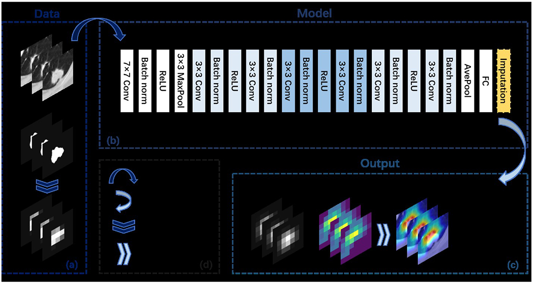
Overview of the RXD framework. Subfigure (a) illustrates the input data, which includes 2D image slices and nodule region annotations. For RXD-L, the input annotations are of the original shape (i.e., 224 × 224); while for RXD-G, the input annotations need to be down sampled first. Eventually, RXD-L and RXD-G produce attention maps with the size (i.e., 7 × 7). Subfigure (b) shows the overall model architecture when the backbone model is ResNet18. Subfigure (c) shows the output including the intermediate results (imputations and attention maps) of the model. In the case of RXD-L, the imputation is an annotation processed by the imputation layer. In the case of RXD-G, the imputation is an annotation processed by the Gaussian kernel. The attention map is produced by Grad-CAM (described in Section 2.3.3) and can be used to generate visualizations. Subfigure (d) contains symbol descriptions.
2.3.3. Deep neural network training
Existing methods for reducing false positives use only the information in the image, while both the image and the explanation annotation are used in explanation supervision. To generate model explanations that are comparable to human annotations, the widely used Grad-CAM27 was used as the explanation technique. The model explanations generated via Grad-CAM were normalized to [0, 1], by dividing the maximum attention value for each sample. As shown in Figure 2, all images were resized to 224 × 224 to fit the backbone model (i.e., ResNet18 in this work), resulting in a 7 × 7 attention map. Then, the attention map was used to calculate the explanation loss with the corresponding explanation annotation, which was down sampled to the same size as the attention map. In this way, we can avoid distorting the original model explanation when scaling up. In the same sense, for visualization and explanation quality evaluation, we took the opposite approach: scaling up the attention map to the same size as the explanation annotation. In the process of calculating the explanation loss in RES, explanation annotations need to be imputed and converted to continuous values. Due to the differences in implementation, RXD-G imputes the explanation annotations after down sampling, while RXD-L imputes the original annotations. Figure 3 illustrates their different ways of imputation.
Figure 3.
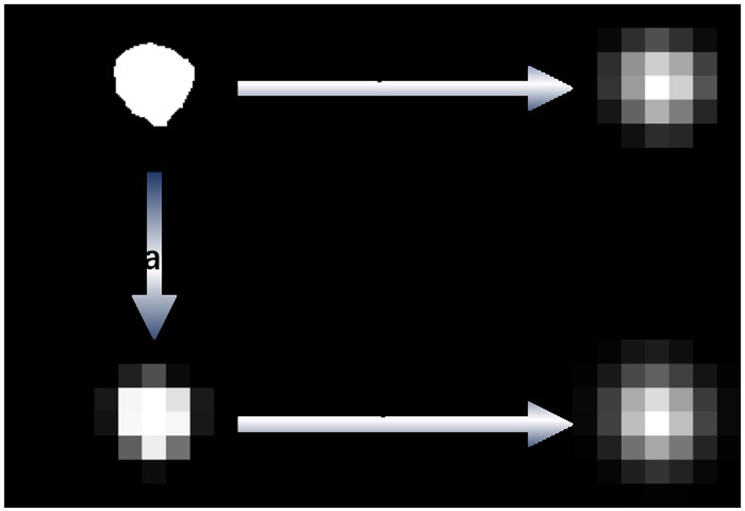
Illustration of different imputation methods of RXD-G and RXD-L, where L-imputation and G-imputation represent the imputation methods of RXD-L and RXD-G, respectively. For RXD-G, original explanation annotations are first down sampled to 7 × 7. Then, the down sampled annotations are imputed by a 3 × 3 Gaussian kernel with Gaussian standard deviation of 0. For RXD-L, original explanation annotations are imputed by a convolution kernel of size 64, stride 32, and padding 16.
Based on that explanation supervision also exploits the rich information in explanation annotations and is thus particularly advantageous when only a few samples are available, we trained our method with sample sizes of 10, 30, 50 and 100. These samples were obtained by a balancing approach: first, half of the samples were drawn from all positive samples in the training set; second, the other half of the samples were drawn from all negative samples in the training set with the same patient IDs as the positive samples. Random horizontal flipping was applied to the samples in training. To accelerate the validation, each time we drew 10% of the positive and negative samples from the validation set. All models were trained using the Adam48 optimizer with a learning rate set to 0.0001 and a batch size of 20. After up to 50 epochs of training, the model with the best AUC in validation was used for testing. Our method was implemented using the deep learning library Pytorch49, based on a graphics processing unit (GPU) NVIDIA T4.
2.4. Performance evaluation
We conducted a comparative study to evaluate the performance of RXD-G and RXD-L. The benchmarks we used included baseline ResNet18, a false positive reduction method called Models Genesis (MG50) and an explanation supervision method called HAICS32. MG is a powerful self-supervised learning framework that uses anatomical structures commonly found in medical images as supervised signals, significantly outperforming scratch learning models50. Its 2D version was used in our comparison. HAICS is a recently proposed framework, which utilizes scribbled annotations as supervision signals32. Its implementation for image classification tasks was used in our comparison. For a fair comparison, all methods used the same backbone DNN (i.e., ResNet18) and were trained with the same settings as in Section 2.3.3.
The classification performance and explanation quality of our RXD-G and RXD-L, baseline (ResNet18), MG and HAICS in terms of reducing false positives are analyzed. The AUC (area under the curve) is used as a measure of classification performance. IoU (Intersection over Union) is used to measure the quality of explanation. This work aims to explore the RXD framework regarding small datasets learning, and we designed numerical experiment using training data with different sample sizes including 10, 30, 50, and 100 samples to evaluate the proposed framework. The framework integrates the deep neural networks and Gaussian and learnable kernels to achieve lung nodule detection with heat maps. These kernel functions with different random seeds results in stochastic outputs from the proposed framework. Based on the previous investigations51,52, five trials with different random seeds can achieve consistent model response while training a deep learning-based model. This work focuses on the feasibility study of using explainable AI to learn from small datasets for accurate pulmonary nodule detection. Therefore, we used the suggested five trials from the previous work51,52 for learning from each dataset with different sample sizes. In each trial, we sampled from the training and validation sets with different random seeds. A case study is also conducted to provide a human assessment of interpretability, where attention maps for all methods trained with sample sizes of 10, 30, 50 and 100 are shown. To further compare the explanation quality of all methods with sample sizes of 50 and 100, the IoUs calculated using different thresholds for the model explanations (since they are continuous) are shown.
3. Results
3.1. Sensitivity analysis of hyper-parameter
The hyper-parameter in Eq. (4) represents the human expected priors of the ideal nodule and non-nodule distributions. Since the actual distributions are usually unknown, the optimal value for varies depending on the dataset and the quality of explanation annotations. Figure 4 depicts the hyper-parameter sensitivity analysis for searching the optimal values based on LIDC-IDRI dataset with different sample sizes. By definition, ranges from 0 to 1. According to the curves in Figure 4, the model AUC and IoU vary with , reaching a peak when equals 0.003 for all sample sizes. The optimal hyper-parameter setting was applied to both RXD-L and RXD-G, since they share the same assumption about ideal nodule and non-nodule distributions.
Figure 4.
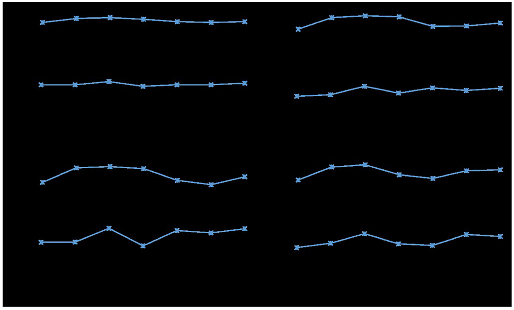
Mean AUC and IoU for different hyper-parameter values of RXD-G with a sample size of (a) 10, (b) 30, (c) 50 and (d) 100 through five trials.
3.2. Quantitative analysis of model performance
The quantitative measurement of classification performance and explanation quality are presented in table 2. In general, our RXD-G and RXD-L outperformed other methods in both classification performance and explanation quality. Specifically, RXD-G beat all other methods in terms of AUC with sample sizes of 10, 30, 50 and 100, and had a higher IoU, showing a robust capacity. For RXD-L, although it did not differ significantly from the baseline in terms of AUC, it still offered a huge improvement in terms of IoU. Specifically, RXD-L improved IoU by 24.0% to 80.0% compared to the baseline. RXD-G achieved even greater improvements, improving by 38.4% to 118.8%.
Table 2.
Performance is compared to Baseline (ResNet18), Models Genesis (MG) and HAICS with sample sizes of 10, 30, 50 and 100. At each sample size, the best results for each metric are in bold, with the second-best results being double underlined. The values in parentheses indicate the percentage improvement compared to the baseline trained with the same sample size. The means and standard deviations are calculated based on five trials with different seeds.
| Sample size | Method | AUC↑ | Enhancement from Baseline | IoU↑ | Enhancement from Baseline |
|---|---|---|---|---|---|
| 10 | Baseline | 0.661±0.023 | - | 0.033±0.009 | - |
| MG | 0.600±0.043 | (−9.3%) | 0.032±0.022 | (−4.5%) | |
| HAICS | 0.669±0.052 | (1.1%) | 0.027±0.015 | (−18.3%) | |
| RXD-L (proposed) | 0.665±0.058 | (0.3%) | 0.042±0.036 | (24.0%) | |
| RXD-G (proposed) | 0.670±0.021 | (1.2%) | 0.046±0.033 | (38.4%) | |
|
| |||||
| 30 | Baseline | 0.709±0.038 | - | 0.029±0.011 | - |
| MG | 0.668±0.046 | (−5.7%) | 0.047±0.008 | (63.2%) | |
| HAICS | 0.710±0.056 | (0.2%) | 0.043±0.004 | (47.6%) | |
| RXD-L (proposed) | 0.698±0.061 | (−1.6%) | 0.050±0.006 | (73.6%) | |
| RXD-G (proposed) | 0.722±0.046 | (1.9%) | 0.063±0.015 | (118.8%) | |
|
| |||||
| 50 | Baseline | 0.753±0.025 | - | 0.039±0.015 | - |
| MG | 0.669±0.060 | (−11.2%) | 0.042±0.009 | (7.8%) | |
| HAICS | 0.751±0.029 | (−0.3%) | 0.056±0.014 | (44.4%) | |
| RXD-L (proposed) | 0.752±0.013 | (−0.2%) | 0.064±0.007 | (66.8%) | |
| RXD-G (proposed) | 0.764±0.038 | (1.4%) | 0.069±0.010 | (80.0%) | |
|
| |||||
| 100 | Baseline | 0.834±0.018 | - | 0.050±0.006 | - |
| MG | 0.735±0.040 | (−11.9%) | 0.059±0.006 | (19.6%) | |
| HAICS | 0.820±0.014 | (−1.7%) | 0.092±0.019 | (86.7%) | |
| RXD-L (proposed) | 0.831±0.016 | (−0.4%) | 0.089±0.013 | (79.8%) | |
| RXD-G (proposed) | 0.836±0.014 | (0.2%) | 0.086±0.007 | (73.9%) | |
This suggests that for pulmonary nodules, the Gaussian imputation method works better on small sample sizes. This makes sense because a single-layer imputation block may not be capable of learning such a variety of nodule morphologies, while a pre-defined Gaussian kernel can be less affected.
To show the improvement in training sample utilization efficiency, we report the decrease in AUC of RXD-G compared to baseline. Figure 5 shows the percentage decrease in AUC of baseline and RXD-G trained with smaller sample sizes compared to the AUC of baseline trained on 100 samples. At each sample size, the longer the bar, the more AUC decreases from baseline trained on 100 samples. In all cases, the decrease in AUC of RXD-G is smaller than baseline, indicating that RXD improves the utilization efficiency of the training samples.
Figure 5.
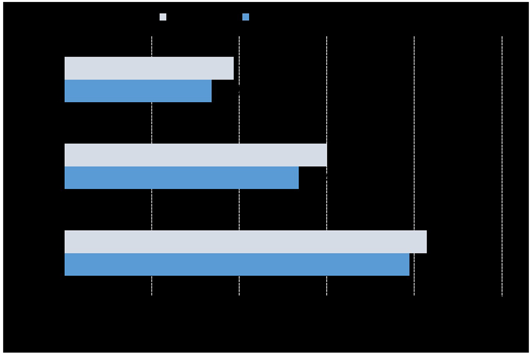
Percentage decrease in AUC of baseline and RXD-G trained on smaller sample sizes compared to the AUC of baseline trained on 100 samples through five trials. The gray and blue bars represent the decrease in AUC for baseline and RXD-G, respectively. At each sample size, the longer the bar, the more the AUC decreases compared to the AUC of the baseline trained on 100 samples.
3.3. Qualitative analysis of explanation quality
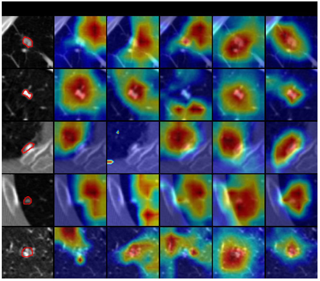
A case study is conducted to compare the explanation quality of all models. Model-generated explanations are presented by overlaying a heatmap on the original image, where the warmer colored regions are given more importance. Figures 6–9 show some explanation visualization results of all models with sample sizes of 10, 30, 50 and 100, respectively. The first column is the original image, where nodule region is circled in red. The following columns are model explanations generated by baseline, MG (i.e., Models Genesis), HAICS, RXD-L and RXD-G, respectively. Ideally, the warm regions in model explanation should overlap precisely with the nodule regions in each row, indicating that the prediction is completely dependent on the nodule regions. In general, all models yielded more consistent explanations with the nodule regions when trained on a larger sample size. Baseline was more concentrated in non-nodule areas, showing a serious bias. MG can focus on the right area, but with severe imprecision. HAICS produced precise attributions but can be severely biased if trained on insufficient samples. RXD-L and RXD-G can correctly focus on the nodule region even when trained on a small number of samples, with RXD-L performing less biased and RXD-G more precise.
Figure 6.
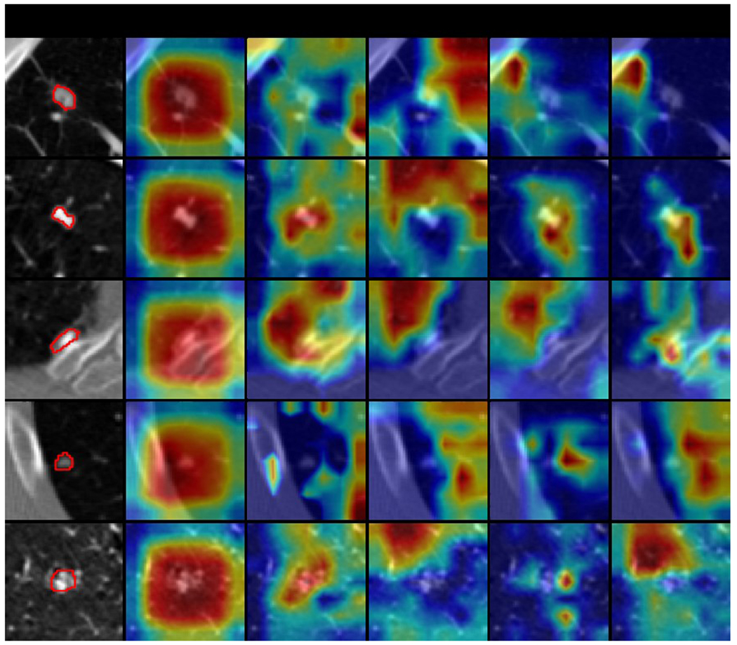
Selected explanation visualization results of all methods with sample size of 10. In the first column, the ground truth nodule region is circled in red. The model-generated explanations are represented by heatmaps overlaid on the original images, where the warmer colored regions are given more importance. Baseline refers to ResNet18, MG and HAICS are comparative methods, while RXD-G and RXD-L are our methods.
Figure 9.
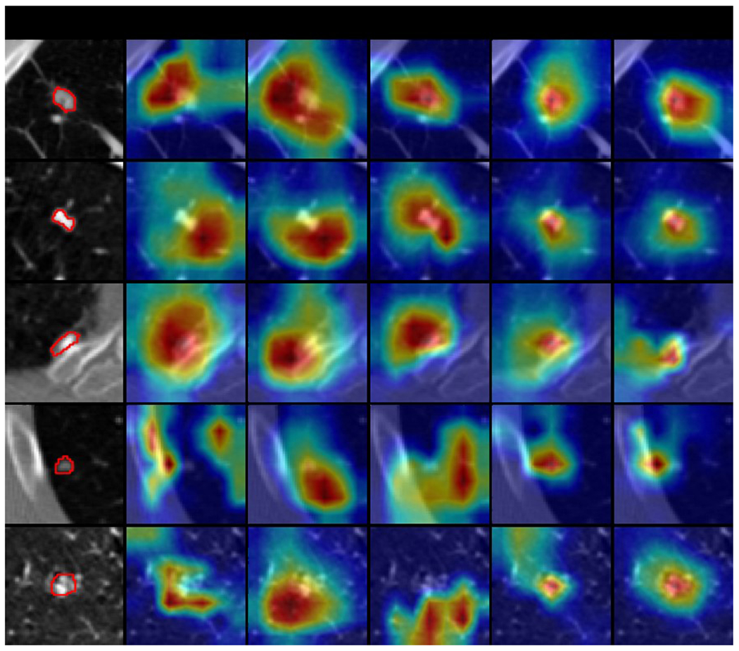
Selected explanation visualization results of all methods with sample size of 100. In the first column, the ground truth nodule region is circled in red. The model-generated explanations are represented by heatmaps overlaid on the original images, where the warmer colored regions are given more importance. Baseline refers to ResNet18, MG and HAICS are comparative methods, while RXD-G and RXD-L are our methods.
3.4. Quantitative analysis of explanation quality
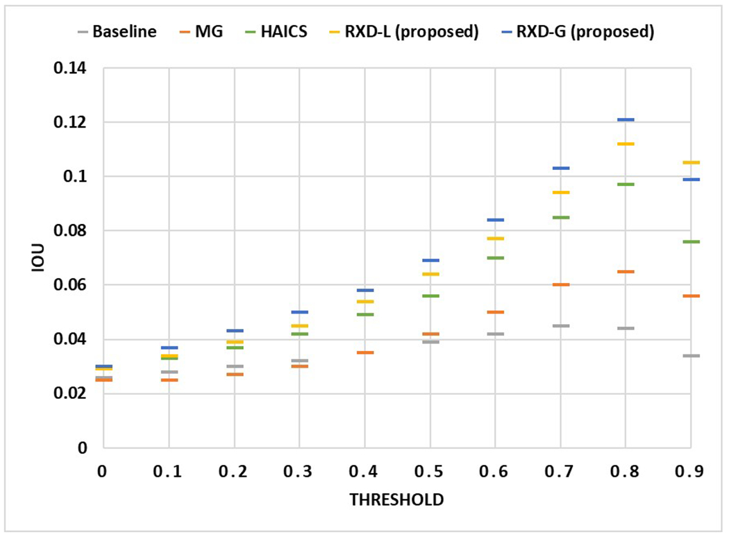
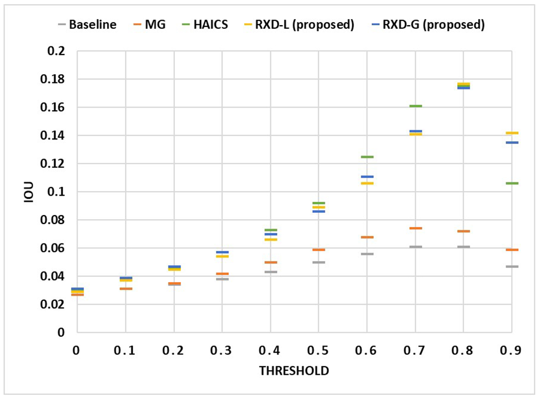
The previous experiment shows the model explanations for only a few samples. For a more comprehensive study, we changed the threshold of attention values in model explanations and recomputed IoU. When the threshold is small (e.g., 0.1), regions with very low influence on the model prediction results are also used to compute the degree of overlap with the nodule region; when the threshold is high (e.g., 0.9), only regions with high influence on the model prediction results are used to compute the degree of overlap with the nodule region. Using Figure 9 to better illustrate, the yellow-green areas in the model explanation may have an attention value of 0.1, while the red areas in the model explanation may have an attention value of 0.9. Figures 10 and 11 show the IoU obtained by each model using different thresholds of attention values when the sample size is 50 and 100, respectively, with the horizontal axis showing the different attention value thresholds and the vertical axis showing the average IoU, and all data points are the average of the model test results obtained through five trials. In general, the highest IoU is obtained for all models when the threshold is around 0.8. When the sample size is 50, RXD-G and RXD-L obtained the highest and second highest results at each threshold, respectively, with HAICS in third place, while Models Genesis and Baseline were significantly lagged. This contrast is more pronounced when the sample size is 100 and the gap between HAICS and RXD-L and RXD-G became smaller. Regardless of the sample size, the IoU of Models Genesis and baseline is low at every threshold, suggesting that neither relies primarily on the nodule region for classification. In contrast, explanation supervision methods (HAICS, RXD-L and RXD-G) are highly dependent on nodule regions, suggesting that explanation supervision methods are able to learn attributions that are more consistent with human cognition.
Figure 10.
The IoU obtained by each method using different attention value thresholds when the sample size is 50. The horizontal axis shows the different attention value thresholds, and the vertical axis shows the average IoU. All data points are the average of the model test results obtained through five trials.
Figure 11.
The IoU obtained by each method using different attention value thresholds when the sample size is 100. The horizontal axis shows the different attention value thresholds, and the vertical axis shows the average IoU. All data points are the average of the model test results obtained through five trials.
4. Discussion
Pulmonary nodule detection is essential for early diagnosis of potential lung cancer, which can significantly improve the survival rate. Since not all nodules are cancerous, it is critical for a computer algorithm to track the geometrical feature of nodules such that radiologists can evaluate if a nodule is growing over time. Training on images without any guidance will cause the model to focus on meaningless regions. Whereas humans, especially experts, focus their attention on important parts with key information (e.g., module regions), which would be more effective. Aligning the model's focus with that of humans through an explanation-guided training process prevents sub-optimal models from wasting attention on trivial regions. With a robust learning framework, the model is able to filter annotation noise, resulting in better performance. The proposed pulmonary nodule detection framework delivers both classification results to indicate the presence of nodules and heat maps to present the likelihood of how DL models learn nodule distribution based on patient anatomy. Such a framework can help us understand if the DL model predicts the results by coincidence or if the model learns the spatial distribution of pulmonary nodules, which is helpful for lung lesion prognosis.
Table 2 indicates that the baseline consistently achieves stable classification performance with an average AUC of 0.74±0.07 regarding different training sample sizes. However, its average IoU is 0.04±0.01, which indicates that the baseline does not learn much of the nodule morphology. This model has limited values as it cannot provide spatial details of nodules to allow radiologists to further investigate the risk of potentially cancerous lesions. For small dataset learning (sample size=30), the proposed RXD-G can enhance the AUC and IoU values by 1.9% and 118.8%, compared to the baseline. Even in the extreme case (sample size=10), RXD-G can still increase the AUC and IoU values by 1.2% and 38.4% from the baseline model. Figure 5 shows that the AUC of RXD-G drops by 13.4% when the training sample size decreases from 100 to 50. In contrast, the AUC of the baseline reduces by 15%. These observations suggest that the proposed framework achieves the optimal nodule classification performance and explanation quality for small dataset learning, including sample sizes from 10 to 50.
Interpretability is another important aspect to assess an explainable AI. In this sense, beyond the calculation of IoU in a single case, a more comprehensive comparison is needed. Figures 6–9 exhibit model explanations in real scenarios where the model explanations are overlaid on the original images in the form of heatmaps. Nodule regions are relatively small and provide a difficult attribution test for all methods. The baseline and the two comparative methods expose their poor attribution, with either high bias or high variance. While our RXD-L and RXD-G constantly focus on the nodule region, with RXD-L less biased and RXD-G more precise. The color indicates the importance for the prediction. A model can assign high importance to incorrect regions, or low importance to correct regions. To evaluate model attributions in all cases, we change the threshold of attention values and recompute IoU. Figure 10 and Figure 11 show the IoU curves with different thresholds, where there is a clear distinction between explanation supervision methods and others. In particular, when sample size is small (sample size=50), our RXD-L and RXD-G have better consistency between model attributions and expert attributions.
DNN with multilayer perceptrons has been proven to be a universal approximator53, and its hierarchical model structures can determine the underlying non-linear correlation behind the data54,55. However, the selection of hyper-parameters can impact the learning performance of DNN. Figure 4 shows the sensitivity analysis for the hyper-parameter , which regularizes the explanation loss given in Eq. (4). Since the goal is to achieve optimal nodule classification and morphology results, the should be 0.003 in this work to maximize the AUC and IoU values. The proposed framework can achieve optimal AUC and IoU values when the training samples are less than 50. The generated heatmaps indicate the importance of weighting for nodule regions on the CT images. Future work will likely focus on providing the probability distribution maps of lung nodules to support the diagnosis and prognosis of cancerous lung nodules and risk-informed medical decision-making.
5. Conclusions
A pulmonary nodule detection framework was demonstrated with expandability using the nonproprietary LIDC-IDRI dataset. The proposed framework enables the DL models to learn nodule classification, and most importantly, the proposed method ensures that the models consistently forecast nodule morphology as expected from human perspectives. The method can enhance the accuracy of computer-aided nodule detection systems and reduce the uncertainty of misclassification due to human factors. Such a method can reduce the workload of radiologists and enable them to focus on investigating the prognosis of cancerous nodules for early treatment to improve patient outcomes and survival rates.
Figure 7.
Selected explanation visualization results of all methods with sample size of 30. In the first column, the ground truth nodule region is circled in red. The model-generated explanations are represented by heatmaps overlaid on the original images, where the warmer colored regions are given more importance. Baseline refers to ResNet18, MG and HAICS are comparative methods, while RXD-G and RXD-L are our methods.
Figure 8.
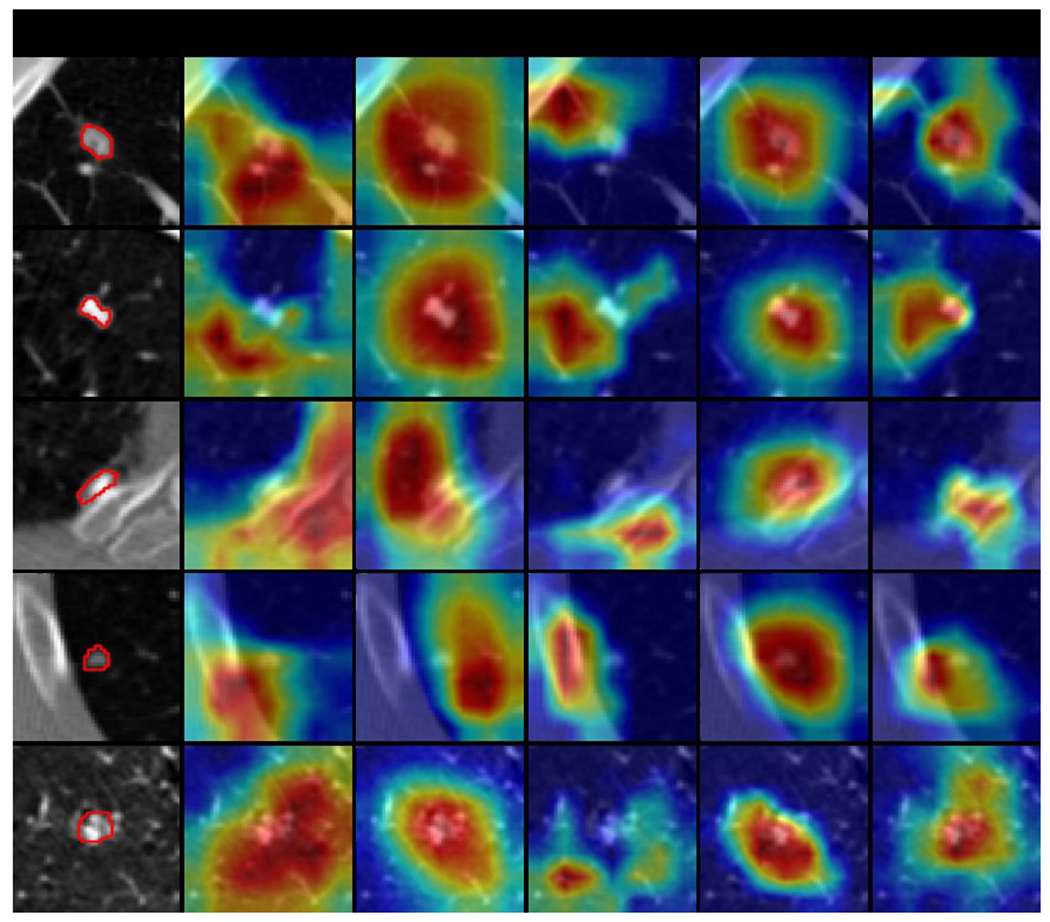
Selected explanation visualization results of all methods with sample size of 50. In the first column, the ground truth nodule region is circled in red. The model-generated explanations are represented by heatmaps overlaid on the original images, where the warmer colored regions are given more importance. Baseline refers to ResNet18, MG and HAICS are comparative methods, while RXD-G and RXD-L are our methods.
Acknowledgments
This work is supported by the National Institutes of Health under Award Number R01CA215718, R01CA272991, R56EB033332 and R01EB032680, the NSF Grant No. 2007716, No. 2007976, No. 1942594, No. 1907805, No. 1841520 and No. 1755850, Meta Research Award, NEC Lab, Amazon Research Award, Oracle for Research Grant Award, Cisco Faculty Research Award, COMPUTING RESEARCH ASSOCIATION / NSF Sub: 2021CIF-Emory-05. Also, the Department of Homeland Security (DHS) has supported this work via the grant with Grant No. 17STCIN00001. The authors acknowledge the National Cancer Institute and the Foundation for the National Institutes of Health, and their critical role in the creation of the free publicly available LIDC/IDRI Database used in this study.
Footnotes
Conflict of interest
The authors have no conflict of interests to disclose.
Ethical Statement
All patient CT images were acquired from the public database, Lung Image Database Consortium and Image Database Resource Initiative (LIDC-IDRI) dataset.
References
- 1.Investigators IELCAP. Survival of patients with stage I lung cancer detected on CT screening. New England Journal of Medicine. 2006;355(17):1763–1771. [DOI] [PubMed] [Google Scholar]
- 2.Diederich S, Das M. Solitary pulmonary nodule: detection and management. Cancer Imaging. 2006;6(Spec No A):S42. [DOI] [PMC free article] [PubMed] [Google Scholar]
- 3.Chen H, Huang S, Zeng Q, et al. A retrospective study analyzing missed diagnosis of lung metastases at their early stages on computed tomography. J Thorac Dis. 2019;11(8):3360–3368. [DOI] [PMC free article] [PubMed] [Google Scholar]
- 4.Way TW, Hadjiiski LM, Sahiner B, et al. Computer-aided diagnosis of pulmonary nodules on CT scans: Segmentation and classification using 3D active contours. Medical Physics. 2006;33(7Part1):2323–2337. [DOI] [PMC free article] [PubMed] [Google Scholar]
- 5.Hu M, Wang J, Chang C-W, Liu T, Yang X. End-to-end brain tumor detection using a graph-feature-based classifier. Vol 12468: SPIE; 2023. [Google Scholar]
- 6.Yang Y, Li X, Fu J, Han Z, Gao B. 3D multi-view squeeze-and-excitation convolutional neural network for lung nodule classification. Medical Physics. 2023;50(3):1905–1916. [DOI] [PubMed] [Google Scholar]
- 7.Liu L, Wolterink JM, Brune C, Veldhuis RNJ. Anatomy-aided deep learning for medical image segmentation: a review. Physics in Medicine & Biology. 2021;66(11):11TR01. [DOI] [PubMed] [Google Scholar]
- 8.Pan S, Chang C-W, Wang T, et al. Abdomen CT multi-organ segmentation using token-based MLP-Mixer. Medical Physics. 2022;n/a(n/a). [DOI] [PMC free article] [PubMed] [Google Scholar]
- 9.Zhang F, Wang Q, Fan E, et al. Automatic segmentation of the tumor in nonsmall-cell lung cancer by combining coarse and fine segmentation. Medical Physics. 2023;50(6):3549–3559. [DOI] [PubMed] [Google Scholar]
- 10.Chen H, Gomez C, Huang C-M, Unberath M. Explainable medical imaging AI needs human-centered design: guidelines and evidence from a systematic review. npj Digital Medicine. 2022;5(1):156. [DOI] [PMC free article] [PubMed] [Google Scholar]
- 11.Fuhrman JD, Gorre N, Hu Q, Li H, El Naqa I, Giger ML. A review of explainable and interpretable AI with applications in COVID-19 imaging. Medical Physics. 2022;49(1):1–14. [DOI] [PMC free article] [PubMed] [Google Scholar]
- 12.Ronneberger O, Fischer P, Brox T. U-net: Convolutional networks for biomedical image segmentation. Paper presented at: Medical Image Computing and Computer-Assisted Intervention–MICCAI 2015: 18th International Conference, Munich, Germany, October 5–9, 2015, Proceedings, Part III 18; 2015, 2015. [Google Scholar]
- 13.Christ PF, Elshaer MEA, Ettlinger F, et al. Automatic liver and lesion segmentation in CT using cascaded fully convolutional neural networks and 3D conditional random fields. Paper presented at: International conference on medical image computing and computer-assisted intervention; 2016, 2016. [Google Scholar]
- 14.Wang G, Li W, Ourselin S, Vercauteren T. Automatic brain tumor segmentation using convolutional neural networks with test-time augmentation. Paper presented at: Brainlesion: Glioma, Multiple Sclerosis, Stroke and Traumatic Brain Injuries: 4th International Workshop, BrainLes 2018, Held in Conjunction with MICCAI 2018, Granada, Spain, September 16, 2018, Revised Selected Papers, Part II 4; 2019, 2019. [Google Scholar]
- 15.Wu W, Gao L, Duan H, Huang G, Ye X, Nie S. Segmentation of pulmonary nodules in CT images based on 3D-UNET combined with three-dimensional conditional random field optimization. Medical Physics. 2020;47(9):4054–4063. [DOI] [PubMed] [Google Scholar]
- 16.Chen H, Dou Q, Yu L, Qin J, Heng P-A. VoxResNet: Deep voxelwise residual networks for brain segmentation from 3D MR images. NeuroImage. 2018;170:446–455. [DOI] [PubMed] [Google Scholar]
- 17.Huff DT, Weisman AJ, Jeraj R. Interpretation and visualization techniques for deep learning models in medical imaging. Physics in Medicine & Biology. 2021;66(4):04TR01. [DOI] [PMC free article] [PubMed] [Google Scholar]
- 18.Jin H, Li Z, Tong R, Lin L. A deep 3D residual CNN for false-positive reduction in pulmonary nodule detection. Medical physics. 2018;45(5):2097–2107. [DOI] [PubMed] [Google Scholar]
- 19.Winkels M, Cohen TS. Pulmonary nodule detection in CT scans with equivariant CNNs. Medical image analysis. 2019;55:15–26. [DOI] [PubMed] [Google Scholar]
- 20.Wu Z, Ge R, Shi G, et al. MD-NDNet: a multi-dimensional convolutional neural network for false-positive reduction in pulmonary nodule detection. Physics in Medicine & Biology. 2020;65(23):235053. [DOI] [PubMed] [Google Scholar]
- 21.Mei J, Cheng M-M, Xu G, Wan L-R, Zhang H. SANet: A slice-aware network for pulmonary nodule detection. IEEE transactions on pattern analysis and machine intelligence. 2021;44(8):4374–4387. [DOI] [PubMed] [Google Scholar]
- 22.Bach S, Binder A, Montavon G, Klauschen F, Müller K-R, Samek W. On pixel-wise explanations for non-linear classifier decisions by layer-wise relevance propagation. PloS one. 2015;10(7):e0130140. [DOI] [PMC free article] [PubMed] [Google Scholar]
- 23.Bojarski M, Choromanska A, Choromanski K, et al. Visualbackprop: visualizing cnns for autonomous driving. arXiv preprint arXiv:161105418. 2016;2. [Google Scholar]
- 24.Montavon G, Lapuschkin S, Binder A, Samek W, Müller K-R. Explaining nonlinear classification decisions with deep taylor decomposition. Pattern Recognition. 2017;65:211–222. [Google Scholar]
- 25.Montavon G, Binder A, Lapuschkin S, Samek W, Müller K-R. Layer-wise relevance propagation: an overview. Explainable AI: interpreting, explaining and visualizing deep learning. 2019.193–209. [Google Scholar]
- 26.Zhou B, Khosla A, Lapedriza A, Oliva A, Torralba A. Learning deep features for discriminative localization. Paper presented at: Proceedings of the IEEE conference on computer vision and pattern recognition; 2016, 2016. [Google Scholar]
- 27.Selvaraju RR, Cogswell M, Das A, Vedantam R, Parikh D, Batra D. Grad-cam: Visual explanations from deep networks via gradient-based localization. Paper presented at: Proceedings of the IEEE international conference on computer vision; 2017, 2017. [Google Scholar]
- 28.Gao Y, Gu S, Jiang J, Hong SR, Yu D, Zhao L. Going Beyond XAI: A Systematic Survey for Explanation-Guided Learning. arXiv preprint arXiv:221203954. 2022. [Google Scholar]
- 29.Linsley D, Shiebler D, Eberhardt S, Serre T. Learning what and where to attend. arXiv preprint arXiv:180508819. 2018. [Google Scholar]
- 30.Mitsuhara M, Fukui H, Sakashita Y, et al. Embedding human knowledge into deep neural network via attention map. arXiv preprint arXiv:190503540. 2019. [Google Scholar]
- 31.Fukui H, Hirakawa T, Yamashita T, Fujiyoshi H. Attention branch network: Learning of attention mechanism for visual explanation. Paper presented at: Proceedings of the IEEE/CVF conference on computer vision and pattern recognition; 2019, 2019. [Google Scholar]
- 32.Shen H, Liao K, Liao Z, et al. Human-AI interactive and continuous sensemaking: A case study of image classification using scribble attention maps. Paper presented at: Extended Abstracts of the 2021 CHI Conference on Human Factors in Computing Systems; 2021, 2021. [Google Scholar]
- 33.Gao Y, Sun TS, Zhao L, Hong SR. Aligning eyes between humans and deep neural network through interactive attention alignment. Proceedings of the ACM on Human-Computer Interaction. 2022;6(CSCW2):1–28.37360538 [Google Scholar]
- 34.Gao Y, Sun TS, Bai G, Gu S, Hong SR, Liang Z. RES: A Robust Framework for Guiding Visual Explanation. Paper presented at: Proceedings of the 28th ACM SIGKDD Conference on Knowledge Discovery and Data Mining; 2022, 2022. [Google Scholar]
- 35.Chang C-W, Gao Y, Wang T, et al. Dual-energy CT based mass density and relative stopping power estimation for proton therapy using physics-informed deep learning. Physics in Medicine & Biology. 2022;67(11):115010. [DOI] [PMC free article] [PubMed] [Google Scholar]
- 36.Chang C-W, Zhou S, Gao Y, et al. Validation of a deep learning-based material estimation model for Monte Carlo dose calculation in proton therapy. Physics in Medicine & Biology. 2022;67(21):215004. [DOI] [PMC free article] [PubMed] [Google Scholar]
- 37.Armato Iii SG, McLennan G, Bidaut L, et al. The Lung Image Database Consortium (LIDC) and Image Database Resource Initiative (IDRI): A Completed Reference Database of Lung Nodules on CT Scans. Medical Physics. 2011;38(2):915–931. [DOI] [PMC free article] [PubMed] [Google Scholar]
- 38.Clark K, Vendt B, Smith K, et al. The Cancer Imaging Archive (TCIA): Maintaining and Operating a Public Information Repository. Journal of Digital Imaging. 2013;26(6):1045–1057. [DOI] [PMC free article] [PubMed] [Google Scholar]
- 39.Armato SG III, McLennan G, Bidaut L, McNitt-Gray MF, Meyer CR, Reeves AP, Zhao B, Aberle DR, Henschke CI, Hoffman EA, Kazerooni EA, MacMahon H, Van Beek EJR, Yankelevitz D, Biancardi AM, Bland PH, Brown MS, Engelmann RM, Laderach GE, Max D, Pais RC, Qing DPY, Roberts RY, Smith AR, Starkey A, Batra P, Caligiuri P, Farooqi A, Gladish GW, Jude CM, Munden RF, Petkovska I, Quint LE, Schwartz LH, Sundaram B, Dodd LE, Fenimore C, Gur D, Petrick N, Freymann J, Kirby J, Hughes B, Casteele AV, Gupte S, Sallam M, Heath MD, Kuhn MH, Dharaiya E, Burns R, Fryd DS, Salganicoff M, Anand V, Shreter U, Vastagh S, Croft BY, Clarke LP. Data From LIDC-IDRI The Cancer Imaging Archive. 2015. doi: 10.7937/K9/TCIA.2015.LO9QL9SX. [DOI] [Google Scholar]
- 40.Bv Ginneken, Setio AAA, Jacobs C, Ciompi F. Off-the-shelf convolutional neural network features for pulmonary nodule detection in computed tomography scans. Paper presented at: 2015 IEEE 12th International Symposium on Biomedical Imaging (ISBI); 16-19 April 2015, 2015. [Google Scholar]
- 41.Zhang G, Jiang S, Yang Z, et al. Automatic nodule detection for lung cancer in CT images: A review. Computers in Biology and Medicine. 2018;103:287–300. [DOI] [PubMed] [Google Scholar]
- 42.Zhou Z, Rahman Siddiquee MM, Tajbakhsh N, Liang J. Unet++: A nested u-net architecture for medical image segmentation. Paper presented at: Deep Learning in Medical Image Analysis and Multimodal Learning for Clinical Decision Support: 4th International Workshop, DLMIA 2018, and 8th International Workshop, ML-CDS 2018, Held in Conjunction with MICCAI 2018, Granada, Spain, September 20, 2018, Proceedings 4; 2018, 2018. [DOI] [PMC free article] [PubMed] [Google Scholar]
- 43.Armato SG III, McLennan G, McNitt-Gray MF, et al. Lung image database consortium: developing a resource for the medical imaging research community. Radiology. 2004;232(3):739–748. [DOI] [PubMed] [Google Scholar]
- 44.Armato Iii SG, McLennan G, Bidaut L, et al. The lung image database consortium (LIDC) and image database resource initiative (IDRI): a completed reference database of lung nodules on CT scans. Medical physics. 2011;38(2):915–931. [DOI] [PMC free article] [PubMed] [Google Scholar]
- 45.McNitt-Gray MF, Armato SG III, Meyer CR, et al. The Lung Image Database Consortium (LIDC) data collection process for nodule detection and annotation. Academic radiology. 2007;14(12):1464–1474. [DOI] [PMC free article] [PubMed] [Google Scholar]
- 46.Hancock MC, Magnan JF. Lung nodule malignancy classification using only radiologist-quantified image features as inputs to statistical learning algorithms: probing the Lung Image Database Consortium dataset with two statistical learning methods. Journal of Medical Imaging. 2016;3(4):044504–044504. [DOI] [PMC free article] [PubMed] [Google Scholar]
- 47.He K, Zhang X, Ren S, Sun J. Deep residual learning for image recognition. Paper presented at: Proceedings of the IEEE conference on computer vision and pattern recognition; 2016, 2016. [Google Scholar]
- 48.Kingma DP, Ba J. Adam: A method for stochastic optimization. arXiv preprint arXiv:14126980. 2014. [Google Scholar]
- 49.Paszke A, Gross S, Massa F, et al. Pytorch: An imperative style, high-performance deep learning library. Advances in neural information processing systems. 2019;32. [Google Scholar]
- 50.Zhou Z, Sodha V, Rahman Siddiquee MM, et al. Models genesis: Generic autodidactic models for 3d medical image analysis. Paper presented at: Medical Image Computing and Computer Assisted Intervention–MICCAI 2019: 22nd International Conference, Shenzhen, China, October 13–17, 2019, Proceedings, Part IV 22; 2019, 2019. [DOI] [PMC free article] [PubMed] [Google Scholar]
- 51.Paing MP, Hamamoto K, Tungjitkusolmun S, Pintavirooj C. Automatic detection and staging of lung tumors using locational features and double-staged classifications. Applied Sciences. 2019;9(11):2329. [Google Scholar]
- 52.Kadry S, Rajinikanth V, Rho S, Raja NSM, Rao VS, Thanaraj KP. Development of a machine-learning system to classify lung CT scan images into normal/COVID-19 class. arXiv preprint arXiv:200413122. 2020. [Google Scholar]
- 53.Hornik K, Stinchcombe M, White H. Multilayer feedforward networks are universal approximators. Neural Networks. 1989;2(5):359–366. [Google Scholar]
- 54.LeCun Y, Bengio Y, Hinton G. Deep learning. Nature. 2015;521(7553):436–444. [DOI] [PubMed] [Google Scholar]
- 55.Chang C-W, Dinh NT. Classification of machine learning frameworks for data-driven thermal fluid models. International Journal of Thermal Sciences. 2019;135:559–579. [Google Scholar]