Behavioral game of quarantine during the monkeypox epidemic: Analysis of deterministic and fractional order approach

Abstract

This work concerns the epidemiology of infectious diseases like monkeypox (mpox) in humans and animals. Our models examine transmission scenarios, including transmission dynamics between humans, animals, and both. We approach this using evolutionary game theory, specifically the intervention game-theoretical (IGT) framework, to study how human behavior can mitigate disease transmission without perfect vaccines and treatments. To do this, we use non-pharmaceutical intervention, namely the quarantine policy, which demonstrates the delayed effect of the epidemic. Additionally, we contemplate quarantine-based behavioral intervention policies in deterministic and fractional-order models to show behavioral impact in the context of the memory effect. Firstly, we extensively analyzed the model's positivity and boundness of the solution, reproduction number, disease-free and endemic equilibrium, possible stability, existence, concavity, and Ulam-Hyers stability for the fractional order. Subsequently, we proceeded to present a numerical analysis that effectively illustrates the repercussions of varying quarantine-related factors, information probability, and protection probability. We aimed to comprehensively examine the effects of non-pharmaceutical interventions on disease control, which we conveyed through line graphs and 2D heat maps. Our findings underscored the significant influence of strict quarantine measures and the protection of both humans and animals in mitigating disease outbreaks. These measures not only significantly curtailed the spread of the disease but also delayed the occurrence of the epidemic's peak. Conversely, when quarantine maintenance policies were implemented at lower rates and protection levels diminished, we observed contrasting outcomes that exacerbated the situation. Eventually, our analysis revealed the emergence of animal reservoirs in cases involving disease transmission between humans and animals.

1. Introduction

The monkeypox virus (mpoxv), which causes monkeypox (mpox), is a zoonotic disease mainly transferred from animals to humans. It was first identified in 1958 after two disease outbreaks mimicking the mpox in groups of monkeys [1]. Moreover, mpox virus infection has been detected in squirrels, rats obtained from Gambian slums, dormice, several monkey species, and other animals [2]. Mpox disease is transferred among individuals in human society by direct contact with an infectious rash, scabs, or bodily fluids. The exchange of respiratory secretions during extended face-to-face contact, sexual activity, or close physical touch is the second mechanism of transmission [[3], [4], [5], [6]]. Thirdly, the World Health Organization (WHO) declared that mpox disease is transferrable from the environment to humans, such as when an infected person touches items such as clothes, bedding, towels, devices, and surfaces. If the person handling the object has wounds or abrasions or inadvertent contact with their eyes, nose, mouth, or other mucous membranes, they risk contracting an infection. In recapitulation, the World Health Organization (WHO) also warns about the potential transmission of the monkeypox virus from people to vulnerable animal species in different settings, which may lead to the development of new animal reservoirs since several animal species are known to be susceptible to the monkeypox virus. Consequently, those diagnosed with or suspect mpox should avoid close physical contact with wild animals and household pets, namely cats, dogs, hamsters, and gerbils [2]. Recently, WHO has received mpox outbreak reports from numerous nations since January 2022, with 2103 cases with laboratory confirmation and one death as of June 15, 2022 [1,2]. After that, policymakers and researchers worldwide rethought the mpox disease. Although some countries are recommending and approving smallpox (MVA-BN and LC16) vaccination (smallpox vaccines have been protective against mpox in the past) for people at risk for mpox prevention, until now, mpox disease has had no proper vaccine or treatment [2]. Considering the above facts, we considered a quarantine-based mathematical epidemic model with and without the probability of transmitting humans to animals (see Table 1).

Table 1.

List of parameters, variables, and their meanings.

Notation	Meaning	Values	Reference
${\mathrm{\Lambda }}_h$	Human growth rate	0.0	Assumed
${\mathrm{\Lambda }}_a$	Animal growth rate	0.0	Assumed
${\beta }_{hh}$	Human to human-transmission rate	1.0	[48]
${\beta }_{aa}$	Animal-to-animal transmission rate	0.5	Assumed
${\phi }_a$	Protection rate against infected animals	0.0, 0.5, 0.9	Assumed
${\phi }_h$	Protection rate against infected humans	0.0, 0.5, 0.9	Assumed
${\alpha }_h$	Humans incubation period	$\left(\frac{1}{5}-\frac{1}{21}\right)$ (days)	[2]
${\alpha }_a$	Animals incubation period	0.2	Assumed
$\delta$	Quarantine or self-isolation period	$\left(\frac{1}{14}-\frac{1}{28}\right)$ (days)	[2]
${\gamma }_h$	Humans recover rate	0.1	[48]
${\gamma }_a$	Animals recover rate	0.1	Assumed
$\theta$	Transmission rate of human to animal	0.0–1.0	Assumed
${\mu }_a$	Natural death rate of infected animals	0.0	Assumed
${\mu }_h$	Natural death rate of infected humans	0.0	Assumed
$C_i$	Infection cost for individuals	1.0	[41,42]
$C_q$	Self-quarantine cost for individuals	0.1, 0.9	Assumed
$\rho$	Information probability of the infected animal	0.1, 0.9	Assumed
$S_h\left(t\right)$	Number of susceptible individuals	0.9999	[54,64,65]
$E_h\left(t\right)$	Number of exposed individuals	0.0	[54,64,65]
$I_h\left(t\right)$	Number of infected individuals	0.0001	[54,64,65]
$Q_h\left(t\right)$	Number of quarantine or self-isolated individuals	0.0	[54,64,65]
$R_h\left(t\right)$	Number of recovered individuals	0.0	[54,64,65]
$S_a\left(t\right)$	Number of susceptible animals	0.9999	Assumed
$E_a\left(t\right)$	Number of exposed animals	0.0	Assumed
$I_a\left(t\right)$	Number of infected animals	0.0001	Assumed
$R_a\left(t\right)$	Number of recovered animals	0.0	Assumed

The mpox disease has mainly been neglected in the past, making the comprehension of its transmission mechanisms challenging. Nevertheless, several scientists have attempted to characterize the dynamics of the mpox virus quantitatively. Peter et al. [7] developed a deterministic mathematical model for the mpox virus, demonstrating that isolating infected individuals from the general community reduces disease transmission. Bhunu and Mushayabasa [8] developed a kinetic model of mpox transmission. Multifaceted mathematical models have been explored to comprehend the improved disease transmission dynamics and the various strategies for controlling the endemic disease (see Refs. [[7], [9], [10], [11], [12], [13], [14], [15]] for more information). According to Bankuru et al. [16] suggested that mpox is manageable and might potentially be eliminated with vaccination in a semi-endemic equilibrium. However, vaccination alone cannot eradicate mpox in a wholly endemic equilibrium. Numerical simulations of the model [17] demonstrate that the proposed activities eradicated infected individuals in both human and monkey populations throughout the research period. Riaz [18] and Focosi et al. [19] extensively examine mpox, including its outbreak and medical appearance, epidemiology, pathological progression, vaccines, and treatments for the human mpox virus. Ola [20] presented that, in contrast to the spread of the monkeypox virus, spectral disorders show symptoms like monkeypox. Maruotti et al. [21] predicted the undetected infection size during the mpox outbreak. Damon [22] describes insights into the mpox virus and its emergence in human populations. Islam et al. [23] argue that the mpox virus does not require terror and stigma; only knowledge and preventative efforts may stop the pandemic turn of this epidemic disease. Peter et al. [7,24] and Qurashi et al. [25] contend that isolating individuals with diseases within the human population is beneficial in reducing disease transmission. They also assert that implementing preventive measures to stop the transmission of diseases from rodents to humans is the most economically efficient approach compared to other alternatives. Therefore, to evaluate the mpox disease incidence and its non-pharmaceutical intervention, we proposed a deterministic method, a fractional order derivative approach including EGT. This combined approach offers a more comprehensive view of the consequences of non-pharmaceutical tactics on the spread of mpox disease. The fractional order derivative approach models the dynamics of the disease, while the EGT considers the behavior of individuals and how they respond to the disease and interventions.

Integrating over a given area makes it possible to obtain a fractional-order derivative. This approach differs from traditional integer-order derivatives in that it accounts for non-local behavior and considers the fractional-order transformations at each instant. Several studies have used fractional-order derivatives to foretell the pandemic's potential outcomes and dynamic aspects [[26], [27], [28], [29], [30], [31], [32], [33]]. The fractional-order epidemic model [[27], [28], [29],34,35] was investigated by many researchers on complex epidemic dynamics, who applied it to topics like different types of epidemic control, the ABO blood group, non-linear incidence rates, and real-world data. Recently, Okyere and Ackora-Prah [36] offered ABC fractional-order derivatives to examine the dynamics of mpox transmission in Ghana. As Peter et al. [37] indicated, a decrease in the order of fractional derivatives is thought to underlie the observed changes. Alharbi et al. [38] investigated the fractional-calculus modeling and stability study of the dynamics of mpox. This research intends to examine the dissemination of mpox disease and the implementation of control measures using conventional and fractional-order models. The objective is to comprehend the memory index's impact on the disease's dynamics and ascertain its efficacy as a control parameter.

Individual decision-making is crucial to many infectious disease control strategies in real-world situations. The emerging field of behavioral epidemiology [[39], [40], [41]], which integrates game theory and psychology into epidemiology, has garnered much interest in this context. Unlike traditional approaches, behavioral epidemiology emphasizes the study of agents' dynamic behavior changes, which creates an ideal setting for the developing field of sociophysics, commonly referred to as social dynamics [43]. It uses evolutionary game theory and statistical physics (among other methodologies) to explain human behavior [39,43]. Usually, evolutionary game theory (EGT) is a complicated subject in many fields due to its nature, which provides a suitable scientific outline for modeling and developing cooperative behavior [44,45]. Based on the ultimate epidemic magnitude, this shows a person's behavior over time during an epidemic, as predicted by Bauch and Bhattacharyya [46]. Under the guidance of evolutionary game theory, Tori and Tanimoto [47] examined the prosocial actions of donning a mask and self-quarantining to prevent the transmission of diseases. Khan et al. [48] investigated the compromises between self-quarantine and imposed quarantine measures to contain an outbreak using the EGT approach. A recent study [49] utilized a fractional model to examine voluntary vaccination's effect on decreasing mpox transmission and provide a view on voluntary vaccination against mpox by analyzing the correlation between human behavior and the disease's spread. The authors combined the principles of evolutionary game theory with a focus on human behavior to understand vaccine adoption. Considering the above discussion, it is noted that previous investigations into the transmission dynamics of mpox have made important discoveries. However, no research has examined how non-pharmaceutical interventions, including quarantine, affect the spread of mpox. To address this gap, we developed a deterministic mathematical model to explore the dynamics of the disease, focusing on the role of quarantine cost, animal infection rate, and protection probability within the context of EGT.

Studying stability and boundedness in differential equations, fractional order calculus, and evolutionary game theory is significant across various scientific disciplines. In mathematical modeling, a thorough understanding of stability is crucial for making accurate predictions about the long-term behavior of systems, whether they tend toward stable equilibria or exhibit chaotic dynamics. Boundedness is equally crucial as it ensures that system variables remain within reasonable limits, preventing the occurrence of unrealistic outcomes. Fractional order calculus enriches modeling capabilities by incorporating memory and non-Markovian effects, making it particularly valuable for capturing complex dynamics in real-world scenarios. Additionally, the integration of evolutionary game theory into these analytical frameworks allows for exploring strategic interactions and the evolution of behavior within populations. This interdisciplinary approach finds applications in biology, economics, sociology, and other fields. By combining quantitative and theoretical methods, researchers can effectively characterize, analyze, and control complex systems, enhancing our ability to make informed decisions and take appropriate actions, especially when managing public health emergencies.

Here, we used the epidemic process to formulate the model for describing the disease dynamics of the mpox virus, considering human (including quarantine) and animal patches. We apply the EGT framework, where the baseline concept comes from the vaccination game (VG), to elucidate human behavior to either participate in quarantine intervention or not, known as the intervention game (IG) [42,48] and evaluate Nash equilibrium. The associated self-quarantine and the likelihood of an infected animal are added. Finally, we perform an ABC fractional-order derivative scheme with intervention game theory (IGT) [42,48] for fractional-order numerical simulations to describe the impact of crucial parameters on quarantined and recovered individuals.

2. Model and method

2.1. Epidemiological model

The proposed model has two patches, one for humans and the other for animals. The human patch consists, namely, susceptible humans $\left(S_h\left(t\right)\right)$, exposed humans $\left(E_h\left(t\right)\right)$, infected humans $\left(I_h\left(t\right)\right)$, quarantine humans $\left(Q_h\left(t\right)\right)$, and recover humans $\left(R_h\left(t\right)\right)$ compartments, whereas the animal patch encompasses four compartments, specifically susceptible animals $\left(S_a\left(t\right)\right)$, exposed animals $\left(E_a\left(t\right)\right)$, infected animals $\left(I_a\left(t\right)\right)$, and recover animals $\left(R_a\left(t\right)\right)$. Consequently, the system of differential equations that follows provides a mathematical model of the dynamics of the monkeypox disease:

$${\dot{S}}_h={\mathrm{\Lambda }}_h-{\beta }_{ha}\left(1-{\phi }_a\right)I_a\left(t\right)S_h-{\beta }_{hh}\left(1-{\phi }_h\right){I_h\left(t\right)S}_h+\delta Q_h\left(t\right)-{\mu }_h{S}_h\left(t\right)\text{,}$$ (1.1)

$${\dot{E}}_h={\beta }_{ha}\left(1-{\phi }_a\right)I_a\left(t\right)S_h+{\beta }_{hh}\left(1-{\phi }_h\right){I_h\left(t\right)S}_h-{\left({\alpha }_h+{\mu }_h\right)E}_h\left(t\right)\text{,}$$ (1.2)

$${\dot{I}}_h={\alpha }_h\left(1-q\left(t\right)\right)E_h\left(t\right)-\left(q\left(t\right)+{\gamma }_h+{\mu }_h\right)I_h\left(t\right)\text{,}$$ (1.3)

$${\dot{Q}}_h={\alpha }_{h}q\left(t\right)E_h\left(t\right)+q\left(t\right)I_h\left(t\right)-{\left(\delta +{\mu }_h\right)Q}_h\left(t\right)\text{,}$$ (1.4)

$${\dot{R}}_h={\gamma }_h{I}_h\left(t\right)-{\mu }_h{R}_h\left(t\right)\text{,}$$ (1.5)

$${\dot{S}}_a={{\mathrm{\Lambda }}_a-\beta }_{aa}{I}_a\left(t\right)S_a\left(t\right)-{\beta }_{ah}\theta I_h\left(t\right)S_a\left(t\right)-{\mu }_a{S}_a\left(t\right)\text{,}$$ (1.6)

$${\dot{E}}_a={{\mathrm{\Lambda }}_a+\beta }_{aa}{I}_a\left(t\right)S_a\left(t\right)+{\beta }_{ah}\theta I_h\left(t\right)S_a\left(t\right)-\left({\alpha }_a+{\mu }_a\right)E_a\left(t\right)\text{,}$$ (1.7)

$${\dot{I}}_a={\alpha }_a{E}_a\left(t\right)-\left({\gamma }_a+{\mu }_a\right)I_a\left(t\right)\text{,}$$ (1.8)

$${\dot{R}}_a={\gamma }_a{I}_a\left(t\right)-{\mu }_a{R}_a\left(t\right)$$ (1.9)

The total human population is

$$N_h\left(t\right)=S_h\left(t\right)+E_h\left(t\right)+I_h\left(t\right)+Q_h\left(t\right)+R_h\left(t\right)\text{,}$$ (1.10)

and the total animal population is

$$N_a\left(t\right)=S_a\left(t\right)+E_a\left(t\right)+I_a\left(t\right)+R_a\left(t\right)\text{.}$$ (1.11)

In the above non-linear system (1.1–1.9), the parameter ${\mathrm{\Lambda }}_h\text{and}{\mathrm{\Lambda }}_a$ symbolizes the recruitment rate of susceptible humans and animals. Here, ${\beta }_{ha}$ and ${\beta }_{hh}$ represents the transmission rate of humans from animals and humans, respectively. The term ${\phi }_h$ designates the protection rate of humans against a human by wearing a mask or other and ${\phi }_h\left(t\right)=0$ signifies no protection against humans-to-humans. Furthermore, the parameter ${\alpha }_h$ implies the incubation period of humans. Exposed humans split into two parts; one part joins the infected class at the rate ${\alpha }_h\left(1-q\left(t\right)\right)$, and the other part joins the quarantine compartment at the rate ${\alpha }_{h}q\left(t\right)\text{.}$ On top of that, infected humans go to quarantine class at the rate $q\left(t\right)$. Human quarantine or self-isolation period is ${\delta }_h\text{,}$ after that period, people go back to the susceptible class. The parameters give the recovery and death rate of the infected humans ${\gamma }_h$ and ${\mu }_h$ respectively.

Moreover, in the animal patch, ${\beta }_{aa}$ and ${\beta }_{ah}$ characterizes the transmission rate of animals from animals and humans, respectively. Also, ${\phi }_a$ indicates the protection probability of humans against animals, where ${\phi }_a\left(t\right)=0$ implies that there is no protection against animals. Furthermore, the parameter ${\alpha }_a$ implies the incubation period of animals. The parameters give the recovery and death rate of the infected animals $({\gamma }_a$ and ${\mu }_a)$ respectively. Again, humans to animal contact transmission probability are denoted by $\theta \text{.}$ If $\theta =0\text{,}$ no transmission can occur from human to animal. For simplicity, we assume ${\beta }_{ha}=$ ${\beta }_{hh}$ and ${\beta }_{aa}{=\beta }_{ah}$.

2.2. Behavioral dynamics

We offer the idea of behavioral game dynamics on evolutionary game theory [44,45] that takes into consideration the time-varying rate from acting susceptible (S) to self-quarantining (Q), which is represented by the symbol $q\left(t\right)$. We refer to this time-evolving rate as individual control. The following dynamical equations are defined as follows:

$$\dot{q}\left(t\right)=mq\left(1-q\right)\left[I_h\left(t\right)C_i-Q_h\left(t\right)C_q+\rho I_a\left(t\right)\right]\text{.}$$ (1.12)

where, $C_i\left(=1\right),C_{q}and\rho$ represents the infection cost for each individual, the self-quarantine cost, and the information probability of the infected animals, respectively. Drawing upon the principles of behavioral dynamics in evolutionary game theory, we analyze the concept of strategy switching using the expression $\left[I_h\left(t\right)C_i-Q_h\left(t\right)C_q+\rho I_a\left(t\right)\right]$. The direction of this expression's sign plays a pivotal role in determining whether the preferred course of action is engaging in an intervention game (such as quarantine). Let us consider $\Delta P$ as the payoff differential between two specific strategies: $P_q$, the payoff associated with quarantine, and $P_I$, the payoff related to infected individuals. To assess the desirability of these strategies, we assign an anticipated payoff to each as follows: $P_I=I_h\left(t\right)C_i+\rho I_a\left(t\right)$, where $C_i$ equals 1, and $P_q=-Q_h\left(t\right)C_q$.

3. Fundamental analysis of the model

In this part of the article, we analyzed the model (1.1–1.9) from the epidemiological perspective. Summing all compartments, one can write,

$$\frac{d{N}_h}{dt}={\mathrm{\Lambda }}_h-d_{1h}{I}_h-d_{2h}{Q}_h-{\mu }_h{N}_h\le {\mathrm{\Lambda }}_h-{\mu }_h{N}_h\text{.}$$ (2.1)

Solving the above equation (2.1), we have,

$$N_h\left(t\right)=\frac{{\mathrm{\Lambda }}_h}{{\mu }_h}+\left(N_{h_0}-\frac{{\mathrm{\Lambda }}_h}{{\mu }_h}\right)e^{-{\mu }_{h}t}\text{.}$$ (2.2)

It is evident that $t\to \infty$ in equation (2.2) tends to $\frac{{\mathrm{\Lambda }}_h}{{\mu }_h}\text{.}$ On top of that, for $t\ge 0\text{,}$ it validates that the state variables are non-negative related to equation (1.1), (1.5). As a result, for each $t\ge 0\text{,}$ the initial solutions of equation (1.1), (1.5) will remain positive. Hence, the model for human populations presented in equation (1.1), (1.5) is theoretically well-posed, allowing for the study of its dynamical analysis in the feasible domain described below:

$${\mathrm{\Omega }}_h=\{\left(S_h,E_h,I_h,Q_h,R_h\right)\in {\mathbb{R}}^5:S_h+E_h+I_h+Q_h+R_h\le \frac{{\mathrm{\Lambda }}_h}{{\mu }_h}\text{.}$$ (2.3)

Analogously, for the animal populations (equation (1.6), (1.9))), we can write,

$${\mathrm{\Omega }}_a=\{\left(S_a,E_a,I_a,R_a\right)\in {\mathbb{R}}^4:S_a+E_a+I_a+R_a\le \frac{{\mathrm{\Lambda }}_a}{{\mu }_a}\text{.}$$ (2.4)

Our next goal is to demonstrate the positivity and boundedness of the model's solution.

3.1. Positivity and boundedness of the solutions

This subsection studies the proposed model's positivity and boundedness by following previous work ref. [50].

Theorem 1

If the state variables of the proposed system (1.1-1.9) at the time $t=0$ is $S_h\left(0\right)>0,E_h\left(0\right)>0,I_h\left(0\right)>0,Q_h\left(0\right)>0,R_h\left(0\right)>0,S_a\left(0\right)>0,E_a\left(0\right)>0,I_a\left(0\right)>0,R_a\left(0\right)>0\text{,}$ then we have to prove that $S_h\left(t\right),E_h\left(t\right),I_h\left(t\right),Q_h\left(t\right),R_h\left(t\right),S_a\left(t\right),E_a\left(t\right),I_a\left(t\right),R_a\left(t\right)$ are positive for every $t>0\text{.}$

Proof

Let, $S_h\left(0\right)>0,E_h\left(0\right)>0,I_h\left(0\right)>0,Q_h\left(0\right)>0,R_h\left(0\right)>0,S_a\left(0\right)>0,E_a\left(0\right)>0,I_a\left(0\right)>0,R_a\left(0\right)>0\text{.}$

Then we will prove that all variables $S_h\left(t\right),E_h\left(t\right),I_h\left(t\right),Q_h\left(t\right),R_h\left(t\right),S_a\left(t\right),E_a\left(t\right),I_a\left(t\right),R_a\left(t\right)$ are positive for every $t>0$.

From equation (1.1), we have,

$${\dot{S}}_h={\mathrm{\Lambda }}_h-{\lambda \left(t\right)S}_h-{\mu }_h{S}_h\ge -\left(\lambda \left(t\right)+{\mu }_h\right)S_h\text{,}$$

where $\lambda \left(t\right)={\beta }_{hh}\left(\left(1-{\phi }_a\right)I_a\left(t\right)+\left(1-{\phi }_h\right)I_h\left(t\right)\right)$.

Then,

$$\frac{{dS}_h}{S_h}\ge -\left(\lambda \left(t\right)+{\mu }_h\right)dt$$ (2.5)

Integrating both sides of equation (2.5), we get,

$$\ln \left(S_h\right)\ge P\left(t\right)+c\text{,}$$

where $A\left(t\right)=-\int \left(\lambda \left(t\right)+{\mu }_h\right)dt$ and $c$ is the integrating constant.

At $t=0\text{,}$ we get,

$$\ln \left(S_h\left(0\right)\right)\ge P\left(0\right)+c\text{.}$$

By simplification, we can write,

$$S_h\left(t\right)\ge S_h\left(0\right)e^{P\left(t\right)-P\left(0\right)}\ge S_h\left(0\right),\forall t\ge 0\text{.}$$

As $S_h\left(0\right)>0\forall t\ge 0$ implies that

$$S_h\left(t\right)\ge S_h\left(0\right)>0,\forall t>0\text{.}$$

Analogously, we can prove that

$$E_h\left(0\right)>0,I_h\left(0\right)>0,Q_h\left(0\right)>0,R_h\left(0\right)>0,S_a\left(0\right)>0,E_a\left(0\right)>0,I_a\left(0\right)>0,R_a\left(0\right)>0,\forall t>0\text{.}$$

Thus, all state variables are positive for every $t>0$.

Furthermore, as the solutions are positive for every $t>0\text{,}$ and if we put $t\to \infty$ in equation (2.2), we get it tends to $\frac{{\mathrm{\Lambda }}_h}{{\mu }_h}\text{,}$ which implies that the model's human population parts (1.1–1.5) solution is bounded.

Similarly, we can prove that the animal population parts (1.6–1.9) solutions are also bounded.

Thus, the suggested model and its solution are positive and bounded by the above discussion.

3.2. Disease-free equilibrium (DFE) points and stability analysis

The mpox-free equilibrium, represented by the letter $E_0$, is the point at which there are no infections in the population. All classes that are afflicted will have a value of zero.

Thus, according to the above-proposed non-linear system of the ODE model, the mpox-free equilibrium point $E_0$ is

$$E_0=\left(E_0^h,E_0^a\right)=\left(\frac{{\mathrm{\Lambda }}_h}{{\mu }_h},0,0,0,0,\frac{{\mathrm{\Lambda }}_a}{{\mu }_a},0,0,0\right)\text{.}$$

3.3. Basic reproduction number ${\mathrm{R}}_0$

The basic reproduction number is crucial in regulating the disease and directing epidemiological indicators of illness, computed by applying the next-generation approach [51].

For the human patch,

$$F_h=\left[\begin{array}{ccc}0& {\beta }_{hh}\left(1-{\phi }_h\right)& 0\\ 0& 0& 0\\ 0& 0& 0\end{array}\right]\text{,}$$

$$V_h=\left[\begin{array}{ccc}\alpha +{\mu }_h& 0& 0\\ -\alpha \left(1-q\right)& q\left(t\right)+{\gamma }_h+{\mu }_h& 0\\ -\alpha q\left(t\right)& -q& \delta +{\mu }_h\end{array}\right]\text{.}$$

$$\therefore F_h{V}_h^{-1}=\left[\begin{array}{ccc}\frac{{\beta }_{hh}\left(1-{\phi }_h\right)\left(1-q\right)}{q+{\gamma }_h+{\mu }_h}& \frac{{\beta }_{hh}\left(1-{\phi }_h\right)}{q+{\gamma }_h+{\mu }_h}& 0\\ 0& 0& 0\\ 0& 0& 0\end{array}\right]\text{.}$$ (3.1)

Thus, the spectral radius of human patch $\rho \left(F_h{V}_h^{-1}\right)$, provides the most significant Eigenvalue known as the basic reproduction number,

$$R_0^h=\frac{{\beta }_{hh}\left(1-{\phi }_h\right)\left(1-q\right)}{q+{\gamma }_h+{\mu }_h}\text{.}$$

Analogously, for the animal patch

$$F_a=\left[\begin{array}{cc}0& {\beta }_{aa}\\ 0& 0\end{array}\right]\text{,}$$

$$V_a=\left[\begin{array}{cc}{\alpha }_a+{\mu }_a& 0\\ -{\alpha }_a& {\gamma }_a+{\mu }_a\end{array}\right]\text{.}$$

Thus, $F_a{V}_a^{-1}=\left[\begin{array}{cc}\frac{{\beta }_{aa}{\alpha }_a}{{\left({\alpha }_a+{\mu }_a\right)(\gamma }_a+{\mu }_a)}& \frac{{\beta }_{aa}{\alpha }_a}{{\gamma }_a+{\mu }_a}\\ 0& 0\end{array}\right]$.

and

$$R_0^a=\frac{{\beta }_{aa}{\alpha }_a}{{\left({\alpha }_a+{\mu }_a\right)(\gamma }_a+{\mu }_a)}\text{.}$$ (3.2)

Thus, the following four scenarios would happen.

• (a)When ${\beta }_{hh}\left(1-{\phi }_h\right)\left(1-q\right)>q+{\gamma }_h+{\mu }_h\text{,}$ then $R_0^h>1$ and ${\beta }_{aa}{\alpha }_a>{\left({\alpha }_a+{\mu }_a\right)(\gamma }_a+{\mu }_a)\text{,}$ then $R_0^a>1$.
• (b)When ${\beta }_{hh}\left(1-{\phi }_h\right)\left(1-q\right)<q+{\gamma }_h+{\mu }_h\text{,}$ then $R_0^h<1$ and ${\beta }_{aa}{\alpha }_a<{\left({\alpha }_a+{\mu }_a\right)(\gamma }_a+{\mu }_a)\text{,}$ then $R_0^a<1$.
• (c)When ${\beta }_{hh}\left(1-{\phi }_h\right)\left(1-q\right)>q+{\gamma }_h+{\mu }_h\text{,}$ then $R_0^h>1$ and ${\beta }_{aa}{\alpha }_a<{\left({\alpha }_a+{\mu }_a\right)(\gamma }_a+{\mu }_a)\text{,}$ then $R_0^a<1$.
• (d)When ${\beta }_{hh}\left(1-{\phi }_h\right)\left(1-q\right)<q+{\gamma }_h+{\mu }_h\text{,}$ then $R_0^h<1$ and ${\beta }_{aa}{\alpha }_a>{\left({\alpha }_a+{\mu }_a\right)(\gamma }_a+{\mu }_a)\text{,}$ then $R_0^a>1$.

Finally, the reproduction number of human and animal patches is,

$$R_0^{ha}=\frac{1}{2}\left[\left(a_{11}+a_{22}\right)+\sqrt{{\left(a_{11}+a_{22}\right)}^2-4\left(a_{11}{a}_{22}-a_{12}{a}_{21}\right)}\right]\text{,}$$ (3.3)

where

$$a_{11}=\frac{\left(1-q\right){\alpha }_h{\beta }_{\text{hh}}\left(1-{\phi }_h\right)}{\left({\alpha }_h+{\mu }_h\right)\left(q+{\gamma }_h+{\mu }_h\right)},a_{12}=\frac{{\alpha }_a{\beta }_{\text{hh}}\left(1-{\phi }_a\right)}{\left({\alpha }_a+{\mu }_a\right)\left({\gamma }_a+{\mu }_a\right)}\text{,}$$

$$a_{21}=\frac{\left(1-q\right)\theta {\alpha }_h{\beta }_{\text{aa}}}{\left({\alpha }_h+{\mu }_h\right)\left(q+{\gamma }_h+{\mu }_h\right)},a_{22}=\frac{{\alpha }_a{\beta }_{\text{aa}}}{\left({\alpha }_a+{\mu }_a\right)\left({\gamma }_a+{\mu }_a\right)}\text{.}$$

Theorem 2

The proposed monkey-pox epidemic model (1.1-1.9) is locally asymptotically stable at the equilibrium point $E_0$ when $R_0^h\le 1$ and $R_0^a\le 1$.

Proof

We construct the Jacobian matrix of the model (1.1-1.9) at $E_0=\left(E_0^h,E_0^a\right)$ to obtain the stability results.

For human patch, we have

$$J\left(E_0^h\right)=\left[\begin{array}{ccccc}-{\mu }_h& 0& -{\beta }_{hh}\left(1-{\phi }_h\right)& {\delta }_h& 0\\ 0& -\left(\alpha +{\mu }_h\right)& {\beta }_{hh}\left(1-{\phi }_h\right)& 0& 0\\ 0& \alpha \left(1-q\right)& -\left(q+{\gamma }_h+{\mu }_h\right)& 0& 0\\ 0& \alpha q& q& -\left(\delta +{\mu }_h\right)& 0\\ 0& 0& {\gamma }_h& 0& -{\mu }_h\end{array}\right]$$

The five eigenvalues are $-{\mu }_h,-{\mu }_h,-\left(\delta +{\mu }_h\right),\frac{1}{2}\left[-\left(\alpha +{\mu }_h\right)-\left(q+{\gamma }_h+{\mu }_h\right)\pm \sqrt{{\left(\alpha +{\mu }_h\right)}^2+4{\beta }_{hh}\left(1-{\phi }_h\right)\alpha \left(1-q\right)+2\left(\alpha +{\mu }_h\right)\left(q+{\gamma }_h+{\mu }_h\right)+{\left(q+{\gamma }_h+{\mu }_h\right)}^2}\right]$.

The first three eigenvalues are negative, i.e., less than zero. Also, the remaining two eigenvalues have negative real parts. Thus, according to Routh–Hurwitz criteria [40], we can conclude that the model is locally asymptotically stable at the human patch at the monkey-pox-free equilibrium point $E_0^h$ whenever $R_0^h\le 1$.

For the animal patch, we have

$$J\left(E_0^a\right)=\left[\begin{array}{cccc}-{\mu }_a& 0& -{\beta }_{aa}& 0\\ 0& -\left({\alpha }_a+{\mu }_a\right)& {\beta }_{aa}& 0\\ 0& {\alpha }_a& -\left({\gamma }_a+{\mu }_a\right)& 0\\ 0& 0& {\gamma }_a& -{\mu }_a\end{array}\right]$$

Here, the four eigenvalues are

$$-{\mu }_a,-{\mu }_a,\frac{1}{2}\left[-\left({\alpha }_a+{\mu }_a\right)-\left({\gamma }_a+{\mu }_a\right)\pm \sqrt{{\left({\alpha }_a+{\mu }_a\right)}^2+4{\beta }_{aa}{\alpha }_a-2\left({\alpha }_a+{\mu }_a\right)\left({\gamma }_a+{\mu }_a\right)+{\left({\gamma }_a+{\mu }_a\right)}^2}\right]\text{.}$$

Similarly, according to Routh–Hurwitz criteria [40], we may infer that the model is locally asymptotically stable whenever $R_0^a\le 1$ at the monkey-pox-free equilibrium point $E_0^a$ at the animal patch.

Theorem 3

The proposed monkey-pox epidemic model (1.1-1.9) is globally asymptotically stable at the equilibrium point ${\mathrm{E}}_0$ when ${\mathrm{R}}_0^{\mathrm{h}}\le 1$ and ${\mathrm{R}}_0^{\mathrm{a}}\le 1$.

Proof

Let us assume the following Lyapunov function for the human patch in order to demonstrate the global stability of the existing monkey-pox model:

$$L_h=f_1{E}_h+f_2{I}_h\text{,}$$ (4)

where $f_i$ for $i=1,2$ are arbitrary constants.

Differentiating both sides of equation (4), we have,

$${\dot{L}}_h=f_1{\dot{E}}_h+f_2{\dot{I}}_h{=f}_1\left[{\beta }_{hh}\left(1-{\phi }_h\right){I_h)S}_h-{\left(\alpha +{\mu }_h\right)E}_h\right]+f_2\left[\alpha \left(1-q\right)E_h-\left(q+{\gamma }_h+{\mu }_h\right)I_h\right]\text{.}$$

After some simplification, we can write,

$${\dot{L}}_h={[f}_1{\beta }_{hh}\left(1-{\phi }_h\right)-f_2\left(q+{\gamma }_h+{\mu }_h\right)]I_h+[-f_1\left(\alpha +{\mu }_h\right)+f_2\alpha \left(1-q\right)]\text{.}$$

The values of arbitrary constants are as follows:

$$f_1=1,f_2=\frac{{\beta }_{hh}\left(1-{\phi }_h\right)}{q+{\gamma }_h+{\mu }_h}\text{.}$$

Analogously, in the sense of an animal patch, one can write:

$$L_a=f_3{E}_a+f_4{I}_a\text{.}$$

where $f_i$ for $i=3,4$ are arbitrary constants.

Differentiating both sides, we get,

$${\dot{L}}_a=f_1{\dot{E}}_a+f_2{\dot{I}}_a{=f}_3\left[{\beta }_{aa}{I}_a{S}_a-{\left({\alpha }_a+{\mu }_a\right)E}_a]+f_4[{\alpha }_a{E}_a-\left({\gamma }_a+{\mu }_a\right)I_a\right]$$

After some simplification, we can write,

$${\dot{L}}_a={[f}_3{\beta }_{aa}-f_4\left({\gamma }_a+{\mu }_a\right)]I_a+[-f_3\left({\alpha }_a+{\mu }_a\right)+f_4{\alpha }_a]\text{.}$$

As previously, the values of arbitrary constants are as follows:

$$f_3=1,f_4=\frac{{\beta }_{aa}}{\left({\gamma }_a+{\mu }_a\right)}\text{.}$$

The Lyapunov function of human and animal patches is

$$\dot{L}={\dot{L}}_h+{\dot{L}}_a\text{.}$$ (4.1)

Putting the value of arbitrary constants in equation $\left(4.1\right)$, we have

$$\dot{L}=\alpha \left[\frac{{\beta }_{hh}\left(1-{\phi }_h\right)\left(1-q\left(t\right)\right)}{q+{\gamma }_h+{\mu }_h}-1-\frac{{\mu }_h}{\alpha }\right]E_h+{\alpha }_a\left[\frac{{\beta }_{aa}}{{\gamma }_a+{\mu }_a}-1-\frac{{\mu }_a}{{\alpha }_a}\right]E_a$$

$$=\alpha \left[R_0^h-1-\frac{{\mu }_h}{\alpha }\right]E_h+{\alpha }_a\left[R_0^a-1-\frac{{\mu }_a}{{\alpha }_a}\right]E_a\text{.}$$

It is evident that when $R_0^h\le 1$ and $R_0^a\le 1$, $\dot{L}\le 0\text{.}$ Furthermore, $\dot{L}=0$ when $E_h$ and $E_a$ both are equal to zero. Putting $E_h=0$ and $E_a=0$ in the proposed non-linear system of equation (1.1), (1.9), we get $\left(S_h,E_h,I_h,Q_h,R_h,S_a,E_a,I_a,R_a\right)$ tends to monkey pox-free equilibrium point $\left(\frac{{\mathrm{\Lambda }}_h}{{\mu }_h},0,0,0,0,\frac{{\mathrm{\Lambda }}_a}{{\mu }_a},0,0,0\right)$ when $t\to \infty \text{.}$ As a result, the monkey pox-free equilibrium point $E_0$ will have the most significant invariant set. Therefore, according to LaSalle's invariance principle [34,[52], [53], [54]], system (1.1–1.9) is globally asymptotically stable in ${\mathrm{\Omega }}_h,{\mathrm{\Omega }}_a$ when $R_0^h\le 1$ and $R_0^a\le 1$.

3.4. Existence of endemic equilibrium

Let us assume that the endemic equilibrium point of the proposed model is denoted by $E_{*}$ and $E_{*}=\left(S_h^{*},E_h^{*},I_h^{*},Q_h^{*},R_h^{*},S_a^{*},E_a^{*},I_a^{*},R_a^{*}\right)\text{.}$ Therefore,

$$S_h^{*}=\frac{\left({\alpha }_h+{\mu }_h\right)\left(q+{\gamma }_h+{\mu }_h\right)}{{\lambda }^{*}{\alpha }_h\left(1-q\right)}{I}_h^{*}\text{,}$$

$$E_h^{*}=\frac{q+{\gamma }_h+{\mu }_h}{{\alpha }_h\left(1-q\right)}{I}_h^{*}\text{,}$$

$$Q_h^{*}=\frac{q}{\left(1-q\left)\right(\delta +{\mu }_h\right)}\left(1+{\gamma }_h+{\mu }_h\right)I_h^{*}\text{,}$$

$$R_h^{*}=\frac{{\gamma }_h{I}_h^{*}}{{\mu }_h}\text{,}$$

$$S_a^{*}=\frac{{\mathrm{\Lambda }}_a}{{\zeta }^{*}+{\mu }_a}\text{,}$$

$$E_a^{*}=\frac{{\zeta }^{*}{\mathrm{\Lambda }}_a}{\left({\zeta }^{*}+{\mu }_a\right)\left({\alpha }_a+{\mu }_a\right)}\text{,}$$

$$R_a^{*}=\frac{{\gamma }_a{I}_a^{*}}{{\mu }_a}\text{,}$$

where,

$${\lambda }^{*}{=\beta }_{hh}\left(\left(1-{\phi }_a\right)I_a^{*}+\left(1-{\phi }_h\right)I_h^{*}\right)$$

$${\zeta }^{*}={\beta }_{aa}\left(I_a^{*}+\theta I_h^{*}\right)\text{.}$$

3.5. The Nash equilibria

To determine the Nash equilibria of the dynamic behavioral equation, one can write,

$$mq\left(1-q\right)\left[I_h-Q_h{C}_q+\rho I_a\right]=0\text{.}$$

Then, one gets

$$q=0,q=1,I_h-Q_h{C}_q+\rho I_a=0\text{.}$$

In the endemic case, substituting the value of $Q_h^{*}$ in the last factor of $q$, one writes

$$I_h^{*}-\frac{q{C}_q}{\left(1-q\left)\right(\delta +{\mu }_h\right)}\left(1+{\gamma }_h+{\mu }_h\right)I_h^{*}+\rho I_a^{*}=0$$

After simplification, the desired Nash equilibria $\left(q_{NE}\right)$ are as follows:

$$q_{NE}=\{\begin{array}{c}0;\\ \frac{\left(\delta +{\mu }_h\right)\left(I_h^{*}+\rho I_a^{*}\right)}{C_q\left(1+{\gamma }_h+{\mu }_h\right)+\left(\delta +{\mu }_h\right)\left(I_h^{*}+\rho I_a^{*}\right)}\\ 1;\end{array}$$

3.6. A model with a second derivative

The second-order derivative technique limits the function graph's concavity. A function's second derivative is concave up if positive, down if negative, and zero is the inflection point. When the second derivative is negative, the function graph concaves. Basic calculus is often employed in epidemic models with several waves of epidemic illness cases. First-order models usually find it challenging to match real-world contaminated data sets in multi-wave epidemics. The concave up-and-down infection curve is specified by a second-order model employing the prior constraints to fit the data more accurately to the suggested model. Thus, our suggested model's second-order time derivative analysis is shown below.

$$\begin{array}{c}{\ddot{S}}_h=-{\beta }_{hh}\{\left(1-{\phi }_a\right){\dot{I}}_a+\left(1-{\phi }_h\right){{\dot{I}}_h\}S}_h-{\beta }_{hh}\{\left(1-{\phi }_a\right)I_a+\left(1-{\phi }_h\right){I_h\}\dot{S}}_h+\delta {\dot{Q}}_h-{\mu }_h{\dot{S}}_h,\\ {\ddot{E}}_h={\beta }_{hh}\{\left(1-{\phi }_a\right){\dot{I}}_a+\left(1-{\phi }_h\right){{\dot{I}}_h\}S}_h+{\beta }_{hh}\{\left(1-{\phi }_a\right)I_a+\left(1-{\phi }_h\right){I_h\}\dot{S}}_h-{\left(\alpha +{\mu }_h\right)\dot{E}}_h\text{,}\\ \begin{array}{c}{\ddot{I}}_h=\alpha \left(1-q\right){\dot{E}}_h-\left(q+{\gamma }_h+{\mu }_h\right){\dot{I}}_h,\\ {\ddot{Q}}_h=\alpha q{\dot{E}}_h+q{\dot{I}}_h-\left({\delta }_h+{\mu }_h\right){\dot{Q}}_h,\\ \begin{array}{c}{\ddot{R}}_h={\gamma }_h{\dot{I}}_h-{\mu }_h{\dot{R}}_h,\\ {\ddot{S}}_a={-\beta }_{aa}\left({\dot{I}}_a+\theta {\dot{I}}_h\right)S_a{-\beta }_{aa}\left(I_a+\theta I_h\right){\dot{S}}_a-{\mu }_a{\dot{S}}_a,\\ \begin{array}{c}{\dot{E}}_a={\beta }_{aa}\left({\dot{I}}_a+\theta {\dot{I}}_h\right)S_a{+\beta }_{aa}\left(I_a+\theta I_h\right){\dot{S}}_a-\left({\alpha }_a+{\mu }_a\right){\dot{E}}_a,\\ {\ddot{I}}_a={\alpha }_a{\dot{E}}_a-\left({\gamma }_a+{\mu }_a\right){\dot{I}}_a,\\ {\ddot{R}}_a={\gamma }_a{\dot{I}}_a-{\mu }_a{\dot{R}}_a.\end{array}\end{array}\end{array}\end{array}$$ (5.1)

Substitute the value of ${\dot{S}}_h,{\dot{E}}_h,{\dot{I}}_h,{\dot{Q}}_h,{\dot{R}}_h,{\dot{S}}_a,{\dot{E}}_a,{\dot{I}}_a,{\dot{R}}_a$ from equation (1.1), (1.9) in equation (5.1), we get (infection class),

$$\begin{array}{c}{\ddot{E}}_h={\beta }_{hh}\left[\left(1-{\phi }_a\right)\left\{{\alpha }_a{E}_a-\left({\gamma }_a+{\mu }_a\right)I_a\right\}+\left(1-{\phi }_h\right){\{\alpha \left(1-q\right)E_h-\left(q+{\gamma }_h+{\mu }_h\right)I_h\left\}\right]S}_h+{\beta }_{hh}[\left(1-{\phi }_a\right)I_a+\left(1-{\phi }_h\right)I_h\right]\left[{\Lambda }_h-{\beta }_{hh}\{\left(1-{\phi }_a\right)I_a+\left(1-{\phi }_h\right){I_h\}S}_h+\delta Q_h-{\mu }_h{S}_h\right]-\left(\alpha +{\mu }_h\right)\left[{\beta }_{hh}\{\left(1-{\phi }_a\right)I_a+\left(1-{\phi }_h\right){I_h\}S}_h-{\left(\alpha +{\mu }_h\right)E}_h\right]\text{,}\\ {\ddot{I}}_h=\alpha \left(1-q\right)\left[{\beta }_{hh}\{\left(1-{\phi }_a\right)I_a+\left(1-{\phi }_h\right){I_h\}S}_h-{\left(\alpha +{\mu }_h\right)E}_h\right]-\left(q+{\gamma }_h+{\mu }_h\right)\left[\alpha \left(1-q\right)E_h-\left(q+{\gamma }_h+{\mu }_h\right)I_h\right]\text{,}\\ \begin{array}{c}{\ddot{Q}}_h=\alpha q\left[{\beta }_{hh}\{\left(1-{\phi }_a\right)I_a+\left(1-{\phi }_h\right){I_h\}S}_h-{\left(\alpha +{\mu }_h\right)E}_h\right]+q\left[\alpha \left(1-q\right)E_h-\left(q+{\gamma }_h+{\mu }_h\right)I_h\right]-\left({\delta }_h+{\mu }_h\right)\left[\alpha q{E}_h+q{I}_h-{\left(\delta +{\mu }_h\right)Q}_h\right],\\ {\dot{E}}_a={\beta }_{aa}[\{{\alpha }_a{E}_a-\left({\gamma }_a+{\mu }_a\right)\}{I}_a+\theta \{\alpha \left(1-q\right)E_h-\left(q+{\gamma }_h+{\mu }_h\right)I_h\}]S_a{+\beta }_{aa}\left(I_a+\theta I_h\right)\left[{{\Lambda }_a-\beta }_{aa}\left(I_a+\theta I_h\right)S_a-{\mu }_a{S}_a\right]-\left({\alpha }_a+{\mu }_a\right)\left[{\beta }_{aa}\left(I_a+\theta I_h\right)S_a-\left({\alpha }_a+{\mu }_a\right)E_a\right],\\ {\ddot{I}}_a={\alpha }_a\left[{\beta }_{aa}\left(I_a+\theta I_h\right)S_a-\left({\alpha }_a+{\mu }_a\right)E_a\right]-\left({\gamma }_a+{\mu }_a\right)\left[{\alpha }_a{E}_a-\left({\gamma }_a+{\mu }_a\right)I_a\right].\end{array}\end{array}$$ (5.2)

Thus, applying the DFE point $E_0$ in system (5.2), we may evaluate this: all the equations of the second-order model (5.2), reflecting the inflection points of the disease-free scenario, are obtained from the disease-free equilibrium in system (5.2), where the rate of change is zero. Thus, $E_0$ cannot concave up or down. To check for concave up, concave down, or endemic equilibrium $E_{*}$ Inflection points, we verify and explain the following:

$$\begin{array}{c}{\ddot{E}}_h=0\text{,}\\ {\ddot{I}}_h=0\text{,}\\ \begin{array}{c}{\ddot{Q}}_h=0,\\ {\dot{E}}_a=0,\\ {\ddot{I}}_a=0.\end{array}\end{array}$$ (5.3)

Equation (5.3) shows that we only have the case for the inflection or stationary points for any second-order time derivative employed in the concavity calculation. Consequently, the model (5.2), rather than providing the concave up and concave down, merely provides the infection or the stationary points for the second-order model (5.2) at the disease-free and endemic equilibrium points $E_0$ and $E_{*}$.

4. Epidemic model based on fractional derivative

In contrast to classical calculus, fractional calculus offers a more comprehensive outline for investigating memory-related and hereditary recitals and the unique behaviors displayed by diverse phenomena and processes [55,56]. In January 2022, the World Health Organization (WHO) was informed of a reported epidemic of mpox originating from multiple countries. As of June 15, 2022, there have been 2103 confirmed cases supported by laboratory evidence, with one recorded fatality [1,2]. Subsequently, global policymakers and researchers initiated a reevaluation of mpox disease since there are no reliable vaccination and treatment options. In contrast to COVID-19, non-pharmaceutical interventions, particularly those based on quarantine measures as exemplified by the Intervention Game (IG) model, have proven to be among the most effective strategies for controlling the disease. Quarantine policies play a crucial part in reducing the epidemic's rate of spread, and the utilization of lower-order fractional orders has also contributed to delaying the epidemic's peak. Consequently, to describe the dynamics of the mpox disease in depth, we have employed a fractional order mechanism.

Furthermore, our ongoing research primarily adopts a theoretical approach. While deterministic intervention game theory (IGT) could elucidate the dynamics of the mpox disease, our primary objective remains to develop and illustrate the fractional differential (FD) approach in various scenarios. Due to the limited availability of mpox-related data, we have been unable to definitively establish the practical advantages of FD. However, we have demonstrated the impact of fractional order variations on different parameters within the context of quarantine and the disease incidence.

Fourier, Abel, Liouville, Riemann, Grünwald, Letnikov, and Hadamard, amongst others, contributed significantly to the study of fractional derivatives in the field's early years [57,58]. The new fractional operator has been put to practical use in a wide variety of issues about mathematical modeling as well as other occurrences in the real world [59]. Many research publications have simplified models and systems to a single equation to determine their existence, uniqueness, stability, and numerical analysis. Several methods have been used to evaluate the FODEs concerning their level of stability. The Ulam-Hyers stability, which Ulam first established in 1940, is one of the most significant types of stability that has lately been researched for both linear and non-linear FODEs. Hyers explained the stability mentioned above using Banach spaces in 1941. Various types of stability are discussed in the literature, including exponential, Mittag-Leffler, Lyapunov, local asymptotic, global, and stability by the first approximation method, and stability by Routh-Hurwitz criteria [60]. The ABC fractional-order differential operator is inspired by Ref. [61].

definition 2.1

Under the condition of $F\left(t\right)\in {\mathcal{H}}^1\left(0,T\right)\text{,}$ the general definition of $\mathbb{A}\mathbb{B}\mathbb{C}$ derivative of a function $F\left(t\right)$ is as follows:

$${{}_0{}^{\mathbb{A}\mathbb{B}\mathbb{C}}D}_t^{\alpha }F\left(t\right)=\frac{\mathbb{A}\mathbb{B}\mathbb{C}\left(\alpha \right)}{1-\alpha }{\int }_0^t\frac{d}{dv}F\left(t\right){\epsilon }_{\alpha }\left[\frac{-\alpha }{1-\alpha }{\left(t-v\right)}^{\alpha }\right]dv\text{.}$$ (6.1)

In equation (6.1), substituting ${\epsilon }_{\alpha }\left[\frac{-\alpha }{1-\alpha }{\left(t-v\right)}^{\alpha }\right]$ by ${\epsilon }_1=\mathit{exp}\left[\frac{-\alpha }{1-\alpha }\left(t-v\right)\right]$ for the Capto-Fabrizo differential operator. It is mentionable that ${{}_0{}^{\mathbb{A}\mathbb{B}\mathbb{C}}D}_t^{\alpha }\left[constant\right]=0$.

This normalization function is defined as $\mathbb{A}\mathbb{B}\mathbb{C}\left(0\right)=\mathbb{A}\mathbb{B}\mathbb{C}\left(1\right)=1$, and it is represented by the symbol $\mathbb{A}\mathbb{B}\mathbb{C}\left(\alpha \right)$. The Mittag-Leffler function is a distinct unique function, and ${\epsilon }_{\alpha }$ symbolizes it.

Definition 2.2

With the assumption that $F\left(t\right)$ is a function on the interval $L\left[0,T\right]$, we can get the corresponding integral in the $\mathbb{A}\mathbb{B}\mathbb{C}$ sense by:

$${{}_{\mathbf{0}}{}^{\mathbb{A}\mathbb{B}\mathbb{C}}\mathit{I}}_t^{\alpha }F\left(t\right)=\frac{1-\alpha }{\mathbb{A}\mathbb{B}\mathbb{C}\left(\alpha \right)}F\left(t\right)+\frac{\alpha }{\mathbb{A}\mathbb{B}\mathbb{C}\left(\alpha \right)\mathrm{\Gamma }\left(\alpha \right)}{\int }_0^t{\left(t-v\right)}^{\alpha -1}F\left(v\right)dv\text{.}$$ (6.2)

Lemma 1

As stated in [61], the third proposition states that the ideal solution to the hypothetical issue with fractional order $0<\alpha \le 1$ is

$${{}_{\mathbf{0}}{}^{\mathbb{A}\mathbb{B}\mathbb{C}}\mathit{D}}_t^{\alpha }F\left(t\right)=y\left(t\right),t\in \left[0,T\right]\text{,}$$

$$F\left(0\right)=F_0\text{.}$$

Taking into account that the right side vanishes at $t=0$, then

$$F\left(t\right)=F_0+\frac{1-\alpha }{\mathbb{A}\mathbb{B}\mathbb{C}\left(\alpha \right)}y\left(t\right)+\frac{\alpha }{\mathrm{\Gamma }\left(\alpha \right)\mathbb{A}\mathbb{B}\mathbb{C}\left(\alpha \right)}{\int }_0^t{\left(t-v\right)}^{\alpha -1}y\left(v\right)dv\text{.}$$ (6.3)

4.1. Fractional order model

Here, we examine a fractional-order mpox model that summarizes the following and uses the ABC fractional derivative [62]: The preceding model (1.1–1.9) inspires this part.

$$\begin{array}{c}{{}_0{}^{\mathbb{A}\mathbb{B}\mathbb{C}}D}_t^{\alpha }{S}_h\left(t\right)={\Lambda }_h-{\beta }_{hh}\left(1-{\phi }_a\right)I_a\left(t\right)S_h-{\beta }_{hh}\left(1-{\phi }_h\right){I_h\left(t\right)S}_h+\delta Q_h\left(t\right)-{\mu }_h{S}_h\left(t\right)\text{,}\\ {{}_0{}^{\mathbb{A}\mathbb{B}\mathbb{C}}D}_t^{\alpha }{E}_h\left(t\right)={\beta }_{hh}{\left(\left(1-{\phi }_a\right)I_a\left(t\right)+\left(1-{\phi }_h\right)I_h\left(t\right)\right)S}_h-{\left({\alpha }_h+{\mu }_h\right)E}_h\left(t\right)\text{,}\\ \begin{array}{c}{{}_0{}^{\mathbb{A}\mathbb{B}\mathbb{C}}D}_t^{\alpha }{I}_h\left(t\right)={\alpha }_h\left(1-q\left(t\right)\right)E_h\left(t\right)-\left(q\left(t\right)+{\gamma }_h+{\mu }_h\right)I_h\left(t\right),\\ {{}_0{}^{\mathbb{A}\mathbb{B}\mathbb{C}}D}_t^{\alpha }{Q}_h\left(t\right)={\alpha }_{h}q\left(t\right)E_h\left(t\right)+q\left(t\right)I_h\left(t\right)-{\left(\delta +{\mu }_h\right)Q}_h\left(t\right),\\ \begin{array}{c}{{}_0{}^{\mathbb{A}\mathbb{B}\mathbb{C}}D}_t^{\alpha }{R}_h\left(t\right)={\gamma }_h{I}_h\left(t\right)-{\mu }_h{R}_h\left(t\right),\\ {{}_0{}^{\mathbb{A}\mathbb{B}\mathbb{C}}D}_t^{\alpha }{S}_a\left(t\right)={{\Lambda }_a-\beta }_{aa}\left(I_a\left(t\right)+\theta I_h\left(t\right)\right)S_a\left(t\right)-{\mu }_a{S}_a\left(t\right),\\ \begin{array}{c}{{}_0{}^{\mathbb{A}\mathbb{B}\mathbb{C}}D}_t^{\alpha }{E}_a\left(t\right)={\beta }_{aa}\left(I_a\left(t\right)+\theta I_h\left(t\right)\right)S_a\left(t\right)-\left({\alpha }_a+{\mu }_a\right)E_a\left(t\right),\\ {{}_0{}^{\mathbb{A}\mathbb{B}\mathbb{C}}D}_t^{\alpha }{I}_a\left(t\right)={\alpha }_a{E}_a\left(t\right)-\left({\gamma }_a+{\mu }_a\right)I_a\left(t\right),\\ {{}_0{}^{\mathbb{A}\mathbb{B}\mathbb{C}}D}_t^{\alpha }{R}_a\left(t\right)={\gamma }_a{I}_a\left(t\right)-{\mu }_a{R}_a\left(t\right),\end{array}\end{array}\end{array}\end{array}$$ (7.1)

under the initial values for the various classes

$$S_h\left(0\right),E_h\left(0\right),I_h\left(0\right),Q_h\left(0\right),R_h\left(0\right),S_a\left(0\right),E_a\left(0\right),I_a\left(0\right),R_a\left(0\right)\ge 0\text{.}$$

4.2. Existence and uniqueness of the solution for the ABC model

We begin by deriving the solution's existence and uniqueness concerning the ABC derivative for system (7.1). Taking into account that a continuous real-valued function with the supremum-norm property is denoted as $B\left(K\right)$. On $K=\left[0,b\right]$ and $P=B\left[K\right]\times B\left[K\right]\times B\left[K\right]\times B\left[K\right]\times B\left[K\right]\times B\left[K\right]\times B\left[K\right]\times B\left[K\right]\times B\left[K\right]$, this function is a member of a Banach space and with the norm $\Vert \left(S_h,E_h,I_h,Q_h,R_h,S_a,E_a,I_a,R_a\right)\Vert =\Vert S_h\Vert +\Vert E_h\Vert +\Vert I_h\Vert +\Vert Q_h\Vert +\Vert R_h\Vert +\Vert S_a\Vert +\Vert E_a\Vert +\Vert I_a\Vert +\Vert R_a\Vert$,

whereas

$$\Vert S_h\Vert =\underset{t\in k}{\sup }\left|S_h\right|,\Vert E_h\Vert =\underset{t\in k}{\sup }\left|E_h\right|,\Vert I_h\Vert =\underset{t\in k}{\sup }\left|I_h\right|,\Vert Q_h\Vert =\underset{t\in k}{\sup }\left|Q_h\right|,\Vert R_h\Vert =\underset{t\in k}{\sup }\left|R_h\right|,\Vert S_a\Vert =\underset{t\in k}{\sup }\left|S_a\right|,\Vert E_a\Vert =\underset{t\in k}{\sup }\left|E_a\right|,\Vert I_a\Vert =\underset{t\in k}{\sup }\left|I_a\right|,\Vert R_a\Vert =\underset{t\in k}{\sup }\left|R_a\right|\text{.}$$

On both sides of equation (7.1), we use the fractional integral operator of ABC, and the result that we receive is:

$$\begin{array}{c}{S_h\left(t\right)-S_h\left(0\right)={}_0{}^{\mathbb{A}\mathbb{B}\mathbb{C}}D}_t^{\alpha }{\{\Lambda }_h-{\beta }_{hh}\left(1-{\phi }_a\right)I_a\left(t\right)S_h-{\beta }_{hh}\left(1-{\phi }_h\right){I_h\left(t\right)S}_h+\delta Q_h\left(t\right)-{\mu }_h{S}_h\left(t\right)\}\text{,}\\ {E_h\left(t\right)-E_h\left(0\right)={}_0{}^{\mathbb{A}\mathbb{B}\mathbb{C}}D}_t^{\alpha }\left\{{\beta }_{hh}{\left(\left(1-{\phi }_a\right)I_a\left(t\right)+\left(1-{\phi }_h\right)I_h\left(t\right)\right)S}_h-{\left({\alpha }_h+{\mu }_h\right)E}_h\left(t\right)\right\}\text{,}\\ \begin{array}{c}{I_h\left(t\right)-I_h\left(0\right)={}_0{}^{\mathbb{A}\mathbb{B}\mathbb{C}}D}_t^{\alpha }\left\{{\alpha }_h\left(1-q\left(t\right)\right)E_h\left(t\right)-\left(q\left(t\right)+{\gamma }_h+{\mu }_h\right)I_h\left(t\right)\right\},\\ {Q_h\left(t\right)-Q_h\left(0\right)={}_0{}^{\mathbb{A}\mathbb{B}\mathbb{C}}D}_t^{\alpha }\left\{{\alpha }_{h}q\left(t\right)E_h\left(t\right)+q\left(t\right)I_h\left(t\right)-{\left(\delta +{\mu }_h\right)Q}_h\left(t\right)\right\},\\ \begin{array}{c}{R_h\left(t\right)-R_h\left(0\right)={}_0{}^{\mathbb{A}\mathbb{B}\mathbb{C}}D}_t^{\alpha }\left\{{\gamma }_h{I}_h\left(t\right)-{\mu }_h{R}_h\left(t\right)\right\},\\ {S_a\left(t\right)-S_h\left(0\right)={}_0{}^{\mathbb{A}\mathbb{B}\mathbb{C}}D}_t^{\alpha }\left\{{{\Lambda }_a-\beta }_{aa}\left(I_a\left(t\right)+\theta I_h\left(t\right)\right)S_a\left(t\right)-{\mu }_a{S}_a\left(t\right)\right\},\\ \begin{array}{c}{E_a\left(t\right)-E_h\left(0\right)={}_0{}^{\mathbb{A}\mathbb{B}\mathbb{C}}D}_t^{\alpha }\left\{{\beta }_{aa}\left(I_a\left(t\right)+\theta I_h\left(t\right)\right)S_a\left(t\right)-\left({\alpha }_a+{\mu }_a\right)E_a\left(t\right)\right\},\\ {I_a\left(t\right)-I_h\left(0\right)={}_0{}^{\mathbb{A}\mathbb{B}\mathbb{C}}D}_t^{\alpha }\left\{{\alpha }_a{E}_a\left(t\right)-\left({\gamma }_a+{\mu }_a\right)I_a\left(t\right)\right\},\\ {R_a\left(t\right)-R_h\left(0\right)={}_0{}^{\mathbb{A}\mathbb{B}\mathbb{C}}D}_t^{\alpha }\left\{{\gamma }_a{I}_a\left(t\right)-{\mu }_a{R}_a\left(t\right)\right\}.\end{array}\end{array}\end{array}\end{array}$$ (7.2)

Now, according to the ABC fractional derivative, one gets,

$$\begin{array}{c}{S}_h\left(t\right)-S_h\left(0\right)=\frac{1-\alpha }{\mathbb{A}\mathbb{B}\mathbb{C}\left(\alpha \right)}{f}_1\left(\alpha ,t,S_h\left(t\right)\right)+\frac{\alpha }{\Gamma \left(\alpha \right)\mathbb{A}\mathbb{B}\mathbb{C}\left(\alpha \right)}{\int }_0^t{\left(t-v\right)}^{\alpha -1}{f}_1\left(\alpha ,v,S_h\left(v\right)\right)dv,\\ E_h\left(t\right)-E_h\left(0\right)=\frac{1-\alpha }{\mathbb{A}\mathbb{B}\mathbb{C}\left(\alpha \right)}{f}_2\left(\alpha ,t,E_h\left(t\right)\right)+\frac{\alpha }{\Gamma \left(\alpha \right)\mathbb{A}\mathbb{B}\mathbb{C}\left(\alpha \right)}{\int }_0^t{\left(t-v\right)}^{\alpha -1}{f}_2\left(\alpha ,v,E_h\left(v\right)\right)dv,\\ \begin{array}{c}{I}_h\left(t\right)-I_h\left(0\right)=\frac{1-\alpha }{\mathbb{A}\mathbb{B}\mathbb{C}\left(\alpha \right)}{f}_3\left(\alpha ,t,I_h\left(t\right)\right)+\frac{\alpha }{\Gamma \left(\alpha \right)\mathbb{A}\mathbb{B}\mathbb{C}\left(\alpha \right)}{\int }_0^t{\left(t-v\right)}^{\alpha -1}{f}_3\left(\alpha ,v,I_h\left(v\right)\right)dv,\\ Q_h\left(t\right)-Q_h\left(0\right)=\frac{1-\alpha }{\mathbb{A}\mathbb{B}\mathbb{C}\left(\alpha \right)}{f}_4\left(\alpha ,t,Q_h\left(t\right)\right)+\frac{\alpha }{\Gamma \left(\alpha \right)\mathbb{A}\mathbb{B}\mathbb{C}\left(\alpha \right)}{\int }_0^t{\left(t-v\right)}^{\alpha -1}{f}_4\left(\alpha ,v,Q_h\left(v\right)\right)dv,\\ \begin{array}{c}{R}_h\left(t\right)-R_h\left(0\right)=\frac{1-\alpha }{\mathbb{A}\mathbb{B}\mathbb{C}\left(\alpha \right)}{f}_5\left(\alpha ,t,R_h\left(t\right)\right)+\frac{\alpha }{\Gamma \left(\alpha \right)\mathbb{A}\mathbb{B}\mathbb{C}\left(\alpha \right)}{\int }_0^t{\left(t-v\right)}^{\alpha -1}{f}_5\left(\alpha ,v,R_h\left(v\right)\right)dv,\\ S_a\left(t\right)-S_h\left(0\right)=\frac{1-\alpha }{\mathbb{A}\mathbb{B}\mathbb{C}\left(\alpha \right)}{f}_6\left(\alpha ,t,S_a\left(t\right)\right)+\frac{\alpha }{\Gamma \left(\alpha \right)\mathbb{A}\mathbb{B}\mathbb{C}\left(\alpha \right)}{\int }_0^t{\left(t-v\right)}^{\alpha -1}{f}_6\left(\alpha ,v,S_a\left(v\right)\right)dv,\\ \begin{array}{c}{E}_a\left(t\right)-E_h\left(0\right)=\frac{1-\alpha }{\mathbb{A}\mathbb{B}\mathbb{C}\left(\alpha \right)}{f}_7\left(\alpha ,t,E_a\left(t\right)\right)+\frac{\alpha }{\Gamma \left(\alpha \right)\mathbb{A}\mathbb{B}\mathbb{C}\left(\alpha \right)}{\int }_0^t{\left(t-v\right)}^{\alpha -1}{f}_7\left(\alpha ,v,E_a\left(v\right)\right)dv,\\ I_a\left(t\right)-I_h\left(0\right)=\frac{1-\alpha }{\mathbb{A}\mathbb{B}\mathbb{C}\left(\alpha \right)}{f}_8\left(\alpha ,t,I_a\left(t\right)\right)+\frac{\alpha }{\Gamma \left(\alpha \right)\mathbb{A}\mathbb{B}\mathbb{C}\left(\alpha \right)}{\int }_0^t{\left(t-v\right)}^{\alpha -1}{f}_8\left(\alpha ,v,I_a\left(v\right)\right)dv,\\ R_a\left(t\right)-R_h\left(0\right)=\frac{1-\alpha }{\mathbb{A}\mathbb{B}\mathbb{C}\left(\alpha \right)}{f}_9\left(\alpha ,t,R_a\left(t\right)\right)+\frac{\alpha }{\Gamma \left(\alpha \right)\mathbb{A}\mathbb{B}\mathbb{C}\left(\alpha \right)}{\int }_0^t{\left(t-v\right)}^{\alpha -1}{f}_9\left(\alpha ,v,R_a\left(v\right)\right)dv,\end{array}\end{array}\end{array}\end{array}$$ (7.3)

where

$$\begin{array}{c}{f}_1\left(\alpha ,t,S_h\left(t\right)\right)={\Lambda }_h-{\beta }_{hh}\left(1-{\phi }_a\right)I_a\left(t\right)S_h-{\beta }_{hh}\left(1-{\phi }_h\right){I_h\left(t\right)S}_h+\delta Q_h\left(t\right)-{\mu }_h{S}_h\left(t\right)\text{,}\\ f_2\left(\alpha ,t,E_h\left(t\right)\right)={\beta }_{hh}{\left(\left(1-{\phi }_a\right)I_a\left(t\right)+\left(1-{\phi }_h\right)I_h\left(t\right)\right)S}_h-{\left({\alpha }_h+{\mu }_h\right)E}_h\left(t\right)\text{,}\\ \begin{array}{c}{f}_3\left(\alpha ,t,I_h\left(t\right)\right)={\alpha }_h\left(1-q\left(t\right)\right)E_h\left(t\right)-\left(q\left(t\right)+{\gamma }_h+{\mu }_h\right)I_h\left(t\right),\\ f_4\left(\alpha ,t,Q_h\left(t\right)\right)={\alpha }_{h}q\left(t\right)E_h\left(t\right)+q\left(t\right)I_h\left(t\right)-{\left(\delta +{\mu }_h\right)Q}_h\left(t\right),\\ \begin{array}{c}{f}_5\left(\alpha ,t,R_h\left(t\right)\right)={\gamma }_h{I}_h\left(t\right)-{\mu }_h{R}_h\left(t\right),\\ f_6\left(\alpha ,t,S_a\left(t\right)\right)={{\Lambda }_a-\beta }_{aa}\left(I_a\left(t\right)+\theta I_h\left(t\right)\right)S_a\left(t\right)-{\mu }_a{S}_a\left(t\right),\\ \begin{array}{c}{f}_7\left(\alpha ,t,E_a\left(t\right)\right)={\beta }_{aa}\left(I_a\left(t\right)+\theta I_h\left(t\right)\right)S_a\left(t\right)-\left({\alpha }_a+{\mu }_a\right)E_a\left(t\right),\\ f_8\left(\alpha ,t,I_a\left(t\right)\right)={\alpha }_a{E}_a\left(t\right)-\left({\gamma }_a+{\mu }_a\right)I_a\left(t\right),\\ f_9\left(\alpha ,t,R_a\left(t\right)\right)={\gamma }_a{I}_a\left(t\right)-{\mu }_a{R}_a\left(t\right).\end{array}\end{array}\end{array}\end{array}$$ (7.4)

If $S_h\left(t\right),E_h\left(t\right),I_h\left(t\right),Q_h\left(t\right),R_h\left(t\right),S_a\left(t\right),E_a\left(t\right),I_a\left(t\right)$ and $R_a\left(t\right)$ have an upper limit, then $f_1,f_2,f_3,f_4,f_5,f_6,f_7,f_8$ and $f_9$ holds the Lipschitz condition in the context of functions $S_h\left(t\right)$ and $S_h^{*}\left(t\right)$. Thus,

$$\Vert f_1\left(\alpha ,t,S_h\left(t\right)\right)-f_1\left(\alpha ,t,S_h^{*}\left(t\right)\right)\Vert =\Vert -({\beta }_{hh}\left(\left(1-{\phi }_a\right)I_a+\left(1-{\phi }_h\right)I_h+{\mu }_h\right)\left(S_h\left(t\right)-S_h^{*}\left(t\right)\right)\Vert$$

Let us assume,

$${\psi }_1=\Vert -({\beta }_{hh}\left(\left(1-{\phi }_a\right)I_a+\left(1-{\phi }_h\right)I_h+{\mu }_h\right)\Vert$$

Then we can write,

$$\Vert f_1\left(\alpha ,t,S_h\left(t\right)\right)-f_1\left(\alpha ,t,S_h^{*}\left(t\right)\right)\Vert \le {\psi }_1\left(S_h\left(t\right)-S_h^{*}\left(t\right)\right)\text{.}$$ (7.5)

Analogously, one reaches

$$\begin{array}{c}\Vert f_2\left(\alpha ,t,E_h\left(t\right)\right)-f_2\left(\alpha ,t,E_h^{*}\left(t\right)\right)\Vert \le {\psi }_2\left(E_h\left(t\right)-E_h^{*}\left(t\right)\right)\text{,}\\ \Vert f_3\left(\alpha ,t,I_h\left(t\right)\right)-f_3\left(\alpha ,t,I_h^{*}\left(t\right)\right)\Vert \le {\psi }_3\left(I_h\left(t\right)-I_h^{*}\left(t\right)\right)\text{,}\\ \begin{array}{c}\Vert f_4\left(\alpha ,t,Q_h\left(t\right)\right)-f_4\left(\alpha ,t,Q_h^{*}\left(t\right)\right)\Vert \le {\psi }_4\left(Q_h\left(t\right)-Q_h^{*}\left(t\right)\right),\\ \Vert f_5\left(\alpha ,t,R_h\left(t\right)\right)-f_5\left(\alpha ,t,R_h^{*}\left(t\right)\right)\Vert \le {\psi }_5\left(R_h\left(t\right)-R_h^{*}\left(t\right)\right),\\ \begin{array}{c}\Vert f_6\left(\alpha ,t,S_a\left(t\right)\right)-f_6\left(\alpha ,t,S_a^{*}\left(t\right)\right)\Vert \le {\psi }_6\left(S_a\left(t\right)-S_a^{*}\left(t\right)\right),\\ \Vert f_7\left(\alpha ,t,E_a\left(t\right)\right)-f_7\left(\alpha ,t,E_a^{*}\left(t\right)\right)\Vert \le {\psi }_7\left(E_a\left(t\right)-E_a^{*}\left(t\right)\right),\\ \begin{array}{c}\Vert f_8\left(\alpha ,t,I_a\left(t\right)\right)-f_8\left(\alpha ,t,I_a^{*}\left(t\right)\right)\Vert \le {\psi }_8\left(I_a\left(t\right)-I_a^{*}\left(t\right)\right),\\ \Vert f_9\left(\alpha ,t,R_a\left(t\right)\right)-f_9\left(\alpha ,t,R_a^{*}\left(t\right)\right)\Vert \le {\psi }_9\left(R_a\left(t\right)-R_a^{*}\left(t\right)\right).\end{array}\end{array}\end{array}\end{array}$$ (7.6)

where

$${\psi }_2=\Vert -\left({\alpha }_h+{\mu }_h\right)\Vert \text{,}$$

$${\psi }_3=\Vert -\left(q+{\gamma }_h+{\mu }_h\right)\Vert \text{,}$$

$${\psi }_4=\Vert -\left(\delta +{\mu }_h\right)\Vert \text{,}$$

$${\psi }_5=\Vert -{\mu }_h\Vert \text{,}$$

$${\psi }_6=\Vert -\left({\beta }_{aa}\left(I_a+\theta I_h\right)-{\mu }_a\right)\Vert \text{,}$$

$${\psi }_7=\Vert -\left({\alpha }_a+{\mu }_a\right)\Vert \text{,}$$

$${\psi }_8=\Vert -\left({\gamma }_a+{\mu }_a\right)\Vert \text{,}$$

$${\psi }_9=\Vert -{\mu }_a\Vert \text{.}$$

It proves the fulfillment of the Lipschitz principles. The outcomes of recursively implementing the expressions in (7.3) are as follows:

$$S_{hn}\left(t\right)-S_h\left(0\right)=\frac{1-\alpha }{\mathbb{A}\mathbb{B}\mathbb{C}\left(\alpha \right)}{f}_1\left(\alpha ,t,S_{hn}\left(t\right)\right)+\frac{\alpha }{\mathrm{\Gamma }\left(\alpha \right)\mathbb{A}\mathbb{B}\mathbb{C}\left(\alpha \right)}{\int }_0^t{\left(t-v\right)}^{\alpha -1}{f}_1\left(\alpha ,v,S_{hn}\left(v\right)\right)dv\text{,}$$

$$E_{hn}\left(t\right)-E_h\left(0\right)=\frac{1-\alpha }{\mathbb{A}\mathbb{B}\mathbb{C}\left(\alpha \right)}{f}_2\left(\alpha ,t,E_{hn}\left(t\right)\right)+\frac{\alpha }{\mathrm{\Gamma }\left(\alpha \right)\mathbb{A}\mathbb{B}\mathbb{C}\left(\alpha \right)}{\int }_0^t{\left(t-v\right)}^{\alpha -1}{f}_2\left(\alpha ,v,E_{hn}\left(v\right)\right)dv\text{,}$$

$$I_{hn}\left(t\right)-I_h\left(0\right)=\frac{1-\alpha }{\mathbb{A}\mathbb{B}\mathbb{C}\left(\alpha \right)}{f}_3\left(\alpha ,t,I_{hn}\left(t\right)\right)+\frac{\alpha }{\mathrm{\Gamma }\left(\alpha \right)\mathbb{A}\mathbb{B}\mathbb{C}\left(\alpha \right)}{\int }_0^t{\left(t-v\right)}^{\alpha -1}{f}_3\left(\alpha ,v,I_{hn}\left(v\right)\right)dv\text{,}$$

$$Q_{hn}\left(t\right)-Q_h\left(0\right)=\frac{1-\alpha }{\mathbb{A}\mathbb{B}\mathbb{C}\left(\alpha \right)}{f}_4\left(\alpha ,t{,Q}_{hn}\left(t\right)\right)+\frac{\alpha }{\mathrm{\Gamma }\left(\alpha \right)\mathbb{A}\mathbb{B}\mathbb{C}\left(\alpha \right)}{\int }_0^t{\left(t-v\right)}^{\alpha -1}{f}_4\left(\alpha ,v,Q_{hn}\left(v\right)\right)dv\text{,}$$

$$R_{hn}\left(t\right)-R_h\left(0\right)=\frac{1-\alpha }{\mathbb{A}\mathbb{B}\mathbb{C}\left(\alpha \right)}{f}_5\left(\alpha ,t,R_{hn}\left(t\right)\right)+\frac{\alpha }{\mathrm{\Gamma }\left(\alpha \right)\mathbb{A}\mathbb{B}\mathbb{C}\left(\alpha \right)}{\int }_0^t{\left(t-v\right)}^{\alpha -1}{f}_5\left(\alpha ,v,R_{hn}\left(v\right)\right)dv\text{,}$$

$$S_{an}\left(t\right)-S_h\left(0\right)=\frac{1-\alpha }{\mathbb{A}\mathbb{B}\mathbb{C}\left(\alpha \right)}{f}_6\left(\alpha ,t,S_{an}\left(t\right)\right)+\frac{\alpha }{\mathrm{\Gamma }\left(\alpha \right)\mathbb{A}\mathbb{B}\mathbb{C}\left(\alpha \right)}{\int }_0^t{\left(t-v\right)}^{\alpha -1}{f}_6\left(\alpha ,v,S_{an}\left(v\right)\right)dv\text{,}$$

$$E_{an}\left(t\right)-E_h\left(0\right)=\frac{1-\alpha }{\mathbb{A}\mathbb{B}\mathbb{C}\left(\alpha \right)}{f}_7\left(\alpha ,t,E_{an}\left(t\right)\right)+\frac{\alpha }{\mathrm{\Gamma }\left(\alpha \right)\mathbb{A}\mathbb{B}\mathbb{C}\left(\alpha \right)}{\int }_0^t{\left(t-v\right)}^{\alpha -1}{f}_7\left(\alpha ,v,E_{an}\left(v\right)\right)dv\text{,}$$

$$I_{an}\left(t\right)-I_h\left(0\right)=\frac{1-\alpha }{\mathbb{A}\mathbb{B}\mathbb{C}\left(\alpha \right)}{f}_8\left(\alpha ,t,I_{an}\left(t\right)\right)+\frac{\alpha }{\mathrm{\Gamma }\left(\alpha \right)\mathbb{A}\mathbb{B}\mathbb{C}\left(\alpha \right)}{\int }_0^t{\left(t-v\right)}^{\alpha -1}{f}_8\left(\alpha ,v,I_{an}\left(v\right)\right)dv\text{,}$$

$$R_{an}\left(t\right)-R_h\left(0\right)=\frac{1-\alpha }{\mathbb{A}\mathbb{B}\mathbb{C}\left(\alpha \right)}{f}_9\left(\alpha ,t,R_{an}\left(t\right)\right)+\frac{\alpha }{\mathrm{\Gamma }\left(\alpha \right)\mathbb{A}\mathbb{B}\mathbb{C}\left(\alpha \right)}{\int }_0^t{\left(t-v\right)}^{\alpha -1}{f}_9\left(\alpha ,v,R_{an}\left(v\right)\right)dv\text{.}$$

Now, when

$${S_{h0}\left(t\right)=S}_h\left(0\right),E_{h0}\left(t\right)=E_h\left(0\right),{I_{h0}\left(t\right)=I}_h\left(0\right),{Q_{h0}\left(t\right)=Q}_h\left(0\right),R_{h0}\left(t\right)=R_h\left(0\right),S_{a0}\left(t\right)=S_a\left(0\right),{E_{a0}\left(t\right)=E}_a\left(0\right),{I_{a0}\left(t\right)=I}_a\left(0\right),{R_{a0}\left(t\right)=R}_a\left(0\right)\text{.}$$

By employing the distinctions between consecutive terms, one can compose as follows:

$$\begin{array}{c}{S_{h,n}\left(t\right)=S}_{hn}\left(t\right)-S_{hn-1}\left(t\right)=\frac{1-\alpha }{\mathbb{A}\mathbb{B}\mathbb{C}\left(\alpha \right)}\left(f_1\left(\alpha ,t,S_{hn-1}\left(t\right)\right)-f_1\left(\alpha ,t,S_{hn-2}\left(t\right)\right)\right)+\frac{\alpha }{\Gamma \left(\alpha \right)\mathbb{A}\mathbb{B}\mathbb{C}\left(\alpha \right)}{\int }_0^t{\left(t-v\right)}^{\alpha -1}\left(f_1\left(\alpha ,v,S_{hn-1}\left(v\right)\right)-f_1\left(\alpha ,v,S_{hn-2}\left(v\right)\right)\right)dv,\\ {E_{h,n}\left(t\right)=E}_{hn}\left(t\right)-E_{hn-1}\left(t\right)=\frac{1-\alpha }{\mathbb{A}\mathbb{B}\mathbb{C}\left(\alpha \right)}\left(f_2\left(\alpha ,t,E_{hn-1}\left(t\right)\right)-f_2\left(\alpha ,t,E_{hn-2}\left(t\right)\right)\right)+\frac{\alpha }{\Gamma \left(\alpha \right)\mathbb{A}\mathbb{B}\mathbb{C}\left(\alpha \right)}{\int }_0^t{\left(t-v\right)}^{\alpha -1}\left(f_2\left(\alpha ,v,E_{hn-1}\left(v\right)\right)-f_2\left(\alpha ,v,E_{hn-2}\left(v\right)\right)\right)dv,\\ \begin{array}{c}{I_{h,n}\left(t\right)=I}_{hn}\left(t\right)-I_{hn-1}\left(t\right)=\frac{1-\alpha }{\mathbb{A}\mathbb{B}\mathbb{C}\left(\alpha \right)}\left(f_3\left(\alpha ,t,I_{hn-1}\left(t\right)\right)-f_3\left(\alpha ,t,I_{hn-2}\left(t\right)\right)\right)+\frac{\alpha }{\Gamma \left(\alpha \right)\mathbb{A}\mathbb{B}\mathbb{C}\left(\alpha \right)}{\int }_0^t{\left(t-v\right)}^{\alpha -1}\left(f_3\left(\alpha ,v,I_{hn-1}\left(v\right)\right)-f_3\left(\alpha ,v,I_{hn-2}\left(v\right)\right)\right)dv,\\ {Q_{h,n}\left(t\right)=Q}_{hn}\left(t\right)-Q_{hn-1}\left(t\right)=\frac{1-\alpha }{\mathbb{A}\mathbb{B}\mathbb{C}\left(\alpha \right)}\left(f_4\left(\alpha ,t,Q_{hn-1}\left(t\right)\right)-f_4\left(\alpha ,t,Q_{hn-2}\left(t\right)\right)\right)+\frac{\alpha }{\Gamma \left(\alpha \right)\mathbb{A}\mathbb{B}\mathbb{C}\left(\alpha \right)}{\int }_0^t{\left(t-v\right)}^{\alpha -1}\left(f_4\left(\alpha ,v,Q_{hn-1}\left(v\right)\right)-f_4\left(\alpha ,v,Q_{hn-2}\left(v\right)\right)\right)dv,\\ \begin{array}{c}{R_{h,n}\left(t\right)=R}_{hn}\left(t\right)-R_{hn-1}\left(t\right)=\frac{1-\alpha }{\mathbb{A}\mathbb{B}\mathbb{C}\left(\alpha \right)}\left(f_5\left(\alpha ,t,R_{hn-1}\left(t\right)\right)-f_5\left(\alpha ,t,R_{hn-2}\left(t\right)\right)\right)+\frac{\alpha }{\Gamma \left(\alpha \right)\mathbb{A}\mathbb{B}\mathbb{C}\left(\alpha \right)}{\int }_0^t{\left(t-v\right)}^{\alpha -1}\left(f_5\left(\alpha ,v,R_{hn-1}\left(v\right)\right)-f_5\left(\alpha ,v,R_{hn-2}\left(v\right)\right)\right)dv,\\ {S_{a,n}\left(t\right)=S}_{an}\left(t\right)-S_{an-1}\left(t\right)=\frac{1-\alpha }{\mathbb{A}\mathbb{B}\mathbb{C}\left(\alpha \right)}\left(f_6\left(\alpha ,t,S_{an-1}\left(t\right)\right)-f_6\left(\alpha ,t,S_{an-2}\left(t\right)\right)\right)+\frac{\alpha }{\Gamma \left(\alpha \right)\mathbb{A}\mathbb{B}\mathbb{C}\left(\alpha \right)}{\int }_0^t{\left(t-v\right)}^{\alpha -1}\left(f_6\left(\alpha ,v,S_{an-1}\left(v\right)\right)-f_6\left(\alpha ,v,S_{an-2}\left(v\right)\right)\right)dv,\\ \begin{array}{c}{E_{a,n}\left(t\right)=E}_{an}\left(t\right)-E_{an-1}\left(t\right)=\frac{1-\alpha }{\mathbb{A}\mathbb{B}\mathbb{C}\left(\alpha \right)}\left(f_7\left(\alpha ,t,E_{an-1}\left(t\right)\right)-f_7\left(\alpha ,t,E_{an-2}\left(t\right)\right)\right)+\frac{\alpha }{\Gamma \left(\alpha \right)\mathbb{A}\mathbb{B}\mathbb{C}\left(\alpha \right)}{\int }_0^t{\left(t-v\right)}^{\alpha -1}\left(f_7\left(\alpha ,v,E_{an-1}\left(v\right)\right)-f_7\left(\alpha ,v,E_{an-2}\left(v\right)\right)\right)dv,\\ {I_{a,n}\left(t\right)=I}_{an}\left(t\right)-I_{an-1}\left(t\right)=\frac{1-\alpha }{\mathbb{A}\mathbb{B}\mathbb{C}\left(\alpha \right)}\left(f_8\left(\alpha ,t,I_{an-1}\left(t\right)\right)-f_8\left(\alpha ,t,I_{an-2}\left(t\right)\right)\right)+\frac{\alpha }{\Gamma \left(\alpha \right)\mathbb{A}\mathbb{B}\mathbb{C}\left(\alpha \right)}{\int }_0^t{\left(t-v\right)}^{\alpha -1}\left(f_8\left(\alpha ,v,I_{an-1}\left(v\right)\right)-f_8\left(\alpha ,v,I_{an-2}\left(v\right)\right)\right)dv,\\ {R_{a,n}\left(t\right)=R}_{an}\left(t\right)-R_{an-1}\left(t\right)=\frac{1-\alpha }{\mathbb{A}\mathbb{B}\mathbb{C}\left(\alpha \right)}\left(f_9\left(\alpha ,t,R_{an-1}\left(t\right)\right)-f_9\left(\alpha ,t,R_{an-2}\left(t\right)\right)\right)+\frac{\alpha }{\Gamma \left(\alpha \right)\mathbb{A}\mathbb{B}\mathbb{C}\left(\alpha \right)}{\int }_0^t{\left(t-v\right)}^{\alpha -1}\left(f_9\left(\alpha ,v,R_{an-1}\left(v\right)\right)-f_9\left(\alpha ,v,R_{an-2}\left(v\right)\right)\right)dv.\end{array}\end{array}\end{array}\end{array}$$ (7.7)

Important to remember in this regard is that

$$S_{hn}\left(t\right)=\sum _{i=0}^n{I}_{S_{h,i}}\left(t\right),E_{hn}\left(t\right)=\sum _{i=0}^n{I}_{E_{h,i}}\left(t\right),I_{hn}\left(t\right)=\sum _{i=0}^n{I}_{I_{h,i}}\left(t\right),Q_{hn}\left(t\right)=\sum _{i=0}^n{I}_{Q_{h,i}}\left(t\right),R_{hn}\left(t\right)=\sum _{i=0}^n{I}_{R_{h,i}}\left(t\right),S_{an}\left(t\right)=\sum _{i=0}^n{I}_{S_{a,i}}\left(t\right),E_{an}\left(t\right)=\sum _{i=0}^n{I}_{E_{a,i}}\left(t\right),I_{an}\left(t\right)=\sum _{i=0}^n{I}_{I_{a,i}}\left(t\right),R_{an}\left(t\right)=\sum _{i=0}^n{I}_{R_{a,i}}\left(t\right)\text{.}$$

On top of that, in the context of equations (7.5) and (7).6), allowing for

$$\begin{array}{c}\begin{array}{c}\begin{array}{c}\begin{array}{c}\begin{array}{c}{I}_{S_{h,n-1}}\left(t\right)={S_{hn-1}\left(t\right)-S}_{hn-2}\left(t\right),I_{E_{h,n-1}}\left(t\right)={E_{hn-1}\left(t\right)-E}_{hn-2}\left(t\right),I_{I_{h,n-1}}\left(t\right)={I_{hn-1}\left(t\right)-I}_{hn-2}\left(t\right),I_{Q_{h,n-1}}\left(t\right)={Q_{hn-1}\left(t\right)-Q}_{hn-2}\left(t\right),I_{R_{h,n-1}}\left(t\right)={R_{hn-1}\left(t\right)-R}_{hn-2}\left(t\right),I_{S_{a,n-1}}\left(t\right)={S_{an-1}\left(t\right)-S}_{an-2}\left(t\right),I_{E_{a,n-1}}\left(t\right)={E_{an-1}\left(t\right)-E}_{an-2}\left(t\right),I_{I_{a,n-1}}\left(t\right)={{SI}_{an-1}\left(t\right)-I}_{an-2}\left(t\right),I_{R_{a,n-1}}\left(t\right)={R_{an-1}\left(t\right)-R}_{an-2}\left(t\right),onecanwrite\\ \Vert I_{S_{h,n}}\left(t\right)\Vert \le \frac{\alpha }{\mathbb{A}\mathbb{B}\mathbb{C}\left(\alpha \right)}{\psi }_1\Vert I_{S_{h,n-1}}\left(t\right)\Vert \frac{\alpha }{\mathrm{\Gamma }\left(\alpha \right)\mathbb{A}\mathbb{B}\mathbb{C}\left(\alpha \right)}{\psi }_1{\int }_0^t{\left(t-v\right)}^{\alpha -1}\Vert I_{S_{h,n-1}}\left(v\right)\Vert dv,\end{array}\\ \Vert I_{E_{h,n}}\left(t\right)\Vert \le \frac{\alpha }{\mathbb{A}\mathbb{B}\mathbb{C}\left(\alpha \right)}{\psi }_1\Vert I_{E_{h,n-1}}\left(t\right)\Vert \frac{\alpha }{\mathrm{\Gamma }\left(\alpha \right)\mathbb{A}\mathbb{B}\mathbb{C}\left(\alpha \right)}{\psi }_1{\int }_0^t{\left(t-v\right)}^{\alpha -1}\Vert I_{E_{h,n-1}}\left(v\right)\Vert dv,\\ \Vert I_{I_{h,n}}\left(t\right)\Vert \le \frac{\alpha }{\mathbb{A}\mathbb{B}\mathbb{C}\left(\alpha \right)}{\psi }_1\Vert I_{I_{h,n-1}}\left(t\right)\Vert \frac{\alpha }{\mathrm{\Gamma }\left(\alpha \right)\mathbb{A}\mathbb{B}\mathbb{C}\left(\alpha \right)}{\psi }_1{\int }_0^t{\left(t-v\right)}^{\alpha -1}\Vert I_{I_{h,n-1}}\left(v\right)\Vert dv,\end{array}\\ \Vert I_{Q_{h,n}}\left(t\right)\Vert \le \frac{\alpha }{\mathbb{A}\mathbb{B}\mathbb{C}\left(\alpha \right)}{\psi }_1\Vert I_{Q_{h,n-1}}\left(t\right)\Vert \frac{\alpha }{\mathrm{\Gamma }\left(\alpha \right)\mathbb{A}\mathbb{B}\mathbb{C}\left(\alpha \right)}{\psi }_1{\int }_0^t{\left(t-v\right)}^{\alpha -1}\Vert I_{Q_{h,n-1}}\left(v\right)\Vert dv,\\ \Vert I_{R_{h,n}}\left(t\right)\Vert \le \frac{\alpha }{\mathbb{A}\mathbb{B}\mathbb{C}\left(\alpha \right)}{\psi }_1\Vert I_{R_{h,n-1}}\left(t\right)\Vert \frac{\alpha }{\mathrm{\Gamma }\left(\alpha \right)\mathbb{A}\mathbb{B}\mathbb{C}\left(\alpha \right)}{\psi }_1{\int }_0^t{\left(t-v\right)}^{\alpha -1}\Vert I_{R_{h,n-1}}\left(v\right)\Vert dv,\end{array}\\ \Vert I_{S_{a,n}}\left(t\right)\Vert \le \frac{\alpha }{\mathbb{A}\mathbb{B}\mathbb{C}\left(\alpha \right)}{\psi }_1\Vert I_{S_{a,n-1}}\left(t\right)\Vert \frac{\alpha }{\mathrm{\Gamma }\left(\alpha \right)\mathbb{A}\mathbb{B}\mathbb{C}\left(\alpha \right)}{\psi }_1{\int }_0^t{\left(t-v\right)}^{\alpha -1}\Vert I_{S_{a,n-1}}\left(v\right)\Vert dv,\\ \Vert I_{E_{a,n}}\left(t\right)\Vert \le \frac{\alpha }{\mathbb{A}\mathbb{B}\mathbb{C}\left(\alpha \right)}{\psi }_1\Vert I_{E_{a,n-1}}\left(t\right)\Vert \frac{\alpha }{\mathrm{\Gamma }\left(\alpha \right)\mathbb{A}\mathbb{B}\mathbb{C}\left(\alpha \right)}{\psi }_1{\int }_0^t{\left(t-v\right)}^{\alpha -1}\Vert I_{E_{a,n-1}}\left(v\right)\Vert dv,\end{array}\\ \Vert I_{I_{a,n}}\left(t\right)\Vert \le \frac{\alpha }{\mathbb{A}\mathbb{B}\mathbb{C}\left(\alpha \right)}{\psi }_1\Vert I_{I_{a,n-1}}\left(t\right)\Vert \frac{\alpha }{\mathrm{\Gamma }\left(\alpha \right)\mathbb{A}\mathbb{B}\mathbb{C}\left(\alpha \right)}{\psi }_1{\int }_0^t{\left(t-v\right)}^{\alpha -1}\Vert I_{I_{a,n-1}}\left(v\right)\Vert dv,\\ \Vert I_{R_{a,n}}\left(t\right)\Vert \le \frac{\alpha }{\mathbb{A}\mathbb{B}\mathbb{C}\left(\alpha \right)}{\psi }_1\Vert I_{R_{a,n-1}}\left(t\right)\Vert \frac{\alpha }{\mathrm{\Gamma }\left(\alpha \right)\mathbb{A}\mathbb{B}\mathbb{C}\left(\alpha \right)}{\psi }_1{\int }_0^t{\left(t-v\right)}^{\alpha -1}\Vert I_{R_{a,n-1}}\left(v\right)\Vert dv\text{.}\end{array}$$ (7.8)

Theorem 4

Fractional-order model (7.1) has a unique solution if the following condition holds for $t\in \left[0,b\right]$:

$$\frac{1-\alpha }{\mathbb{A}\mathbb{B}\mathbb{C}\left(\alpha \right)}{\mathrm{\Psi }}_i+\frac{\alpha }{\mathrm{\Gamma }\left(\alpha \right)\mathbb{A}\mathbb{B}\mathbb{C}\left(\alpha \right)}{b}^{\alpha }{\mathrm{\Psi }}_i<1,i=1,2,\dots ,9\text{.}$$ (7.9)

Proof

It is a presumption that the functions $S_h\left(t\right),E_h\left(t\right),I_h\left(t\right),Q_h\left(t\right),R_h\left(t\right),S_a\left(t\right),E_a{\left(t\right),I}_a\left(t\right)$ and $R_a\left(t\right)$ are all bounded. As a preliminary matter, equations (7.5), (7.6) make it clear that $f_1,f_2,f_3,f_4,f_5,f_6,f_7,f_8$ and $f_9$ are valid representations of the Lipschitz condition. Consequently, we get the following by using equation (7.8) together with a recursive hypothesis:

$$\begin{array}{c}\begin{array}{c}\Vert I_{S_{h,n}}\left(t\right)\Vert \le \Vert S_{h0}\left(t\right)\Vert {\left(\frac{1-\alpha }{\mathbb{A}\mathbb{B}\mathbb{C}\left(\alpha \right)}{\psi }_1+\frac{\alpha b^{\alpha }}{\mathrm{\Gamma }\left(\alpha \right)\mathbb{A}\mathbb{B}\mathbb{C}\left(\alpha \right)}{\mathrm{\Psi }}_1\right)}^n,\\ \Vert I_{E_{h,n}}\left(t\right)\Vert \le \Vert E_{h0}\left(t\right)\Vert {\left(\frac{1-\alpha }{\mathbb{A}\mathbb{B}\mathbb{C}\left(\alpha \right)}{\psi }_2+\frac{\alpha b^{\alpha }}{\mathrm{\Gamma }\left(\alpha \right)\mathbb{A}\mathbb{B}\mathbb{C}\left(\alpha \right)}{\mathrm{\Psi }}_2\right)}^n,\\ \Vert I_{I_{h,n}}\left(t\right)\Vert \le \Vert I_{h0}\left(t\right)\Vert {\left(\frac{1-\alpha }{\mathbb{A}\mathbb{B}\mathbb{C}\left(\alpha \right)}{\psi }_3+\frac{\alpha b^{\alpha }}{\mathrm{\Gamma }\left(\alpha \right)\mathbb{A}\mathbb{B}\mathbb{C}\left(\alpha \right)}{\mathrm{\Psi }}_3\right)}^n,\end{array}\\ \Vert I_{Q_{h,n}}\left(t\right)\Vert \le \Vert Q_{h0}\left(t\right)\Vert {\left(\frac{1-\alpha }{\mathbb{A}\mathbb{B}\mathbb{C}\left(\alpha \right)}{\psi }_4+\frac{\alpha b^{\alpha }}{\mathrm{\Gamma }\left(\alpha \right)\mathbb{A}\mathbb{B}\mathbb{C}\left(\alpha \right)}{\mathrm{\Psi }}_4\right)}^n\text{,}\\ \begin{array}{c}\Vert I_{R_{h,n}}\left(t\right)\Vert \le \Vert R_{h0}\left(t\right)\Vert {\left(\frac{1-\alpha }{\mathbb{A}\mathbb{B}\mathbb{C}\left(\alpha \right)}{\psi }_5+\frac{\alpha b^{\alpha }}{\mathrm{\Gamma }\left(\alpha \right)\mathbb{A}\mathbb{B}\mathbb{C}\left(\alpha \right)}{\mathrm{\Psi }}_5\right)}^n,\\ \Vert I_{S_{a,n}}\left(t\right)\Vert \le \Vert S_{a0}\left(t\right)\Vert {\left(\frac{1-\alpha }{\mathbb{A}\mathbb{B}\mathbb{C}\left(\alpha \right)}{\psi }_6+\frac{\alpha b^{\alpha }}{\mathrm{\Gamma }\left(\alpha \right)\mathbb{A}\mathbb{B}\mathbb{C}\left(\alpha \right)}{\mathrm{\Psi }}_6\right)}^n,\\ \begin{array}{c}\Vert I_{E_{a,n}}\left(t\right)\Vert \le \Vert E_{a0}\left(t\right)\Vert {\left(\frac{1-\alpha }{\mathbb{A}\mathbb{B}\mathbb{C}\left(\alpha \right)}{\psi }_7+\frac{\alpha b^{\alpha }}{\mathrm{\Gamma }\left(\alpha \right)\mathbb{A}\mathbb{B}\mathbb{C}\left(\alpha \right)}{\mathrm{\Psi }}_7\right)}^n,\\ \Vert I_{I_{a,n}}\left(t\right)\Vert \le \Vert I_{a0}\left(t\right)\Vert {\left(\frac{1-\alpha }{\mathbb{A}\mathbb{B}\mathbb{C}\left(\alpha \right)}{\psi }_8+\frac{\alpha b^{\alpha }}{\mathrm{\Gamma }\left(\alpha \right)\mathbb{A}\mathbb{B}\mathbb{C}\left(\alpha \right)}{\mathrm{\Psi }}_8\right)}^n,\\ \Vert I_{R_{a,n}}\left(t\right)\Vert \le \Vert R_{a0}\left(t\right)\Vert {\left(\frac{1-\alpha }{\mathbb{A}\mathbb{B}\mathbb{C}\left(\alpha \right)}{\psi }_9+\frac{\alpha b^{\alpha }}{\mathrm{\Gamma }\left(\alpha \right)\mathbb{A}\mathbb{B}\mathbb{C}\left(\alpha \right)}{\mathrm{\Psi }}_9\right)}^n.\end{array}\end{array}\end{array}$$ (7.10)

Therefore, when $n\to \infty \text{,}$ the above sequences exist and hold $\Vert I_{S_{h,n}}\left(t\right)\Vert \to 0\text{,}\Vert I_{E_{h,n}}\left(t\right)\Vert \to 0\text{,}\Vert I_{I_{h,n}}\left(t\right)\Vert \to 0\text{,}\Vert I_Q\left(t\right)\Vert \to 0\text{,}\Vert I_{R_{h,n}}\left(t\right)\Vert \to 0\text{,}\Vert I_{S_{a,n}}\left(t\right)\Vert \to 0\text{,}\Vert I_{E_{a,n}}\left(t\right)\Vert \to 0\text{,}\Vert I_{I_{a,n}}\left(t\right)\Vert \to 0\text{,}\Vert I_{R_{a,n}}\left(t\right)\Vert \to 0$.

Moreover, equation (7.10) can be expressed as follows for any $k$, using triangle inequality:

$$\begin{array}{c}\Vert I_{S_{hn+k}}\left(t\right)-I_{S_{hn}}\left(t\right)\Vert \le \sum _{j=n+1}^{n+k}{\mathrm{\Omega }}_1^j=\frac{{\mathrm{\Omega }}_1^{n+1}-{\mathrm{\Omega }}_1^{n+k+1}}{1-{\mathrm{\Omega }}_1}\text{,}\\ \begin{array}{c}\Vert I_{E_{hn+k}}\left(t\right)-I_{E_{hn}}\left(t\right)\Vert \le \sum _{j=n+1}^{n+k}{\mathrm{\Omega }}_2^j=\frac{{\mathrm{\Omega }}_2^{n+1}-{\mathrm{\Omega }}_2^{n+k+1}}{1-{\mathrm{\Omega }}_2},\\ \Vert I_{I_{hn+k}}\left(t\right)-I_{I_{hn}}\left(t\right)\Vert \le \sum _{j=n+1}^{n+k}{\mathrm{\Omega }}_3^j=\frac{{\mathrm{\Omega }}_3^{n+1}-{\mathrm{\Omega }}_3^{n+k+1}}{1-{\mathrm{\Omega }}_3},\\ \Vert I_{Q_{hn+k}}\left(t\right)-I_{Q_{hn}}\left(t\right)\Vert \le \sum _{j=n+1}^{n+k}{\mathrm{\Omega }}_4^j=\frac{{\mathrm{\Omega }}_4^{n+1}-{\mathrm{\Omega }}_4^{n+k+1}}{1-{\mathrm{\Omega }}_4},\end{array}\\ \begin{array}{c}\Vert I_{R_{hn+k}}\left(t\right)-I_{R_{hn}}\left(t\right)\Vert \le \sum _{j=n+1}^{n+k}{\mathrm{\Omega }}_5^j=\frac{{\mathrm{\Omega }}_5^{n+1}-{\mathrm{\Omega }}_5^{n+k+1}}{1-{\mathrm{\Omega }}_5},\\ \Vert I_{S_{an+k}}\left(t\right)-I_{S_{an}}\left(t\right)\Vert \le \sum _{j=n+1}^{n+k}{\mathrm{\Omega }}_6^j=\frac{{\mathrm{\Omega }}_6^{n+1}-{\mathrm{\Omega }}_6^{n+k+1}}{1-{\mathrm{\Omega }}_6},\\ \begin{array}{c}\Vert I_{E_{an+k}}\left(t\right)-I_{E_{an}}\left(t\right)\Vert \le \sum _{j=n+1}^{n+k}{\mathrm{\Omega }}_7^j=\frac{{\mathrm{\Omega }}_7^{n+1}-{\mathrm{\Omega }}_7^{n+k+1}}{1-{\mathrm{\Omega }}_7},\\ \Vert I_{I_{an+k}}\left(t\right)-I_{I_{an}}\left(t\right)\Vert \le \sum _{j=n+1}^{n+k}{\mathrm{\Omega }}_8^j=\frac{{\mathrm{\Omega }}_8^{n+1}-{\mathrm{\Omega }}_8^{n+k+1}}{1-{\mathrm{\Omega }}_8},\\ \Vert I_{R_{an+k}}\left(t\right)-I_{R_{an}}\left(t\right)\Vert \le \sum _{j=n+1}^{n+k}{\mathrm{\Omega }}_9^j=\frac{{\mathrm{\Omega }}_9^{n+1}-{\mathrm{\Omega }}_9^{n+k+1}}{1-{\mathrm{\Omega }}_9},\end{array}\end{array}\end{array}$$ (7.11)

$$where,{\mathrm{\Omega }}_i=\frac{1-\alpha }{\mathbb{A}\mathbb{B}\mathbb{C}\left(\alpha \right)}{\psi }_i+\frac{\alpha b^{\alpha }}{\mathrm{\Gamma }\left(\alpha \right)\mathbb{A}\mathbb{B}\mathbb{C}\left(\alpha \right)}{\mathrm{\Psi }}_i<1byhypothesis\text{.}$$

4.3. Hyers-Ulam stability

Definition

$\forall {\delta }_i>0,\exists constants{\xi }_i>0,i\in {\mathit{N}}^9\text{,}$ Hyers-Ulam stability [62] is achieved when the proposed model's ABC fractional-order integral form (7.3) is considered.

$$\begin{array}{c}\left|S_h\left(t\right)-\frac{1-\alpha }{\mathbb{A}\mathbb{B}\mathbb{C}\left(\alpha \right)}{f}_1\left(\alpha ,t,S_h\left(t\right)\right)+\frac{\alpha }{\mathrm{\Gamma }\left(\alpha \right)\mathbb{A}\mathbb{B}\mathbb{C}\left(\alpha \right)}{\int }_0^t{\left(t-v\right)}^{\alpha -1}{f}_1\left(\alpha ,v,S_h\left(v\right)\right)dv\right|\le {\delta }_1\text{,}\\ \left|E_h\left(t\right)-\frac{1-\alpha }{\mathbb{A}\mathbb{B}\mathbb{C}\left(\alpha \right)}{f}_2\left(\alpha ,t,E_h\left(t\right)\right)+\frac{\alpha }{\mathrm{\Gamma }\left(\alpha \right)\mathbb{A}\mathbb{B}\mathbb{C}\left(\alpha \right)}{\int }_0^t{\left(t-v\right)}^{\alpha -1}{f}_2\left(\alpha ,v,E_h\left(v\right)\right)dv\right|{\le \delta }_2\text{,}\\ \begin{array}{c}\left|I_h\left(t\right)-\frac{1-\alpha }{\mathbb{A}\mathbb{B}\mathbb{C}\left(\alpha \right)}{f}_3\left(\alpha ,t,I_h\left(t\right)\right)+\frac{\alpha }{\mathrm{\Gamma }\left(\alpha \right)\mathbb{A}\mathbb{B}\mathbb{C}\left(\alpha \right)}{\int }_0^t{\left(t-v\right)}^{\alpha -1}{f}_3\left(\alpha ,v,I_h\left(v\right)\right)dv\right|{\le \delta }_3,\\ \left|Q_h\left(t\right)-\frac{1-\alpha }{\mathbb{A}\mathbb{B}\mathbb{C}\left(\alpha \right)}{f}_4\left(\alpha ,t,Q_h\left(t\right)\right)+\frac{\alpha }{\mathrm{\Gamma }\left(\alpha \right)\mathbb{A}\mathbb{B}\mathbb{C}\left(\alpha \right)}{\int }_0^t{\left(t-v\right)}^{\alpha -1}{f}_4\left(\alpha ,v,Q_h\left(v\right)\right)dv\right|{\le \delta }_4,\\ \begin{array}{c}\left|R_h\left(t\right)-\frac{1-\alpha }{\mathbb{A}\mathbb{B}\mathbb{C}\left(\alpha \right)}{f}_5\left(\alpha ,t,R_h\left(t\right)\right)+\frac{\alpha }{\mathrm{\Gamma }\left(\alpha \right)\mathbb{A}\mathbb{B}\mathbb{C}\left(\alpha \right)}{\int }_0^t{\left(t-v\right)}^{\alpha -1}{f}_5\left(\alpha ,v,R_h\left(v\right)\right)dv\right|{\le \delta }_5,\\ \left|S_a\left(t\right)-\frac{1-\alpha }{\mathbb{A}\mathbb{B}\mathbb{C}\left(\alpha \right)}{f}_6\left(\alpha ,t,S_a\left(t\right)\right)+\frac{\alpha }{\mathrm{\Gamma }\left(\alpha \right)\mathbb{A}\mathbb{B}\mathbb{C}\left(\alpha \right)}{\int }_0^t{\left(t-v\right)}^{\alpha -1}{f}_6\left(\alpha ,v,S_a\left(v\right)\right)dv\right|{\le \delta }_6,\\ \begin{array}{c}\left|E_a\left(t\right)-\frac{1-\alpha }{\mathbb{A}\mathbb{B}\mathbb{C}\left(\alpha \right)}{f}_7\left(\alpha ,t,E_a\left(t\right)\right)+\frac{\alpha }{\mathrm{\Gamma }\left(\alpha \right)\mathbb{A}\mathbb{B}\mathbb{C}\left(\alpha \right)}{\int }_0^t{\left(t-v\right)}^{\alpha -1}{f}_7\left(\alpha ,v,E_a\left(v\right)\right)dv\right|{\le \delta }_7,\\ \left|I_a\left(t\right)-\frac{1-\alpha }{\mathbb{A}\mathbb{B}\mathbb{C}\left(\alpha \right)}{f}_8\left(\alpha ,t,I_a\left(t\right)\right)+\frac{\alpha }{\mathrm{\Gamma }\left(\alpha \right)\mathbb{A}\mathbb{B}\mathbb{C}\left(\alpha \right)}{\int }_0^t{\left(t-v\right)}^{\alpha -1}{f}_8\left(\alpha ,v,I_a\left(v\right)\right)dv\right|{\le \delta }_8,\\ \left|R_a\left(t\right)-\frac{1-\alpha }{\mathbb{A}\mathbb{B}\mathbb{C}\left(\alpha \right)}{f}_9\left(\alpha ,t,R_a\left(t\right)\right)+\frac{\alpha }{\mathrm{\Gamma }\left(\alpha \right)\mathbb{A}\mathbb{B}\mathbb{C}\left(\alpha \right)}{\int }_0^t{\left(t-v\right)}^{\alpha -1}{f}_9\left(\alpha ,v,R_a\left(v\right)\right)dv\right|{\le \delta }_9,\end{array}\end{array}\end{array}\end{array}$$ (7.12)

$\exists \left({\dot{S}}_h\left(t\right),{\dot{E}}_h\left(t\right),{\dot{I}}_h\left(t\right),{\dot{Q}}_h\left(t\right),{\dot{R}}_h\left(t\right),{\dot{S}}_a\left(t\right),{\dot{E}}_a{\left(t\right),\dot{I}}_a\left(t\right),{\dot{R}}_a\left(t\right)\right)$ which satisfying

$$\begin{array}{c}{\dot{S}}_h\left(t\right)=\frac{1-\alpha }{\mathbb{A}\mathbb{B}\mathbb{C}\left(\alpha \right)}{f}_1\left(t,S_h\left(t\right)\right)+\frac{\alpha }{\mathrm{\Gamma }\left(\alpha \right)\mathbb{A}\mathbb{B}\mathbb{C}\left(\alpha \right)}{\int }_0^t{\left(t-v\right)}^{\alpha -1}{f}_1\left(\alpha ,v,{\dot{S}}_h\left(v\right)\right)dv,\\ {\dot{E}}_h\left(t\right)=\frac{1-\alpha }{\mathbb{A}\mathbb{B}\mathbb{C}\left(\alpha \right)}{f}_2\left(t,E_h\left(t\right)\right)+\frac{\alpha }{\mathrm{\Gamma }\left(\alpha \right)\mathbb{A}\mathbb{B}\mathbb{C}\left(\alpha \right)}{\int }_0^t{\left(t-v\right)}^{\alpha -1}{f}_2\left(\alpha ,v,{\dot{E}}_h\left(v\right)\right)dv,\\ \begin{array}{c}{\dot{I}}_h\left(t\right)=\frac{1-\alpha }{\mathbb{A}\mathbb{B}\mathbb{C}\left(\alpha \right)}{f}_3\left(t,I_h\left(t\right)\right)+\frac{\alpha }{\mathrm{\Gamma }\left(\alpha \right)\mathbb{A}\mathbb{B}\mathbb{C}\left(\alpha \right)}{\int }_0^t{\left(t-v\right)}^{\alpha -1}{f}_3\left(\alpha ,v,{\dot{I}}_h\left(v\right)\right)dv,\\ {\dot{Q}}_h\left(t\right)=\frac{1-\alpha }{\mathbb{A}\mathbb{B}\mathbb{C}\left(\alpha \right)}{f}_4\left(t,Q_h\left(t\right)\right)+\frac{\alpha }{\mathrm{\Gamma }\left(\alpha \right)\mathbb{A}\mathbb{B}\mathbb{C}\left(\alpha \right)}{\int }_0^t{\left(t-v\right)}^{\alpha -1}{f}_4\left(\alpha ,v,{\dot{Q}}_h\left(v\right)\right)dv,\\ \begin{array}{c}{\dot{R}}_h\left(t\right)=\frac{1-\alpha }{\mathbb{A}\mathbb{B}\mathbb{C}\left(\alpha \right)}{f}_5\left(t,R_h\left(t\right)\right)+\frac{\alpha }{\mathrm{\Gamma }\left(\alpha \right)\mathbb{A}\mathbb{B}\mathbb{C}\left(\alpha \right)}{\int }_0^t{\left(t-v\right)}^{\alpha -1}{f}_5\left(\alpha ,v,{\dot{R}}_h\left(v\right)\right)dv,\\ {\dot{S}}_a\left(t\right)=\frac{1-\alpha }{\mathbb{A}\mathbb{B}\mathbb{C}\left(\alpha \right)}{f}_6\left(t,S_a\left(t\right)\right)+\frac{\alpha }{\mathrm{\Gamma }\left(\alpha \right)\mathbb{A}\mathbb{B}\mathbb{C}\left(\alpha \right)}{\int }_0^t{\left(t-v\right)}^{\alpha -1}{f}_6\left(\alpha ,v,{\dot{S}}_a\left(v\right)\right)dv,\\ \begin{array}{c}{\dot{E}}_a\left(t\right)=\frac{1-\alpha }{\mathbb{A}\mathbb{B}\mathbb{C}\left(\alpha \right)}{f}_7\left(t,E_a\left(t\right)\right)+\frac{\alpha }{\mathrm{\Gamma }\left(\alpha \right)\mathbb{A}\mathbb{B}\mathbb{C}\left(\alpha \right)}{\int }_0^t{\left(t-v\right)}^{\alpha -1}{f}_7\left(\alpha ,v,{\dot{E}}_a\left(v\right)\right)dv,\\ {\dot{I}}_a\left(t\right)=\frac{1-\alpha }{\mathbb{A}\mathbb{B}\mathbb{C}\left(\alpha \right)}{f}_8\left(t,I_a\left(t\right)\right)+\frac{\alpha }{\mathrm{\Gamma }\left(\alpha \right)\mathbb{A}\mathbb{B}\mathbb{C}\left(\alpha \right)}{\int }_0^t{\left(t-v\right)}^{\alpha -1}{f}_8\left(\alpha ,v,{\dot{I}}_a\left(v\right)\right)dv,\\ {\dot{R}}_a\left(t\right)=\frac{1-\alpha }{\mathbb{A}\mathbb{B}\mathbb{C}\left(\alpha \right)}{f}_9\left(t,R_a\left(t\right)\right)+\frac{\alpha }{\mathrm{\Gamma }\left(\alpha \right)\mathbb{A}\mathbb{B}\mathbb{C}\left(\alpha \right)}{\int }_0^t{\left(t-v\right)}^{\alpha -1}{f}_9\left(\alpha ,v,{\dot{R}}_a\left(v\right)\right)dv,\end{array}\end{array}\end{array}\end{array}$$ (7.13)

implies that

$$\left|S_h\left(t\right)-{\dot{S}}_h\left(t\right)\right|<{\xi }_1{\delta }_1,\left|E\left(t\right)-{\dot{E}}_h\left(t\right)\right|<{\xi }_2{\delta }_2,\left|I_h\left(t\right)-{\dot{I}}_h\left(t\right)\right|<{\xi }_3{\delta }_3,\left|Q_h\left(t\right)-{\dot{Q}}_h\left(t\right)\right|<{\xi }_4{\delta }_4,\left|R_h\left(t\right)-{\dot{R}}_h\left(t\right)\right|<{\xi }_5{\delta }_5,\left|S_a\left(t\right)-{\dot{S}}_a\left(t\right)\right|<{\xi }_6{\delta }_6,\left|E_a\left(t\right)-{\dot{E}}_a\left(t\right)\right|<{\xi }_7{\delta }_7,\left|I_a\left(t\right)-{\dot{I}}_a\left(t\right)\right|<{\xi }_8{\delta }_8,\left|R_a\left(t\right)-{\dot{R}}_a\left(t\right)\right|<{\xi }_9{\delta }_9\text{.}$$ (7.14)

Theorem 5

The presented mpox fractional-order model (7.2) is Hyers-Ulam stable according to the criteria of $K$.

Proof

According totheorem 4, the mpox fractional-order model (7.2) has a unique solution that satisfies the system of equation (7.3). Thus, we can write,

$$\left|S_h\left(t\right)-{\dot{S}}_h\left(t\right)\right|\le \frac{1-\alpha }{\mathbb{A}\mathbb{B}\mathbb{C}\left(\alpha \right)}\Vert f_1\left(\alpha ,t,S_h\left(t\right)\right)-f_1\left(\alpha ,t,{\dot{S}}_h\left(t\right)\right)\Vert +\frac{\alpha }{\mathrm{\Gamma }\left(\alpha \right)\mathbb{A}\mathbb{B}\mathbb{C}\left(\alpha \right)}{\int }_0^t{\left(t-v\right)}^{\alpha -1}\Vert f_1\left(\alpha ,v,S_h\left(v\right)\right)-f_1\left(\alpha ,v,{\dot{S}}_h\left(v\right)\right)\Vert dv\le \left[\frac{1-\alpha }{\mathbb{A}\mathbb{B}\mathbb{C}\left(\alpha \right)}+\frac{\alpha }{\mathrm{\Gamma }\left(\alpha \right)\mathbb{A}\mathbb{B}\mathbb{C}\left(\alpha \right)}\right]I_1\Vert S_h\left(t\right)-{\dot{S}}_h\left(t\right)\Vert \text{,}$$ (7.15)

$$\left|E_h\left(t\right)-{\dot{E}}_h\left(t\right)\right|\le \frac{1-\alpha }{\mathbb{A}\mathbb{B}\mathbb{C}\left(\alpha \right)}\Vert f_2\left(\alpha ,t,E_h\left(t\right)\right)-f_2\left(\alpha ,t,{\dot{E}}_h\left(t\right)\right)\Vert +\frac{\alpha }{\mathrm{\Gamma }\left(\alpha \right)\mathbb{A}\mathbb{B}\mathbb{C}\left(\alpha \right)}{\int }_0^t{\left(t-v\right)}^{\alpha -1}\Vert f_2\left(\alpha ,v,E_h\left(v\right)\right)-f_2\left(\alpha ,v,{\dot{E}}_h\left(v\right)\right)\Vert dv\le \left[\frac{1-\alpha }{\mathbb{A}\mathbb{B}\mathbb{C}\left(\alpha \right)}+\frac{\alpha }{\mathrm{\Gamma }\left(\alpha \right)\mathbb{A}\mathbb{B}\mathbb{C}\left(\alpha \right)}\right]I_2\Vert E_h\left(t\right)-{\dot{E}}_h\left(t\right)\Vert \text{,}$$ (7.16)

$$\left|I_h\left(t\right)-{\dot{I}}_h\left(t\right)\right|\le \frac{1-\alpha }{\mathbb{A}\mathbb{B}\mathbb{C}\left(\alpha \right)}\Vert f_3\left(\alpha ,t,I_h\left(t\right)\right)-f_3\left(\alpha ,t,{\dot{I}}_h\left(t\right)\right)\Vert +\frac{\alpha }{\mathrm{\Gamma }\left(\alpha \right)\mathbb{A}\mathbb{B}\mathbb{C}\left(\alpha \right)}{\int }_0^t{\left(t-v\right)}^{\alpha -1}\Vert f_3\left(\alpha ,v,I_h\left(v\right)\right)-f_3\left(\alpha ,v,{\dot{I}}_h\left(v\right)\right)\Vert dv\le \left[\frac{1-\alpha }{\mathbb{A}\mathbb{B}\mathbb{C}\left(\alpha \right)}+\frac{\alpha }{\mathrm{\Gamma }\left(\alpha \right)\mathbb{A}\mathbb{B}\mathbb{C}\left(\alpha \right)}\right]I_3\Vert I_h\left(t\right)-{\dot{I}}_h\left(t\right)\Vert \text{,}$$ (7.17)

$$\left|Q_h\left(t\right)-{\dot{Q}}_h\left(t\right)\right|\le \frac{1-\alpha }{\mathbb{A}\mathbb{B}\mathbb{C}\left(\alpha \right)}\Vert f_4\left(\alpha ,t,Q_h\left(t\right)\right)-f_4\left(\alpha ,t,{\dot{Q}}_h\left(t\right)\right)\Vert +\frac{\alpha }{\mathrm{\Gamma }\left(\alpha \right)\mathbb{A}\mathbb{B}\mathbb{C}\left(\alpha \right)}{\int }_0^t{\left(t-v\right)}^{\alpha -1}\Vert f_4\left(\alpha ,v,Q_h\left(v\right)\right)-f_4\left(\alpha ,v,{\dot{Q}}_h\left(v\right)\right)\Vert dv\le \left[\frac{1-\alpha }{\mathbb{A}\mathbb{B}\mathbb{C}\left(\alpha \right)}+\frac{\alpha }{\mathrm{\Gamma }\left(\alpha \right)\mathbb{A}\mathbb{B}\mathbb{C}\left(\alpha \right)}\right]I_4\Vert Q_h\left(t\right)-{\dot{Q}}_h\left(t\right)\Vert \text{,}$$ (7.18)

$$\left|R_h\left(t\right)-{\dot{R}}_h\left(t\right)\right|\le \frac{1-\alpha }{\mathbb{A}\mathbb{B}\mathbb{C}\left(\alpha \right)}\Vert f_5\left(\alpha ,t,R_h\left(t\right)\right)-f_5\left(\alpha ,t,{\dot{R}}_h\left(t\right)\right)\Vert +\frac{\alpha }{\mathrm{\Gamma }\left(\alpha \right)\mathbb{A}\mathbb{B}\mathbb{C}\left(\alpha \right)}{\int }_0^t{\left(t-v\right)}^{\alpha -1}\Vert f_5\left(\alpha ,v,R_h\left(v\right)\right)-f_5\left(\alpha ,v,R_h\left(v\right)\right)\Vert dv\le \left[\frac{1-\alpha }{\mathbb{A}\mathbb{B}\mathbb{C}\left(\alpha \right)}+\frac{\alpha }{\mathrm{\Gamma }\left(\alpha \right)\mathbb{A}\mathbb{B}\mathbb{C}\left(\alpha \right)}\right]I_5\Vert R_h\left(t\right)-{\dot{R}}_h\left(t\right)\Vert \text{,}$$ (7.19)

$$\left|S_a\left(t\right)-{\dot{S}}_a\left(t\right)\right|\le \frac{1-\alpha }{\mathbb{A}\mathbb{B}\mathbb{C}\left(\alpha \right)}\Vert f_6\left(\alpha ,t,S_a\left(t\right)\right)-f_6\left(\alpha ,t,{\dot{S}}_a\left(t\right)\right)\Vert +\frac{\alpha }{\mathrm{\Gamma }\left(\alpha \right)\mathbb{A}\mathbb{B}\mathbb{C}\left(\alpha \right)}{\int }_0^t{\left(t-v\right)}^{\alpha -1}\Vert f_6\left(\alpha ,v,S_a\left(v\right)\right)-f_6\left(\alpha ,v,{\dot{S}}_a\left(v\right)\right)\Vert dv\le \left[\frac{1-\alpha }{\mathbb{A}\mathbb{B}\mathbb{C}\left(\alpha \right)}+\frac{\alpha }{\mathrm{\Gamma }\left(\alpha \right)\mathbb{A}\mathbb{B}\mathbb{C}\left(\alpha \right)}\right]I_6\Vert S_a\left(t\right)-{\dot{S}}_a\left(t\right)\Vert \text{,}$$ (7.20)

$$\left|E_a\left(t\right)-{\dot{E}}_a\left(t\right)\right|\le \frac{1-\alpha }{\mathbb{A}\mathbb{B}\mathbb{C}\left(\alpha \right)}\Vert f_7\left(\alpha ,t,E_a\left(t\right)\right)-f_7\left(\alpha ,t,{\dot{E}}_a\left(t\right)\right)\Vert +\frac{\alpha }{\mathrm{\Gamma }\left(\alpha \right)\mathbb{A}\mathbb{B}\mathbb{C}\left(\alpha \right)}{\int }_0^t{\left(t-v\right)}^{\alpha -1}\Vert f_7\left(\alpha ,v,E_a\left(v\right)\right)-f_7\left(\alpha ,v,{\dot{E}}_a\left(v\right)\right)\Vert dv\le \left[\frac{1-\alpha }{\mathbb{A}\mathbb{B}\mathbb{C}\left(\alpha \right)}+\frac{\alpha }{\mathrm{\Gamma }\left(\alpha \right)\mathbb{A}\mathbb{B}\mathbb{C}\left(\alpha \right)}\right]I_7\Vert E_a\left(t\right)-{\dot{E}}_a\left(t\right)\Vert \text{,}$$ (7.21)

$$\left|I_a\left(t\right)-{\dot{I}}_a\left(t\right)\right|\le \frac{1-\alpha }{\mathbb{A}\mathbb{B}\mathbb{C}\left(\alpha \right)}\Vert f_8\left(\alpha ,t,I_a\left(t\right)\right)-f_8\left(\alpha ,t,{\dot{I}}_a\left(t\right)\right)\Vert +\frac{\alpha }{\mathrm{\Gamma }\left(\alpha \right)\mathbb{A}\mathbb{B}\mathbb{C}\left(\alpha \right)}{\int }_0^t{\left(t-v\right)}^{\alpha -1}\Vert f_8\left(\alpha ,v,I_a\left(v\right)\right)-f_8\left(\alpha ,v,{\dot{I}}_a\left(v\right)\right)\Vert dv\le \left[\frac{1-\alpha }{\mathbb{A}\mathbb{B}\mathbb{C}\left(\alpha \right)}+\frac{\alpha }{\mathrm{\Gamma }\left(\alpha \right)\mathbb{A}\mathbb{B}\mathbb{C}\left(\alpha \right)}\right]I_8\Vert I_a\left(t\right)-{\dot{I}}_a\left(t\right)\Vert \text{,}$$ (7.22)

$$\left|R_a\left(t\right)-{\dot{R}}_a\left(t\right)\right|\le \frac{1-\alpha }{\mathbb{A}\mathbb{B}\mathbb{C}\left(\alpha \right)}\Vert f_9\left(\alpha ,t,R_a\left(t\right)\right)-f_9\left(\alpha ,t,{\dot{R}}_a\left(t\right)\right)\Vert +\frac{\alpha }{\mathrm{\Gamma }\left(\alpha \right)\mathbb{A}\mathbb{B}\mathbb{C}\left(\alpha \right)}{\int }_0^t{\left(t-v\right)}^{\alpha -1}\Vert f_9\left(\alpha ,v,R_a\left(v\right)\right)-f_9\left(\alpha ,v,{\dot{R}}_a\left(v\right)\right)\Vert dv\le \left[\frac{1-\alpha }{\mathbb{A}\mathbb{B}\mathbb{C}\left(\alpha \right)}+\frac{\alpha }{\mathrm{\Gamma }\left(\alpha \right)\mathbb{A}\mathbb{B}\mathbb{C}\left(\alpha \right)}\right]I_9\Vert R_a\left(t\right)-{\dot{R}}_a\left(t\right)\Vert \text{.}$$ (7.23)

Assume,

$${I_i=\delta }_i,\frac{1-\alpha }{\mathbb{A}\mathbb{B}\mathbb{C}\left(\alpha \right)}+\frac{\alpha }{\mathrm{\Gamma }\left(\alpha \right)\mathbb{A}\mathbb{B}\mathbb{C}\left(\alpha \right)}={\eta }_i\text{.}$$

Then we have

$$\Vert S_h\left(t\right)-{\dot{S}}_h\left(t\right)\Vert \le {\delta }_1{\eta }_1\text{.}$$ (7.24)

Analogously, one can write

$$\begin{array}{c}\Vert E_h\left(t\right)-{\dot{E}}_h\left(t\right)\Vert \le {\delta }_2{\eta }_2\text{,}\\ \Vert I_h\left(t\right)-{\dot{I}}_h\left(t\right)\Vert \le {\delta }_3{\eta }_3\text{,}\\ \begin{array}{c}\Vert Q_h\left(t\right)-{\dot{Q}}_h\left(t\right)\Vert \le {\delta }_4{\eta }_4,\\ \Vert R_h\left(t\right)-{\dot{R}}_h\left(t\right)\Vert \le {\delta }_5{\eta }_5,\\ \begin{array}{c}\Vert S_a\left(t\right)-{\dot{S}}_a\left(t\right)\Vert \le {\delta }_6{\eta }_6,\\ \begin{array}{c}\Vert E_a\left(t\right)-{\dot{E}}_a\left(t\right)\Vert \le {\delta }_7{\eta }_7,\\ \Vert I_a\left(t\right)-{\dot{I}}_a\left(t\right)\Vert \le {\delta }_8{\eta }_8,\\ \Vert R_a\left(t\right)-{\dot{R}}_a\left(t\right)\Vert \le {\delta }_9{\eta }_9.\end{array}\end{array}\end{array}\end{array}$$ (7.25)

According to equations (7.24) and (7).25), the model (7.3) is Hyers-Ulam stable. As a consequence of this, the $\mathbb{A}\mathbb{B}\mathbb{C}$ fractional-order model (7.2) is also Hyers-Ulam stable, which completes the proof of the theorem.

5. Numerical analysis

5.1. Deterministic (ODE)

We have finally finished putting in place all of the necessary analytical structures. This allows us to use an explicit finite difference approach to numerically solve the system of non-linear equations (1.1), (1.9), the results of which are presented and discussed below. We started with the assumption that $S_h\left(0\right)=0.9999,E_h\left(0\right)=0.0,I_h\left(0\right)=0.0001,Q_h\left(0\right)=0.0,R_h\left(0\right)=0.0,S_a\left(0\right)=0.9999,E_a\left(0\right)=0.0,I_a\left(0\right)=0.0001,R_a\left(0\right)=0.0$.

5.2. Fractional-order (FO)

This part will outline the steps to develop a numerical approach for solving non-linear fractional-order differential equations with fractional derivatives and non-local, non-singular kernels. To do this, we shall examine the fractional-order ordinary equation that is not linear:

$$\{\begin{array}{c}{{}_0{}^{\mathbb{A}\mathbb{B}\mathbb{C}}D}_t^{\alpha }x\left(t\right)=f(t,x\left(t\right)),\\ x\left(0\right)=x_0.\end{array}$$ (8.1)

The fundamental theorem of fractional calculus is used with this, and it is possible to convert equation (8.1) into the subsequent fractional integral equation:

$$x\left(t\right)-x\left(0\right)=\frac{1-\alpha }{\mathbb{A}\mathbb{B}\mathbb{C}\left(\alpha \right)}f\left(t,x\left(t\right)\right)+\frac{\alpha }{\mathrm{\Gamma }\left(\alpha \right)\mathbb{A}\mathbb{B}\mathbb{C}\left(\alpha \right)}{\int }_0^t{\left(t-v\right)}^{\alpha -1}f\left(v,x\left(v\right)\right)dv\text{.}$$ (8.2)

One can be written equation (8.2) at the point $t_{n+1},n=0,1,2,\dots$ as follows

$$x\left(t_{n+1}\right)-x\left(0\right)=\frac{1-\alpha }{\mathbb{A}\mathbb{B}\mathbb{C}\left(\alpha \right)}f\left(t_n,x\left(t_n\right)\right)+\frac{\alpha }{\mathrm{\Gamma }\left(\alpha \right)\mathbb{A}\mathbb{B}\mathbb{C}\left(\alpha \right)}{\int }_0^{t_{n+1}}{\left(t_{n+1}-v\right)}^{\alpha -1}f\left(v,x\left(v\right)\right)dv=\frac{1-\alpha }{\mathbb{A}\mathbb{B}\mathbb{C}\left(\alpha \right)}f\left(t_n,x\left(t_n\right)\right)+\frac{\alpha }{\mathrm{\Gamma }\left(\alpha \right)\mathbb{A}\mathbb{B}\mathbb{C}\left(\alpha \right)}\sum _{k=0}^n{\int }_{t_k}^{t_{k+1}}{\left(t_{k+1}-v\right)}^{\alpha -1}f\left(v,x\left(v\right)\right)dv\text{.}$$ (8.3)

One can estimate the function $f\left(v,x\left(v\right)\right)$ in the interval $\left[t_k,t_{k+1}\right]$ using a two-step Lagrange polynomial interpolation.

$$P_k\left(v\right)=\frac{v-t_{k-1}}{t_k-t_{k-1}}f\left(t_k,x\left(t_k\right)\right)+\frac{v-t_k}{t_k-t_{k-1}}f\left(t_{k-1},x\left(t_{k-1}\right)\right)=\frac{f\left(t_k,x\left(t_k\right)\right)}{h}\left(v-t_{k-1}\right)+\frac{f\left(t_{k-1},x\left(t_{k-1}\right)\right)}{h}\left(v-t_k\right)\simeq \frac{f\left(t_k,x_k\right)}{h}\left(v-t_{k-1}\right)+\frac{f\left(t_{k-1},x_{k-1}\right)}{h}\left(v-t_k\right)\text{.}$$ (8.4)

Thus, equation (8.3) can be written as

$$x_{n+1}=x_0+\frac{1-\alpha }{\mathbb{A}\mathbb{B}\mathbb{C}\left(\alpha \right)}f\left(t_n,x\left(t_n\right)\right)+\frac{\alpha }{\mathrm{\Gamma }\left(\alpha \right)\mathbb{A}\mathbb{B}\mathbb{C}\left(\alpha \right)}\sum _{k=0}^n\left(\frac{f\left(t_k,x_k\right)}{h}{\int }_{t_k}^{t_{k+1}}\left({v-t}_{k-1}\right){\left(t_{n+1}-v\right)}^{\alpha -1}dv-\frac{f\left(t_{k-1},x_{k-1}\right)}{h}{\int }_{t_k}^{t_{k+1}}\left({v-t}_k\right){\left(t_{n+1}-v\right)}^{\alpha -1}dv\right)\text{.}$$ (8.5)

Let us assume,

$$\begin{array}{c}{\int }_{t_k}^{t_{k+1}}\left({v-t}_{k-1}\right){\left(t_{n+1}-v\right)}^{\alpha -1}dv=A_{\alpha ,k,1}\text{,}\\ {\int }_{t_k}^{t_{k+1}}\left({v-t}_k\right){\left(t_{n+1}-v\right)}^{\alpha -1}dv=A_{\alpha ,k,2}\text{.}\end{array}$$ (8.6)

Then we have

$$\begin{array}{c}{A}_{\alpha ,k,1}=h^{\alpha +1}\frac{{\left(n+1-k\right)}^{\alpha }\left(n-k+2+\alpha \right)-{\left(n-k\right)}^{\alpha }\left(n-k+2+2\alpha \right)}{\alpha \left(\alpha +1\right)}\text{,}\\ A_{\alpha ,k,2}=h^{\alpha +1}\frac{{\left(n+1-k\right)}^{\alpha +1}-{\left(n-k\right)}^{\alpha }\left(n-k+1+\alpha \right)}{\alpha \left(\alpha +1\right)}\end{array}$$ (8.7)

Substituting the value of equations (8.6), (8.7) in equation (8.5), we have

$$x_{n+1}=x_0+\frac{1-\alpha }{\mathbb{A}\mathbb{B}\mathbb{C}\left(\alpha \right)}f\left(t_n,x\left(t_n\right)\right)+\frac{\alpha h^{\alpha }}{\mathrm{\Gamma }\left(\alpha +2\right)\mathbb{A}\mathbb{B}\mathbb{C}\left(\alpha \right)}\sum _{k=0}^n\left(f\left(t_k,x_k\right)\left({\left(n+1-k\right)}^{\alpha }\left(n-k+2+\alpha \right)-{\left(n-k\right)}^{\alpha }\left(n-k+2+2\alpha \right)\right)-f\left(t_{k-1},x_{k-1}\right)\left({\left(n+1-k\right)}^{\alpha +1}-{\left(n-k\right)}^{\alpha }\left(n-k+1+\alpha \right)\right)\right)\text{.}$$ (8.8)

Then for susceptible human compartments, one can write

$${S_h}_{n+1}={S_h}_0+\frac{1-\alpha }{\mathbb{A}\mathbb{B}\mathbb{C}\left(\alpha \right)}f\left(t_n,S_h\left(t_n\right)\right)+\frac{\alpha h^{\alpha }}{\mathrm{\Gamma }\left(\alpha +2\right)\mathbb{A}\mathbb{B}\mathbb{C}\left(\alpha \right)}\sum _{k=0}^n\left(f\left(t_k,{S_h}_k\right)\left({\left(n+1-k\right)}^{\alpha }\left(n-k+2+\alpha \right)-{\left(n-k\right)}^{\alpha }\left(n-k+2+2\alpha \right)\right)-f\left(t_{k-1},{S_h}_{k-1}\right)\left({\left(n+1-k\right)}^{\alpha +1}-{\left(n-k\right)}^{\alpha }\left(n-k+1+\alpha \right)\right)\right)\text{.}$$ (8.9)

The remaining compartment's equations are the same as above.

6. Result and discussion

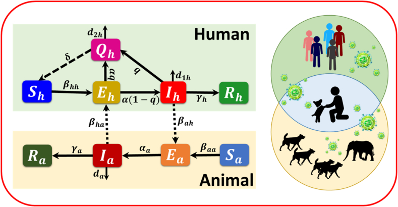
The present SEIR-based quarantined model $\left(S_h{E}_h{I}_h{Q}_h{R}_h{S}_a{E}_a{I}_a{R}_a\right)$ has been purposefully made clear for a community with a well-mixing and infinite population. By analyzing $R_0$ it has been confirmed that both endemic and disease-free equilibrium points are locally and globally stable. The model and its solution are positive and bound to the total population size $N\left(t\right)$ [50]. Considering all the factors, we also examined the Lyapunov function's first and second derivatives. The first derivative of the Lyapunov function provides information about the course of the illness, while the second derivative provides information about the propensity toward curvature. After that, the model is fractionalized by applying significant ABC fractional derivatives. In this study, we examine the impact of quarantine measures on the spread of epidemics using deterministic and fractional-order dynamical models. We aim to assess the accuracy with which these models represent disease patterns. The suggested methodology is evaluated using extensive numerical analysis to assess its practical applicability for deterministic and fractional order scenarios. The first analysis focuses on the influence of evolutionary game theory on quarantine strategy, examining several parameter settings to demonstrate the effects of quarantine cost, protection factor, information likelihood, and variations in animal-to-human and human-to-animal transmission rates. Ultimately, the discussion is on expanding the epidemic model to include the fractional-order model, considering quarantine as a factor in behavioral dynamics (see Fig. 1).

Fig. 1.

Illustration depicting the suggested epidemic model: In our suggested model, denoted as $S_h{E}_{h}I\_h{Q}_h{R}_h{S}_a{E}_a{I}_a{R}_a$, susceptible humans $\left(S_h\right)$ are infected with a disease transmission rate ${\beta }_{hh}$. The black arrows represent the transmission of the state from susceptible $\left(S_h\right)$ to exposed humans $\left(E_h\right)$ due to interaction with sick persons. Once individuals are exposed $\left(E_h\right)$ after being susceptible $\left(S_h\right)$, a portion of them get infected with a progression rate of $\alpha \left(1-q\right)$ and instantly transition to an infected state $\left(I_h\right)$. The proportion of persons still asymptomatic and have not been identified is captured by the quarantine rate $\alpha q$ and, after that, put in the compartment $\left(Q_h\right)$. Persons who carry diseases are classified as infected humans $\left(I_h\right)$. Some infected persons may be forcibly transferred to the compartment $\left(Q_h\right)$ at a $q$ rate. The susceptibility of persons brought to the compartment $\left(Q_h\right)$ implementing quarantine or self-isolation regulations is determined by the rate δ. Once an individual has recovered $\left(R_h\right)$, they are excluded from further consideration within the local timeline of the progressing pandemic. The situation for animal patches is similar, except for the quarantine policy.

6.1. Deterministic approach

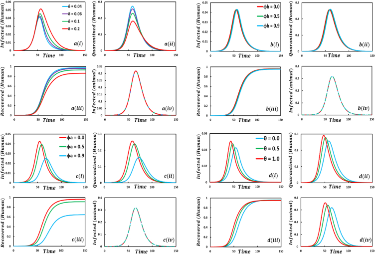
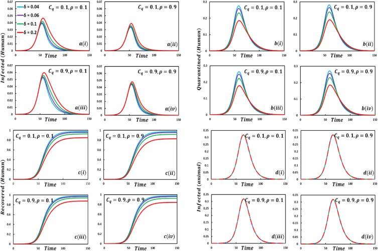
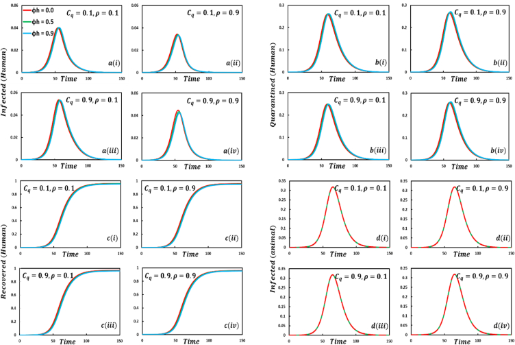
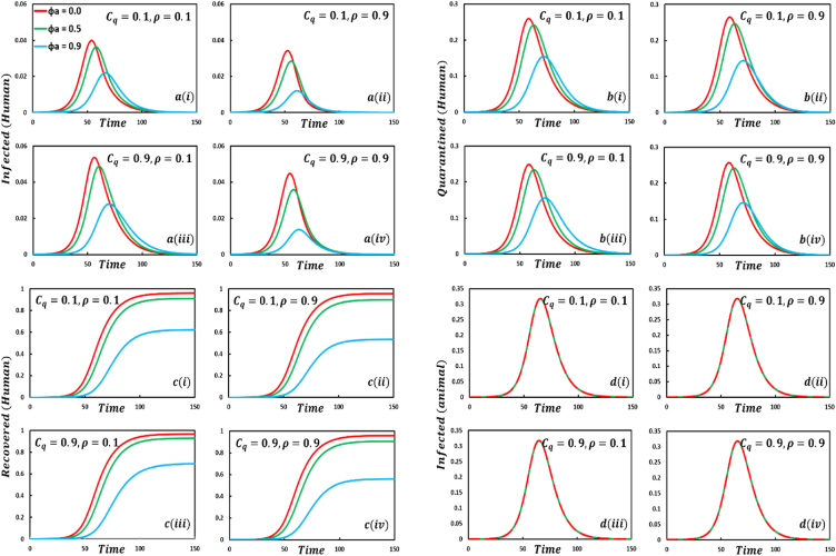
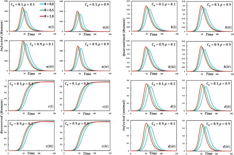
This subsection performs experiments under the most common parameter settings in Fig. 2, Fig. 3, Fig. 4, Fig. 5, Fig. 6, Fig. 7, Fig. 8, Fig. 9, Fig. 10, Fig. 11, Fig. 12, Fig. 13, Fig. 14, Fig. 15, Fig. 16, Fig. 17, Fig. 18 to explore the effects of evolutionary game theory and animal transmission on the spread of the human epidemic. Firstly, we simulate the proposed model by using the finite difference numerical scheme and demonstrate it through the time-evolving line graphs, considering a standard set of parameters termed the default case $({\mathrm{\Lambda }}_h=0,{\beta }_{hh}=1.0,{\phi }_a=0.0,{\phi }_h=0.0,{\delta }_h=0.06,{\mu }_h=0,{\alpha }_h=0.2,q=0.5,{\gamma }_h=0.1,{\mathrm{\Lambda }}_a=0.0,{\beta }_{aa}=0.5,\theta =0.0,{\mu }_a=0.0,{\alpha }_a=0.2and{\gamma }_a=0.1$) and changing values of the key parameters $\delta =0.04,0.06,0.1,0.2,{\phi }_h=0.0,0.5,0.9,{\phi }_a=0.0,0.5,0.9and\theta =0.0,0.5,1.0$ and respected dynamics are presented in Fig. 2 ($\delta \to \left(a^{*}\right)$, ${\phi }_h\to \left(b^{*}\right)$, ${\phi }_a\to \left(c^{*}\right)$ and $\theta \to \left(d^{*}\right)$, respectively). Secondly, we simulate the model for crucial parameters with four sets $\left(\left(Cq,\rho \right)=\left(0.1,0.1\right),\left(0.1,0.9\right),\left(0.9,0.1\right),\left(0.9,0.9\right)\right)$ of EGT techniques and varying the values of vital parameters as mentioned above, illustrated in Fig. 3, Fig. 4, Fig. 5, Fig. 6. In Figure $-2\left(a^{*}\right)$, we see that for increasing values of $\delta =0.04,0.06,0.1,0.2\text{,}$ the number of infected human curves shows an increasing trend. In addition, the opposite scenarios are for quarantined and recovered humans, whereas the number of infected animals is the same, and no fluctuation appears. When the quarantined people did not properly maintain the quarantine period, and after the quarantine period, they went back to the susceptible class. As a result, infected individuals increased rapidly, decreasing the number of quarantined and recovered humans. Another vital characteristic is that the quarantine duration did not affect animal infection. That is why the infected animal curve exhibits the same characteristics. For increasing values of ${\phi }_h=0.0,0.5,0.9$, (Figure $2\left(b^{*}\right)$ the number of infected, quarantined, and recovered humans and infected animals show a delaying tendency. It is evident that when people have enough protection to protect themselves from infected humans who transmit the monkeypox disease, disease dynamics show a slowing transmission curve but reveal the highest transmission peak but significantly less compared to subfigure $a\left(i\right)$. Due to the lack of proper treatment or vaccination, people firstly protect themselves from infected individuals. After a certain period, it collapses and discloses its maximum peak point of disease. As a result, the number of quarantined and recovered people is also lessened. Significant fluctuations of infected, quarantined, and recovered human curves are revealed for different values of the protection rate against infected animals ${\phi }_a=0.0,0.5,0.9\text{,}$ which is demonstrated in Figure $2\left(c^{*}\right)$. When people have no protection, many people are infected by mpox disease. Thus, quarantine and FES curves show increasing characteristics. In contrast, opposite scenarios for ${\phi }_a=0.9$, an expected outcome. Figure $2\left(d\left(i\right)-d\left(iv\right)\right)$ discloses that for increasing values of human-to-animal transmission rate, $\theta =0.0,0.5,1.0$, all compartments illustrate an uprising trend. Since numerous animal species are known to be susceptible to monkeypox, this scenario lends credence to the “WHO” warning that the mpox virus may transmit from people to vulnerable animal species in other habitats, perhaps creating new reservoirs. As a result, people with confirmed or suspected monkeypox should stay away from animals, whether they are domestic pets (including dogs, cats, hamsters, and gerbils), livestock, or wild animals [2]. Sophie et al. [63] findings proved the ‘WHO’ warning.

Fig. 2.

Presented the effect of $\left(a^{*}\right)$ Quarantine or self-isolation period, $\delta =0.04,0.06,0.1,0.2\text{,}$$\left(b^{*}\right)$ protection rate against infected humans, ${\phi }_h=0.0,0.5,0.9\text{,}$$\left(c^{*}\right)$ protection rate against infected animals, ${\phi }_a=0.0,0.5,0.9\text{,}$$\left(d^{*}\right)$ the transmission rate of human to animal, $\theta =0.0,0.5,1.0$ on the infected (human), quarantined (human), recovered (human) individuals, and infected animals. In the general case, the parameter setting is ${\beta }_{hh}=1.0,{\beta }_{aa}=0.5,{\phi }_h={\phi }_a=0.0,{\alpha }_h={\alpha }_a=0.2,{\gamma }_h={\gamma }_a=0.1,\delta =0.06,\theta =0.0\text{.}$.

Fig. 3.

Presented the effect of $\delta =0.04,0.06,0.1,0.2$ on the infected (human), quarantined (human), recovered (human) individuals, and infected animals. Subpanels $a\left(i\right),a\left(ii\right),a\left(iii\right)\text{,}$ and $a\left(iv\right)$ show the results under the quarantine cost and disease information probability $\left(C_q,\rho \right)=\left(0.1,0.1\right)\left(0.1,0.9\right),\left(0.9,0.1\right)$ and $\left(0.9,0.9\right)$, respectively, whereas the remaining parameter settings are ${\beta }_{hh}=1.0,{\beta }_{aa}=0.5,{\phi }_h={\phi }_a=0.0,{\alpha }_h={\alpha }_a=0.2,{\gamma }_h={\gamma }_a=0.1,\theta =0.0\text{.}$.

Fig. 4.

Presented the effect of ${\phi }_h=0.0,0.5,0.9$ on the infected (human), quarantined (human), recovered (human) individuals, and infected animals. Subpanels $b\left(i\right),b\left(ii\right),b\left(iii\right)\text{,}$ and $b\left(iv\right)$ show the results under the quarantine cost and disease information probability $\left(C_q,\rho \right)=\left(0.1,0.1\right)\left(0.1,0.9\right),\left(0.9,0.1\right)$ and $\left(0.9,0.9\right)$, respectively, whereas the remaining parameter settings are ${\beta }_{hh}=1.0,{\beta }_{aa}=0.5,{\phi }_a=0.0,{\alpha }_h={\alpha }_a=0.2,{\gamma }_h={\gamma }_a=0.1,\theta =0.0,\delta =0.06\text{.}$.

Fig. 5.

Presented the effect of ${\phi }_a=0.0,0.5,0.9$ on the infected (human), quarantined (human), recovered (human) individuals, and infected animals. Subpanels $c\left(i\right),c\left(ii\right),c\left(iii\right)\text{,}$ and $c\left(iv\right)$ show the results under the quarantine cost and disease information probability $\left(C_q,\rho \right)=\left(0.1,0.1\right)\left(0.1,0.9\right),\left(0.9,0.1\right)$ and $\left(0.9,0.9\right)$, respectively, whereas the remaining parameters setting are ${\beta }_{hh}=1.0,{\beta }_{aa}=0.5,{\phi }_h=0.0,{\alpha }_h={\alpha }_a=0.2,{\gamma }_h={\gamma }_a=0.1,\theta =0.0,\delta =0.06\text{.}$.

Fig. 6.

Presented the effect of $\theta =0.0,0.5,1.0$ on the infected (human), quarantined (human), recovered (human) individuals, and infected animals. Subpanels $d\left(i\right),d\left(ii\right),d\left(iii\right)\text{,}$ and $d\left(iv\right)$ show the results under the quarantine cost and disease information probability $\left(C_q,\rho \right)=\left(0.1,0.1\right)\left(0.1,0.9\right),\left(0.9,0.1\right)$ and $\left(0.9,0.9\right)$, respectively, whereas the remaining parameter settings are ${\beta }_{hh}=1.0,{\beta }_{aa}=0.5,{\phi }_h={\phi }_a=0.0,{\alpha }_h={\alpha }_a=0.2,{\gamma }_h={\gamma }_a=0.1,\delta =0.06\text{.}$.

Fig. 7.

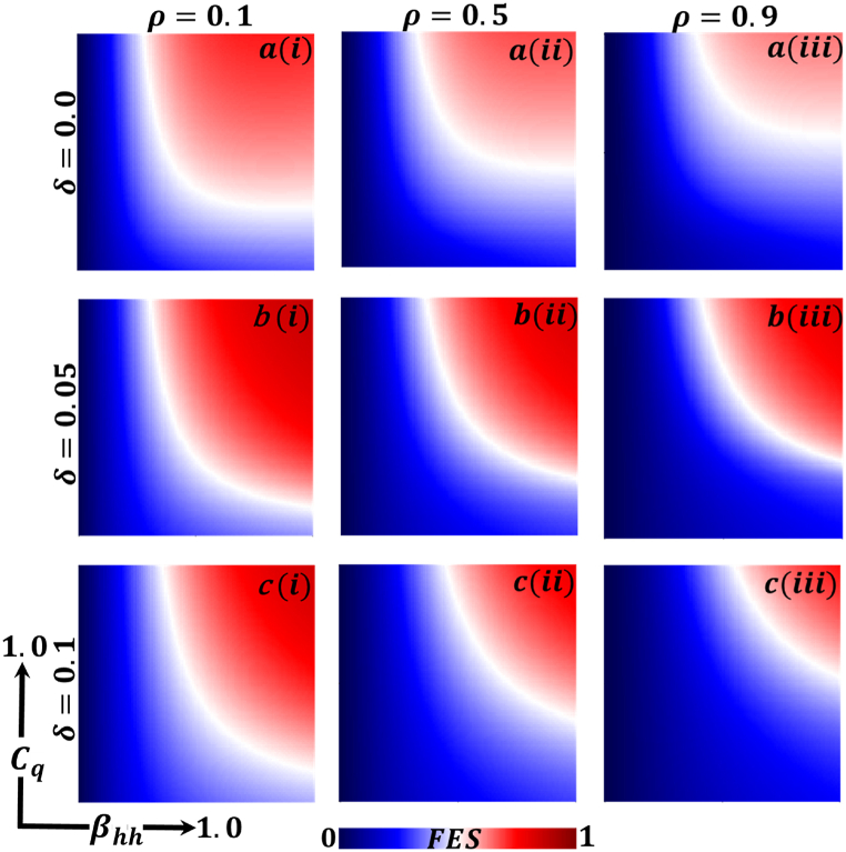
Presented the 2D heat maps of final epidemic size (FES) concerning the quarantine or self-isolation cost $\left(C_q\right)$ and human-to-human-transmission rate $\left({\beta }_{hh}\right)$. Subpanels (a*), (b*), and (c*) show the effect of quarantine or self-isolation period $\left(\delta =0.0,0.05and0.1\right)\text{,}$ whereas (*-i), (*-ii), (*-iii) represents the information probability of the infected animal $\left(\rho =0.1,0.5and0.9\right)$, respectively. The remaining parameter settings are ${\beta }_{aa}=0.5,{\phi }_h={\phi }_a=0.5,{\alpha }_h=0.2,{\alpha }_a=0.1,{\gamma }_h={\gamma }_a=0.2,\theta =0.5$.

Fig. 8.

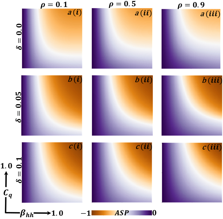
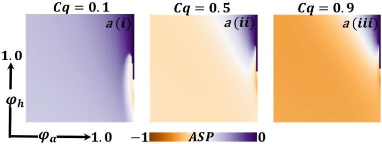
Presented the 2D heat maps of the average social payoff (ASP) concerning the quarantine or self-isolation cost $\left(C_q\right)$ and human-to-human-transmission rate $\left({\beta }_{hh}\right)$. Subpanels (a*), (b*), and (c*) show the effect of quarantine or self-isolation period $\left(\delta =0.0,0.05and0.1\right)\text{,}$ whereas (*-i), (*-ii), (*-iii) represents the information probability of the infected animal $\left(\rho =0.1,0.5and0.9\right)$, respectively. The remaining parameter settings are ${\beta }_{aa}=0.5,{\phi }_h={\phi }_a=0.5,{\alpha }_h=0.2,{\alpha }_a=0.1,{\gamma }_h={\gamma }_a=0.2,\theta =0.5$.

Fig. 9.

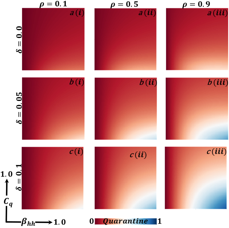
Presented the 2D heat maps of quarantine effect concerning the quarantine or self-isolation cost $\left(C_q\right)$ and human-to-human-transmission rate $\left({\beta }_{hh}\right)$. Subpanels (a*), (b*), and (c*) show the effect of quarantine or self-isolation period $\left(\delta =0.0,0.05and0.1\right)\text{,}$ whereas (*-i), (*-ii), (*-iii) represents the information probability of the infected animal $\left(\rho =0.1,0.5and0.9\right)$, respectively. The remaining parameter settings are ${\beta }_{aa}=0.5,{\phi }_h={\phi }_a=0.5,{\alpha }_h=0.2,{\alpha }_a=0.1,{\gamma }_h={\gamma }_a=0.2,\theta =0.5$.

Fig. 10.

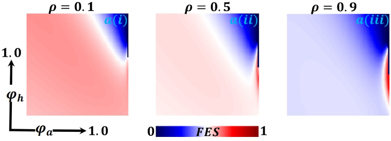
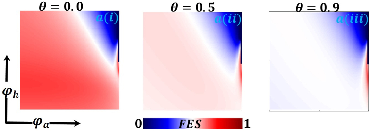
Presented the 2D heat maps of final epidemic size (FES) concerning the protection rate of infected animals $\left({\phi }_a\right)$ and the protection rate of infected humans $\left({\phi }_h\right)$. Subpanels $a^{*}$ show show the effect of the information probability of the infected animal $\left(\rho =0.1,0.5and0.9\right)$, respectively. The remaining parameter settings are ${{\beta }_{hh}=0.8333,\beta }_{aa}=0.5,C_q=0.5,{\alpha }_h=0.2,{\alpha }_a=0.1,{\gamma }_h={\gamma }_a=0.2,\theta =0.5$.

Fig. 11.

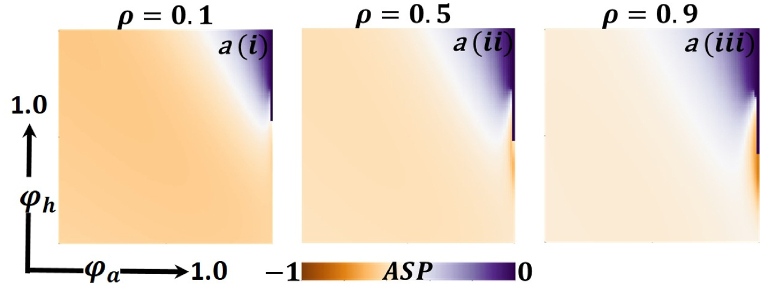
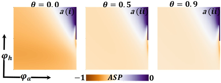
Presented the 2D heat maps of the average social payoff (ASP) concerning the protection rate of infected animals $\left({\phi }_a\right)$ and the protection rate of infected humans $\left({\phi }_h\right)$. Subpanels $a^{*}$ show the effect of the information probability of the infected animal $\left(\rho =0.1,0.5and0.9\right)$, respectively. The remaining parameter settings are ${{\beta }_{hh}=0.8333,\beta }_{aa}=0.5,C_q=0.5,{\alpha }_h=0.2,{\alpha }_a=0.1,{\gamma }_h={\gamma }_a=0.2,\theta =0.5$.

Fig. 12.

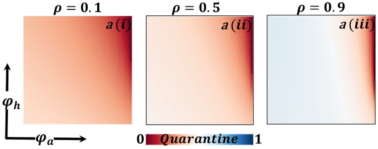
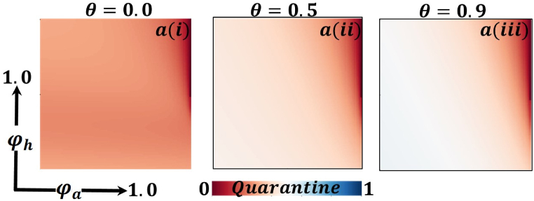
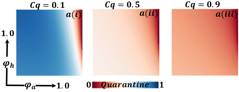
Presented the 2D heat maps of the quarantine effect concerning the protection rate of infected animals $\left({\phi }_a\right)$ and the protection rate of infected humans $\left({\phi }_h\right)$. Subpanels $a^{*}$ show the effect of information probability of the infected animal $\left(\rho =0.1,0.5and0.9\right)$, respectively. The remaining parameter settings are ${{\beta }_{hh}=0.8333,\beta }_{aa}=0.5,C_q=0.5,{\alpha }_h=0.2,{\alpha }_a=0.1,{\gamma }_h={\gamma }_a=0.2,\theta =0.5$.

Fig. 13.

Presented the 2D heat maps of final epidemic size (FES) concerning the protection rate of infected animals $\left({\phi }_a\right)$ and the protection rate of infected humans $\left({\phi }_h\right)$. Subpanels $a^{*}$ show the effect of the human-to-animal transmission rate $\left(\theta =0.0,0.5and0.9\right)$, respectively. The remaining parameter settings are ${{\beta }_{hh}=0.8333,\beta }_{aa}=0.5,C_q=0.5,{\alpha }_h=0.2,{\alpha }_a=0.1,{\gamma }_h={\gamma }_a=0.2,\rho =0.9$.

Fig. 14.

Presented the 2D heat maps of the average social payoff (ASP) concerning the protection rate of infected animals $\left({\phi }_a\right)$ and the protection rate of infected humans $\left({\phi }_h\right)$. Subpanels $a^{*}$ show the effect of the human-to-animal transmission rate $\left(\theta =0.0,0.5and0.9\right)$, respectively. The remaining parameters setting are ${{\beta }_{hh}=0.8333,\beta }_{aa}=0.5,C_q=0.5,{\alpha }_h=0.2,{\alpha }_a=0.1,{\gamma }_h={\gamma }_a=0.2,\rho =0.9$.

Fig. 15.

Presented the 2D heat maps of the quarantine effect concerning the protection rate of infected animals $\left({\phi }_a\right)$ and the protection rate of infected humans $\left({\phi }_h\right)$. Subpanels $a^{*}$ show the effect of the human-to-animal transmission rate $\left(\theta =0.0,0.5and0.9\right)$, respectively. The remaining parameter settings are ${{\beta }_{hh}=0.8333,\beta }_{aa}=0.5,C_q=0.5,{\alpha }_h=0.2,{\alpha }_a=0.1,{\gamma }_h={\gamma }_a=0.2,\rho =0.9$.

Fig. 16.

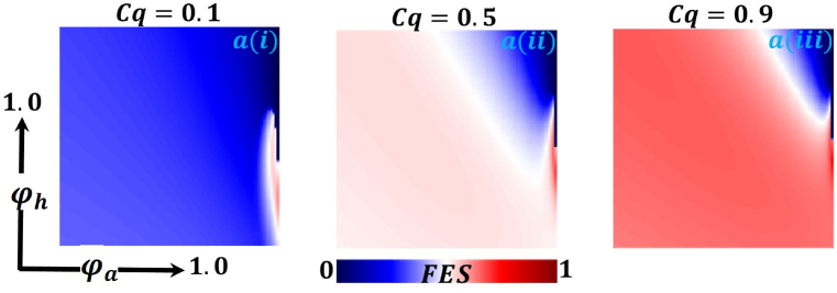
Presented the 2D heat maps of final epidemic size (FES) concerning the protection rate of infected animals $\left({\phi }_a\right)$ and the protection rate of infected humans $\left({\phi }_h\right)$. Subpanels $a^{*}$ show the effect of quarantine cost $\left(C_q=0.1,0.5and0.9\right)$, respectively. The remaining parameter settings are ${{\beta }_{hh}=0.8333,\beta }_{aa}=0.5,\theta =0.5,{\alpha }_h=0.2,{\alpha }_a=0.1,{\gamma }_h={\gamma }_a=0.2,\rho =0.9$.

Fig. 17.

Presented the 2D heat maps of average social payoff (ASP) concerning the protection rate of infected animals $\left({\phi }_a\right)$ and the protection rate of infected humans $\left({\phi }_h\right)$. Subpanels $a^{*}$ show the effect of quarantine cost $\left(C_q=0.1,0.5and0.9\right)$, respectively. The remaining parameter settings are ${{\beta }_{hh}=0.8333,\beta }_{aa}=0.5,\theta =0.5,{\alpha }_h=0.2,{\alpha }_a=0.1,{\gamma }_h={\gamma }_a=0.2,\rho =0.9$.

Fig. 18.

Presented the 2D heat maps of the quarantine effect concerning the protection rate of infected animals $\left({\phi }_a\right)$ and the protection rate of infected humans $\left({\phi }_h\right)$. Subpanels $a^{*}$ show the effect of quarantine cost $\left(C_q=0.1,0.5and0.9\right)$, respectively. The remaining parameter settings are ${{\beta }_{hh}=0.8333,\beta }_{aa}=0.5,\theta =0.5,{\alpha }_h=0.2,{\alpha }_a=0.1,{\gamma }_h={\gamma }_a=0.2,\rho =0.9$.

In Fig. 3, four strategies, namely sub-figures $\left(a^{*},b^{*},c^{*},d^{*}\right)$ of EGT $\left(\left(Cq,\rho \right)=\left(0.1,0.1\right),\left(Cq,\rho \right)=\left(0.1,0.9\right),\left(Cq,\rho \right)=\left(0.9,0.1\right),\left(Cq,\rho \right)=\left(0.9,0.9\right)\right)$ techniques demonstrate that the increasing values of the parameter $\delta$, exhibit mixed outcomes and expected results. When the self-quarantine cost $C_q=0.1$ for individuals, and the information probability of the infected animal $\left(\rho =0.1\right)$ is low; the number of infected individuals is also less compared to default case infected individuals, illustrated in sub-Fig. 3($a\left(i\right))$. The number of infected individuals is significantly less compared to default and $\left(Cq,\rho \right)=\left(0.1,0.1\right)$ case infected individuals for the values of $\left(Cq,\rho \right)=\left(0.1,0.9\right)\text{,}$ sub-Fig. 3($a\left(ii\right))$. Realistically, more information on infected animals with monkeypox diseases assists in reducing the transmission of the disease. But when the cost is more than the information probability $\left(Cq,\rho \right)=\left(0.9,0.1\right)$, sub-Fig. 3($a\left(iii\right))$, the disease will show a rising trend. In that scenario, people are not aware anymore, and due to the cost of quarantine, they are not too interested in going to quarantine. As a result, the number of infected individuals is rising. The fourth setting $\left(Cq,\rho \right)=\left(0.9,0.9\right)\text{,}$ sub-Fig. 3($a\left(iv\right))$, shows decreasing characteristics of the disease curve instead of high cost but enough information about the disease. The quarantine compartment indicates some remarkable features. In the first set, sub-Fig. 3($b\left(i\right))$, although information probability is low, more people will participate in quarantine because of low expenses. The second set, sub-Fig. 3($b\left(ii\right))$, displays fewer people participating in quarantine than the first because people are more cautious about the disease due to sufficient information, whereas, in the fourth set, sub-Fig. 3($b\left(iv\right))$, many people participate in quarantine because of the plethora of information about the infected animal, instead of high quarantine cost, a realistic outcome. Furthermore, if the quarantined people fully maintain the quarantine policy, they recover more. Such scenarios are illustrated in sub-Fig. 3($c^{*})$ for recovered individuals. Furthermore, the infected animal's infection curve sub-Fig. 3($d^{*})\text{,}$ show almost constant circumstances as human awareness and infection did not affect animal infection.

Fig. 4, sub-figures $\left(a^{*},b^{*},c^{*},d^{*}\right)$ displays that if humans have no protection against infected humans (${\phi }_h=0.0)$, the infected, quarantined, and recovered human curves exhibit an uprising and quick trend, whereas the infected animal curve has no change. On top of that, if humans have a shield against infected humans (${\phi }_h=0.5,0.9)$, the epidemic curve shows a delayed but high peak trend, even if the four compartmental curve size demonstrates a fluctuation tendency for different EGT strategies.

Disease dynamics of mpox disease are displayed in Fig. 5, sub-figures $\left(a^{*},b^{*},c^{*},d^{*}\right)$ in the context of increasing values of protection rate against infected animal ${\phi }_a=0.0,0.5,0.9\text{.}$ When people have no protection against infected animals (${\phi }_a=0.0)$, the infected, quarantined, and recovered human curves exhibit a rising disease characteristic, whereas previous type outcomes for the infected animal curve. It is undoubtedly true that if people have enough protection against the infected animal, mpox disease will be unable to show its devastating color among human societies before fading out.

Fig. 6, sub-figures $\left(a^{*},b^{*},c^{*},d^{*}\right)$ illustrates the possible outcomes of four strategies of EGT techniques corresponding to the increasing values of the control parameter $\theta$, the transmission rate of human to animal. When the value of $\theta =0\text{,}$ i.e., no infection will hold from human to animal, the infected, quarantine, recovered human, and infected animal curves demonstrate a lower and delayed peak curve in all EGT settings, realistic outcomes. Furthermore, increasing values of the transmission rate of human-to-animal displays an increasing trend and the highest epidemic peak at the earliest time frame, the reverse scenarios of no infection transmission case. The exact consequences for other compartments.

Now let us focus on the scenario where FES (final epidemic size), ASP (average social payoff), and quarantine are shown as a 2D phase diagram, Fig. 7, Fig. 8, Fig. 9, at equilibrium (t → ∞), considering ${\beta }_{h}vs.C_q$ ranging from 0 to 1 (FES & quarantine) and $-1$ to 0 (ASP). Furthermore, the FES, ASP, and Quarantine size for the quarantine period along the column direction ($\delta$ = 0.0,0.05 and 0.1) and the information probability of the infected animal along the row direction $\left(\rho =0.1,0.5and0.9\right)$ are illustrated in Fig. 7, Fig. 8, Fig. 9. When $\delta$ = 0.0, i.e., no quarantined people back to susceptible compartments, and the value of $\rho$ increases ($0.1,0.5and0.9)$ at a specific rate, the final epidemic size decreases gradually. Similar consequences for other cases ($\delta$ = 0.05 and 0.1), but for $\delta$ = 0.05, FES is more significant than the first case. It is realistic that when people have to maintain a 20-day quarantine period, some do not maintain all rules and regulations, which is the main reason for increasing FES. Finally, the FES decreased for $\delta$ = 0.1 and $\rho =0.1,0.5and0.9$. For the values of $\delta$ = 0.1 and $\rho =0.9$, the FES is much smaller than the DFE point. Fig. 8, Fig. 9 have similar display features. At the final setting of $\delta$ and $\rho \text{,}$ ASP increased an expected level, and a more significant portion of people participated in quarantine, reducing the FES of the epidemic. Fig. 10, Fig. 13, Fig. 16 illustrate the FES corresponding to the values of $\rho \left(0.1,0.5and0.9\right)\text{,}$ $\theta \left(0.0,0.5and0.9\right)$ and $Cq\left(0.1,0.5and0.9\right)\text{,}$ where ${\phi }_a$ and ${\phi }_h$ along the $x$ and $y$-axis, ranging from 0 to 1. For increasing values $\rho ,\theta \text{,}$ and $Cq$, the FES is reduced at a significant level where Fig. 16 displays reverse outcomes. Realistically, when people have enough information about the disease and the cost of quarantine is high, FES gradually declines for the first two cases, and for the third case, it will show a rising trend. Similarly, Fig. 11, Fig. 12, Fig. 14, Fig. 15, Fig. 17, Fig. 18 illustrate that ASP and quarantined 2D heat map exhibits the same characteristics as FES.

6.2. Fractional order approach

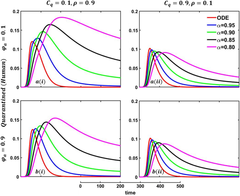
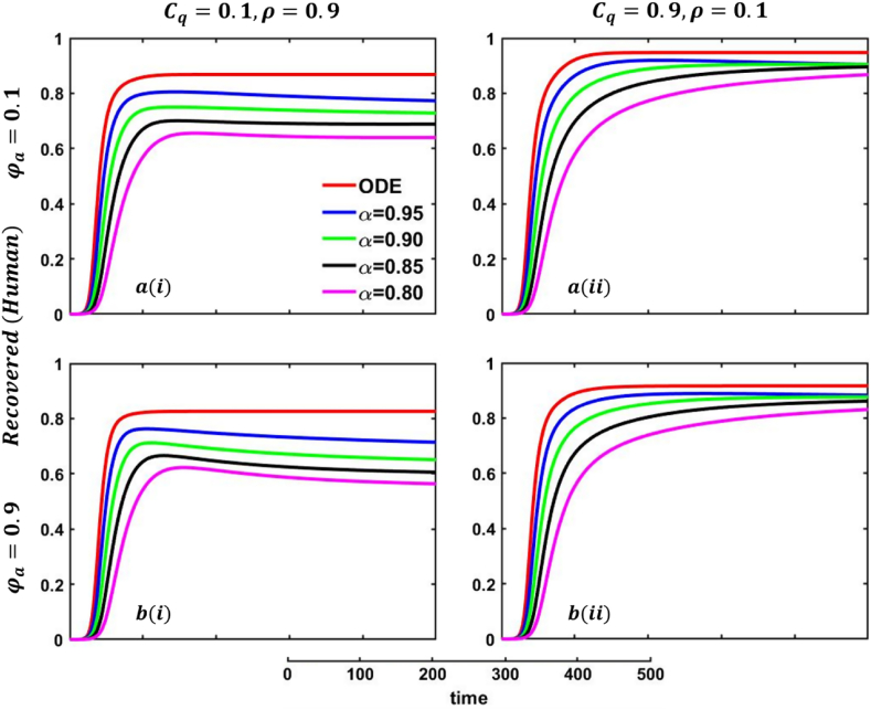
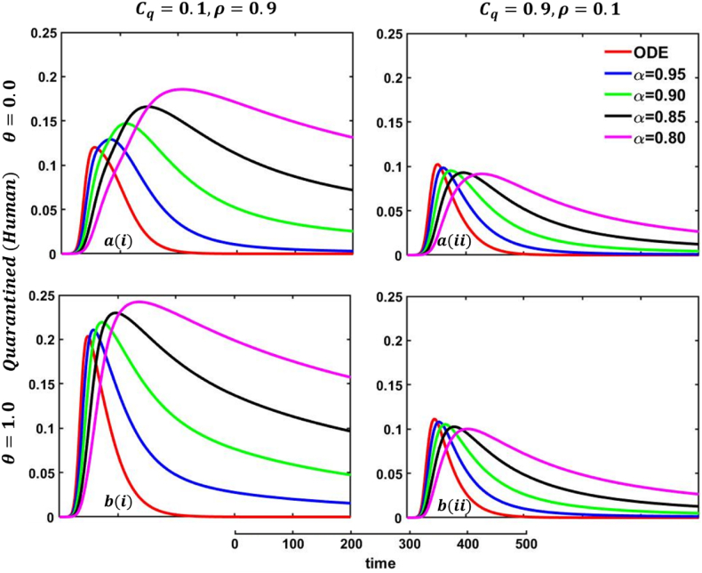
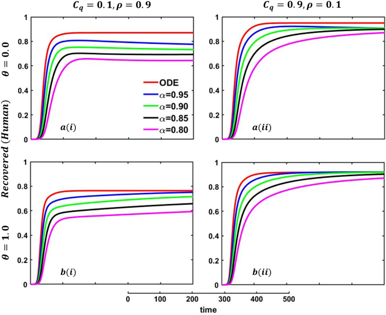
Driven by the above discussion, we describe a comprehensive analysis of the behavior taking quarantine and delay effect in fractional order models for different cases in Fig. 18, Fig. 19, Fig. 20, Fig. 21, Fig. 22, Fig. 23, Fig. 24, Fig. 25, Fig. 26, Fig. 27, Fig. 28 (Quarantine or self-isolation period, Protection rate against human and animal, and Transmission rate). Fig. 19, Fig. 20 illustrate the quarantine and recovered individuals’ overall fluctuating dynamics during the mpox disease, considering the EGT mechanisms $\left(\left(Cq,\rho \right)=\left(0.1,0.1\right),\left(Cq,\rho \right)=\left(0.1,0.9\right),\left(Cq,\rho \right)=\left(0.9,0.1\right),\left(Cq,\rho \right)=\left(0.9,0.9\right)\right)\text{,}$ with different fractional orders $\left(\alpha =1.0\left(ODE\right),0.95,0.90,0.85,0.80\right)$ employing non-singular and non-local kernels, namely, ABC fractional-order derivative, where parameters setting are ${\beta }_{hh}=1.0,{\beta }_{aa}=0.5,{\phi }_h={\phi }_a=0.0,{\alpha }_h={\alpha }_a=0.2,{\gamma }_h={\gamma }_a=0.1,\delta =0.04,\theta =0.0\text{.}$ In addition, Fig. 21, Fig. 22, Fig. 23, Fig. 24, Fig. 25, Fig. 26, Fig. 27, Fig. 28 demonstrate the disease dynamics of a different set of parameter values ${\delta ,\phi }_h,{\phi }_a,\theta$ with EGT strategies $\left(\left(Cq,\rho \right)=\left(0.1,0.9\right),\left(0.9,0.1\right)\right)$.

Fig. 19.

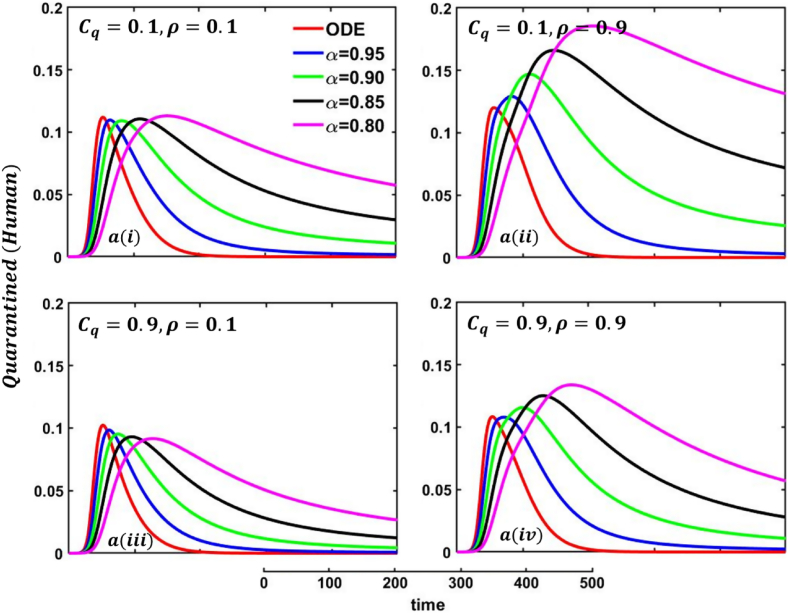
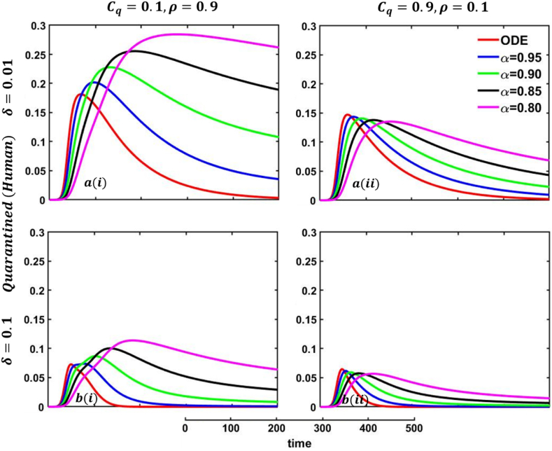
Explored the impact of altering the fractional-order $\alpha =1.0,0.95,0.9,0.85,0.8$ on the quarantined (human) individuals. Subpanels $a\left(i\right),a\left(ii\right),a\left(iii\right)\text{,}$ and $a\left(iv\right)$ show the results under the quarantine cost and disease information probability $\left(C_q,\rho \right)=\left(0.1,0.1\right)\left(0.1,0.9\right),\left(0.9,0.1\right)$ and $\left(0.9,0.9\right)$, respectively, whereas the remaining parameter settings are ${\beta }_{hh}=1.0,{\beta }_{aa}=0.5,{\phi }_h={\phi }_a=0.0,{\alpha }_h={\alpha }_a=0.2,{\gamma }_h={\gamma }_a=0.1,\delta =0.04,\theta =0.0$.

Fig. 20.

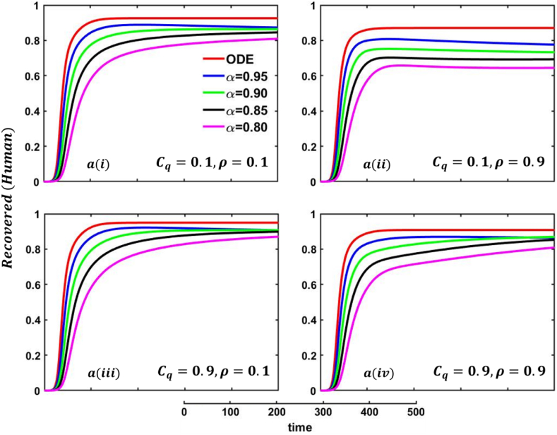
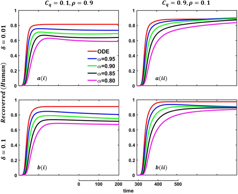
Explored the impact of altering the fractional-order $\alpha =1.0,0.95,0.9,0.85,0.8$ on the recovered (human) individuals. Subpanels $a\left(i\right),a\left(ii\right),a\left(iii\right)\text{,}$ and $a\left(iv\right)$ show the results under the quarantine cost and disease information probability $\left(C_q,\rho \right)=\left(0.1,0.1\right)\left(0.1,0.9\right),\left(0.9,0.1\right)$ and $\left(0.9,0.9\right)$, respectively, whereas the remaining parameter settings are ${\beta }_{hh}=1.0,{\beta }_{aa}=0.5,{\phi }_h={\phi }_a=0.0,{\alpha }_h={\alpha }_a=0.2,{\gamma }_h={\gamma }_a=0.1,\delta =0.04,\theta =0.0$.

Fig. 21.

Explored the impact of altering the fractional-order $\alpha =1.0,0.95,0.9,0.85,0.8$ on the quarantined (human) individuals. Subpanels (*-i) and (*-ii) show the results under the quarantine cost and disease information probability $\left(C_q,\rho \right)=\left(0.1,0.9\right)$ and $\left(0.9,0.1\right)\text{.}$ Subpanels (a*) and (b*) show the results under the quarantine period $\delta =0.01$ and $0.1\text{,}$ respectively, whereas the remaining parameters settings are ${\beta }_{hh}=1.0,{\beta }_{aa}=0.5,{\phi }_a={\phi }_h=0.0,{\alpha }_h={\alpha }_a=0.2,{\gamma }_h={\gamma }_a=0.1,\theta =0.0$.

Fig. 22.

Explored the impact of altering the fractional-order $\alpha =1.0,0.95,0.9,0.85,0.8$ on the recovered (human) individuals. Subpanels (*-i) and (*-ii) show the results under the quarantine cost and disease information probability $\left(C_q,\rho \right)=\left(0.1,0.9\right)$ and $\left(0.9,0.1\right)\text{.}$ Subpanels (a*) and (b*) show the results under the quarantine period $\delta =0.01$ and $0.1\text{,}$ respectively, whereas the remaining parameters settings are ${\beta }_{hh}=1.0,{\beta }_{aa}=0.5,{\phi }_a={\phi }_h=0.0,{\alpha }_h={\alpha }_a=0.2,{\gamma }_h={\gamma }_a=0.1,\theta =0.0$.

Fig. 23.

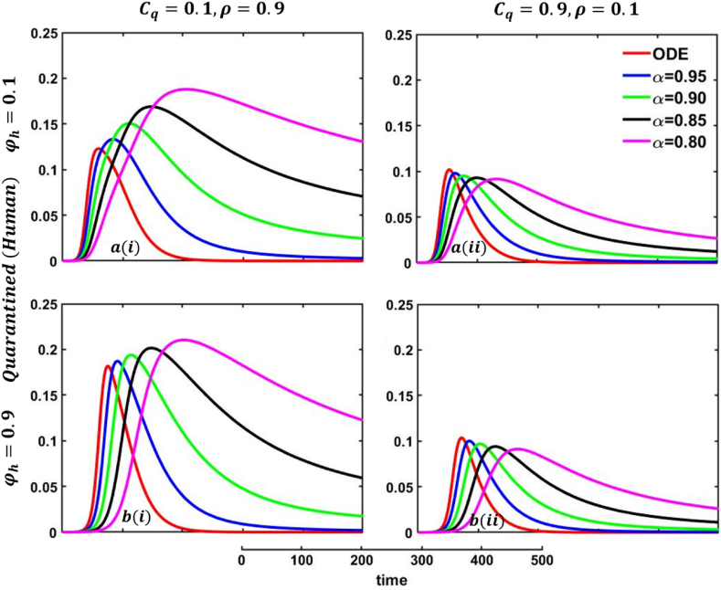
Explored the impact of altering the fractional-order $\alpha =1.0,0.95,0.9,0.85,0.8$ on the quarantined (human) individuals. Subpanels (*-i) and (*-ii) show the results under the quarantine cost and disease information probability $\left(C_q,\rho \right)=\left(0.1,0.9\right)$ and $\left(0.9,0.1\right)\text{.}$ Subpanels (a*) and (b*) show the results under the protection rate against infected human ${\phi }_h=0.1$ and $0.9\text{,}$ respectively, whereas the remaining parameter settings are ${\beta }_{hh}=1.0,{\beta }_{aa}=0.5,{\phi }_a=0.0,{\alpha }_h={\alpha }_a=0.2,{\gamma }_h={\gamma }_a=0.1,\delta =0.04,\theta =0.0$.

Fig. 24.

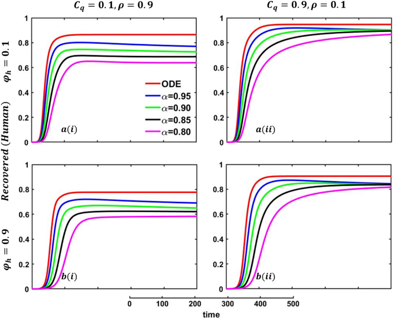
Explored the impact of altering the fractional-order $\alpha =1.0,0.95,0.9,0.85,0.8$ on the recovered (human) individuals. Subpanels (*-i) and (*-ii) show the results under the quarantine cost and disease information probability $\left(C_q,\rho \right)=\left(0.1,0.9\right)$ and $\left(0.9,0.1\right)\text{.}$ Subpanels (a*) and (b*) show the results under the protection rate against infected human ${\phi }_h=0.1$ and $0.9\text{,}$ respectively, whereas the remaining parameter settings are ${\beta }_{hh}=1.0,{\beta }_{aa}=0.5,{\phi }_a=0.0,{\alpha }_h={\alpha }_a=0.2,{\gamma }_h={\gamma }_a=0.1,\delta =0.04,\theta =0.0$.

Fig. 25.

Explored the impact of altering the fractional-order $\alpha =1.0,0.95,0.9,0.85,0.8$ on the quarantined (human) individuals. Subpanels (*-i) and (*-ii) show the results under the quarantine cost and disease information probability $\left(C_q,\rho \right)=\left(0.1,0.9\right)$ and $\left(0.9,0.1\right)\text{.}$ Subpanels (a*) and (b*) show the results under the protection rate against infected animal ${\phi }_a=0.1$ and $0.9\text{,}$ respectively, whereas the remaining parameter settings are ${\beta }_{hh}=1.0,{\beta }_{aa}=0.5,{\phi }_h=0.0,{\alpha }_h={\alpha }_a=0.2,{\gamma }_h={\gamma }_a=0.1,\delta =0.04,\theta =0.0$.

Fig. 26.

Explored the impact of altering the fractional-order $\alpha =1.0,0.95,0.9,0.85,0.8$ on the recovered (human) individuals. Subpanels (*-i) and (*-ii) show the results under the quarantine cost and disease information probability $\left(C_q,\rho \right)=\left(0.1,0.9\right)$ and $\left(0.9,0.1\right)\text{.}$ Subpanels (a*) and (b*) show the results under the protection rate against infected animal ${\phi }_a=0.1$ and $0.9\text{,}$ respectively, whereas the remaining parameter settings are ${\beta }_{hh}=1.0,{\beta }_{aa}=0.5,{\phi }_h=0.0,{\alpha }_h={\alpha }_a=0.2,{\gamma }_h={\gamma }_a=0.1,\delta =0.04,\theta =0.0$.

Fig. 27.

Explored the impact of altering the fractional-order $\alpha =1.0,0.95,0.9,0.85,0.8$ on the quarantined (human) individuals. Subpanels (*-i) and (*-ii) show the results under the quarantine cost and disease information probability $\left(C_q,\rho \right)=\left(0.1,0.9\right)$ and $\left(0.9,0.1\right)\text{.}$ Subpanels (a*) and (b*) show the results under the human-to-animal transmission rate $\theta =0.0$ and $1.0\text{,}$ respectively, whereas the remaining parameter settings are ${\beta }_{hh}=1.0,{\beta }_{aa}=0.5,{\phi }_h={\phi }_a=0.0,{\alpha }_h={\alpha }_a=0.2,{\gamma }_h={\gamma }_a=0.1,\delta =0.04$.

Fig. 28.

Explored the impact of altering the fractional-order $\alpha =1.0,0.95,0.9,0.85,0.8$ on the recovered (human) individuals. Subpanels (*-i) and (*-ii) show the results under the quarantine cost and disease information probability $\left(C_q,\rho \right)=\left(0.1,0.9\right)$ and $\left(0.9,0.1\right)\text{.}$ Subpanels (a*) and (b*) show the results under the human-to-animal transmission rate $\theta =0.0$ and $1.0\text{,}$ respectively, whereas the remaining parameter settings are ${\beta }_{hh}=1.0,{\beta }_{aa}=0.5,{\phi }_h={\phi }_a=0.0,{\alpha }_h={\alpha }_a=0.2,{\gamma }_h={\gamma }_a=0.1,\delta =0.04$.

In Fig. 21, Fig. 22, sub-figure $a\left(i\right)$ reveals that when the self-quarantine cost $C_q=0.1$, and the information probability of the infected animal $\left(\rho =0.1\right)$ both are low, with a small number of individuals going to quarantine. As a result, the FES size is significant due to the higher rate of infections. Reverse scenarios for the higher value of $\rho =0.9$, illustrated in Fig. 19, Fig. 20, sub-figure $a\left(ii\right)\text{,}$ whereas, $C_q=0.1\text{.}$ On top of that, it is well established that a lower-order fractional value generally delays the system; as a result, the disease curve takes more time to reach the peak. Such characteristics are revealed for lower-order fractional values, specifically for $\alpha =0.8$ (magenta color). Sub-figures $a\left(iii\right)$ and $a\left(iv\right)$ almost show the same but little bit lower tendency compared to sub-figures $a\left(i\right)$ and $a\left(ii\right)$, as an expected outcome.

6.3. Impact of quarantine or self-isolation period $\left({\delta }_h\right)$

In any epidemiological or pandemic time, if no perfect vaccination and anti-viral treatment are available, non-pharmaceutical intervention like quarantine or self-isolation is among the best unspoken measures to combat the disease. As of presently, for mpox virus disease scenarios, no perfect vaccination and anti-viral treatment are available, so if exposed and infected people flawlessly maintain the quarantine or self-isolation rules and regulations, then mpox disease would be under control and finally fade out without showing any devastating scenarios. Thus, if per day, 0.01% of people go back to the susceptible compartment from the quarantined compartment (illustrated in Fig. 19, sub-figure $a\left(i\right)-a\left(ii\right))$, then FES of Fig. 20, sub-figure $a\left(i\right)$ is small compared to Fig. 20, sub-figure $a\left(ii\right)$. Fig. 20, sub-figures $b\left(i\right)$ and $b\left(ii\right)$ revealed the same scenarios as sub-figure $a\left(i\right)$ and $a\left(ii\right)$ when per day, 0.5% of people go back to the susceptible compartment from the quarantined compartment.

6.4. Impact of protection rate against infected humans $\left({\phi }_h\right)$

One of the most crucial issues in controlling any epidemic disease is its transmission, which could be easily possible if we can control infected people to maintain the quarantine or self-isolation policy voluntarily or by force. Suppose the infected people have sufficient information about the disease and are aware (did not go to close a contract with another family member or a familiar or unfamiliar one) of the transmission. In that case, they and their respective societies are safe from any epidemic or pandemic. On top of that, if there are not enough preventive measures, namely, vaccination or effective anti-viral treatment, then controlling infected individuals would be the highest priority. Otherwise, society has to face a devastating scenario. In that case, quarantine and adequate disease information are the best alternatives for infected individuals and policymakers. Such type of scenarios are illustrated in Fig. 23, Fig. 24, sub-figures $\left(a\left(i\right)-a\left(ii\right),b\left(i\right)-b\left(ii\right)\right)\text{.}$ When people have fewer protection measures, but the quarantine cost is low and a higher rate of information provability about the disease, many participate in quarantine or self-isolation. As a result, the disease curve, as well as the recovered curve, show a decreasing tendency as an expected outcome, demonstrated in Fig. 23, Fig. 24, sub-figures $a\left(i\right)\text{.}$ In addition, the lower-order fractional-order curve (magenta color) is at the top due to the non-parasitical policy of quarantine or self-isolation due to the characteristics of fractional derivative. Opposite scenarios for sub-figures $a\left(ii\right)$ because of the high cost of quarantine and lower information rate; furthermore, if people have substantial protection measures against infected people and huge information compared to quarantine cost, they are not interested in any policy. Therefore, both the quarantined and recovered curves show a decreasing tendency, represented in Fig. 23, Fig. 24, sub-figures $b\left(i\right)$. Fig. 23, Fig. 24, sub-figures $b\left(ii\right)$ revealed the same scenarios as sub-figure $a\left(ii\right)$.

6.5. Impact of protection rate against infected animals $\left({\phi }_a\right)$

One of the most efficient strategies to reduce the probability of transmittable mpox from another animal is to avoid unprotected contact with wild animals (including their meat and blood), particularly those sick or dead. People can become infected with mpox if they come into direct physical contact with an infected animal, such as a non-human primate, terrestrial rodent, antelope, gazelle, or tree squirrel, which can happen through bites or scratches or when they engage in activities such as hunting, skinning, trapping, cooking, or playing with carcasses. Mpox can also be transmitted through sexual contact with an infected individual. It is also possible to get the virus by consuming infected animals that have not been adequately prepared before consumption. Any meal that contains animal parts or flesh needs to be fully prepared before being consumed in nations where monkeypox is common among the animal population. As a result, mpox virus carriers or infected animal control is another effective strategy to stop mpox disease transmission in our society. In that case, the policymaker's strict steps and self-awareness of individuals play an essential role. Therefore, when people have fewer protection measures against infected animals, with low quarantine cost and a higher rate of information provability about the disease, many people participate in quarantine or self-isolation, represented in Fig. 25, Fig. 26, sub-figures $a\left(i\right)$. In conclusion, Fig. 25, Fig. 26 revealed the same outcomes as those of Fig. 23, Fig. 24.

6.6. Impact of the transmission rate of human to animal $\left(\theta \right)$

Fig. 27, Fig. 28, sub-figures $\left(a\left(i\right)-a\left(ii\right),b\left(i\right)-b\left(ii\right)\right)$ exemplifies the possible outcomes of two strategies $\left(\left(Cq,\rho \right)=\left(0.1,0.9\right),\left(0.9,0.1\right)\right)$ of EGT techniques corresponding to the increasing values of the transmission rate of human to animal parameter $\theta$ with different fractional order. When the value of $\theta =0.0\text{,}$ i.e., no infection will hold from human to animal, and $\left(Cq,\rho \right)=\left(0.1,0.9\right)$, the human quarantine curve with different fractional order demonstrates that fewer people participate in quarantine or self-isolation (Fig. 27, sub-figure $(a\left(i\right)$) due to less infection. In addition, Fig. 27, sub-figure $a\left(ii\right)$ express that too few people participate in quarantine or self-isolation because of high quarantine costs and poor information provability compared to Fig. 27, sub-figure $(a\left(i\right)$. On top of that, the FES of Fig. 28, sub-figure $a\left(ii\right)$ is more significant than Fig. 28, sub-figure $a\left(i\right)$. Furthermore, increasing values of the transmission rate of human-to-animal with fractional order and EGT display an increasing trend for quarantine and a decreasing trend for FES, the reverse scenarios of no infection transmission case.

7. Conclusion

The rapid expansion of the mpox virus across many parts of the globe has resulted in a rise in the severity of the disease. Consequently, it is of the utmost necessity to comprehend the dynamics of this viral infection within an adaptable framework to provide more accurate findings. As a result, a nine-compartmental quarantined-based model in the presence of an EGT mechanism to describe the dynamics of mpox disease in humans and animals is constructed in this paper. Our research focused primarily on the qualitative analysis and the dynamic behavior of the mpox viral infection. First, we have presented the existence, uniqueness, non-negativity, and boundedness of the solution of the system of an ordinary differential equation. Within the context of Banach's, the fixed-point theorem is used to investigate whether the solution to the proposed fractional-order system for the mpox virus is unique and whether or not it even exists. In addition, we have investigated the local and global stability of the model through the basic equilibrium thresholds of the disease and Ulam-Hyers stability for the fractional order model.

Our numerical findings, utilizing mean-field and fractional-order approaches with Evolutionary Game Theory (EGT), shed light on the dynamic behavior of the mpox system. Unlike COVID-19, non-pharmaceutical interventions, especially quarantine-based models like IG, have proven highly effective in containing the disease. Quarantine policies significantly slow epidemic transmission, making them pivotal in combating mpox. Lower-order fractional orders also delay the epidemic peak, reinforcing their utility in modeling mpox dynamics. We observed that higher quarantine costs deter people from complying with quarantine measures, leading to an uptick in disease cases due to inadequate treatment and vaccination. Strict adherence to quarantine policies emerges as a critical factor in mpox control. Additionally, information about the disease plays a crucial role. When people are well-informed about the disease, they take preventive measures to reduce its spread. Protection against infected humans initially slows the epidemic but wanes over time, emphasizing the need for treatments and vaccines. Protection against infected animals is also vital. Adequate protection slows disease transmission, while a high human-to-animal transmission rate poses a catastrophic scenario. Avoiding close contact with all animals, including pets and livestock, is advised to prevent animal reservoirs. Lower-order fractional values delay the quarantine curve, extending the time to reach the peak.

Theoretical and numerical analysis of these models will guide us in effectively managing non-pharmaceutical interventions when a perfect vaccine is unavailable, preventing disease spread, and averting animal reservoirs. This research will also assist decision-makers in devising optimal strategies to address these critical situations. Refraining from close contact with animals, including pets and livestock, is recommended to avoid such dire situations. Overall, this research contributes to our understanding of complex epidemics, biological systems, and human behavior, providing valuable insights for managing disease outbreaks when a perfect vaccine is unavailable.

Fundings

This study has no funding.

Data availability statement

No data was used for the research described in the article.

CRediT authorship contribution statement

Mohammad Sharif Ullah: Writing – original draft, Visualization, Software, Methodology, Investigation, Formal analysis, Data curation, Conceptualization. K.M. Ariful Kabir: Writing – review & editing, Visualization, Supervision, Resources, Methodology, Investigation, Formal analysis, Conceptualization.

Declaration of competing interest

The authors declare that they have no known competing financial interests or personal relationships that could have appeared to influence the work reported in this paper.

References

- 1.Monkeypox, https://www.cdc.gov/poxvirus/monkeypox/about/index.html.
- 2.Monkeypox, https://www.who.int/health-topics/monkeypox#tab=tab_1.
- 3.Centers for Disease Control and Prevention . Division of High-Consequence Pathogens and Pathology (DHCPP) 2021. National center for emerging and zoonotic infectious diseases(NCEZID)https://www.cdc.gov/poxvirus/monkeypox/index.html Monkeypox. [Google Scholar]
- 4.Durski K.N., McCollum A.M., Nakazawa Y., Petersen B.W., Reynolds M.G., Briand S., Djingarey M.H., Olson V., Damon I.K., Khalakdina A. 2018. Emergence of Monkeypox West and Central Africa, 1970-2017 Morbidity and Mortality Weekly Report 67 306. [DOI] [PMC free article] [PubMed] [Google Scholar]
- 5.Jeźek Z., Szczeniowski M., Paluku K.M., Mutombo M., Grab B. Human monkeypox: confusion with chickenpox. PubMed. 1988;45(4):297–307. https://pubmed.ncbi.nlm.nih.gov/2907258 [PubMed] [Google Scholar]
- 6.Alakunle E.F., Moens U., Nchinda G., Okeke M.I. Monkeypox virus in Nigeria: infection biology, Epidemiology, and evolution. Viruses. 2020;12(11):1257. doi: 10.3390/v12111257. [DOI] [PMC free article] [PubMed] [Google Scholar]
- 7.Peter O.J., Kumar S., Kumari N., Oguntolu F.A., Oshinubi K., Rabiu M. Transmission dynamics of Monkeypox virus: a mathematical modelling approach. Modeling Earth Systems and Environment. 2021;8(3):3423–3434. doi: 10.1007/s40808-021-01313-2. [DOI] [PMC free article] [PubMed] [Google Scholar]
- 8.Bhunu C.P., Mushayabasa S. Modelling the transmission dynamics of pox-like infections. IAENG International Journal. 2011;41:1. –9. [Google Scholar]
- 9.Peter O.J., Kumar S., Kumari N., Oguntolu F.A., Oshinubi K., Rabiu M. Transmission dynamics of Monkeypox virus: a mathematical modelling approach. Modeling Earth Systems and Environment. 2021;8(3):3423–3434. doi: 10.1007/s40808-021-01313-2. [DOI] [PMC free article] [PubMed] [Google Scholar]
- 10.Peter O.J., Qureshi S., Yusuf A., Al-Shomrani M.M., Abioye A.I. A new mathematical model of COVID-19 using real data from Pakistan. Results Phys. 2021;24 doi: 10.1016/j.rinp.2021.104098. [DOI] [PMC free article] [PubMed] [Google Scholar]
- 11.Ojo M.M., Gbadamosi B., Olukayode A., Oluwaseun O.R. Sensitivity analysis of dengue model with saturated incidence rate. OAlib. 2018;5(3):1–17. doi: 10.4236/oalib.1104413. [DOI] [Google Scholar]
- 12.Idowu A.A., Olanrewaju I.M., Peter O.J., Sylvanus A., Abiodun O.F. Differential transform method for solving mathematical model of SEIR and SEI spread of malaria. Int. J. Sci. Basic Appl. Res. 2018;40(1):197–219. https://www.gssrr.org/index.php/JournalOfBasicAndApplied/article/download/9068/4079 [Google Scholar]
- 13.Kabir K.M.A., Islam M.S., Ullah M.S. Understanding the impact of vaccination and Self-Defense measures on epidemic dynamics using an embedded optimization and evolutionary game theory methodology. Vaccines. 2023;11(9):1421. doi: 10.3390/vaccines11091421. [DOI] [PMC free article] [PubMed] [Google Scholar]
- 14.Alam M., Kabir K.M.A., Tanimoto J. Based on mathematical epidemiology and evolutionary game theory, which is more effective: quarantine or isolation policy? J. Stat. Mech. Theor. Exp. 2020;2020(3) doi: 10.1088/1742-5468/ab75ea. [DOI] [Google Scholar]
- 15.Olumuyiwa P., Ibrahim M.O., Oguntolu F.A., Akinduko O.B., Akinyemi S.T. Direct and indirect transmission dynamics of Typhoid fever model by differential transform Method. ATBU Journal of Science, Technology and Education. 2018;6(1):167–177. https://www.atbuftejoste.com/index.php/joste/article/download/424/pdf_327 [Google Scholar]
- 16.Bankuru S.V., Kossol S., Hou W., Mahmoudi P., Rychtář J., Taylor D. A game-theoretic model of Monkeypox to assess vaccination strategies. PeerJ. 2020;8 doi: 10.7717/peerj.9272. [DOI] [PMC free article] [PubMed] [Google Scholar]
- 17.Usman S., Adamu I.I. Modeling the transmission dynamics of the monkeypox virus infection with treatment and vaccination interventions. J. Appl. Math. Phys. 2017;5(12):2335–2353. doi: 10.4236/jamp.2017.512191. [DOI] [Google Scholar]
- 18.Riaz A. Monkeypox and its outbreak. Pakistan Biomedical Journal. 2022;2 doi: 10.54393/pbmj.v5i8.792. [DOI] [Google Scholar]
- 19.Focosi D., Novazzi F., Baj A., Maggi F. Monkeypox: an international epidemic. Rev. Med. Virol. 2022;32(6) doi: 10.1002/rmv.2392. [DOI] [PubMed] [Google Scholar]
- 20.Ola P. Preprint; 2022. Monkeypox Is the Manifestation of Spectral Diseases and Not of Monkeypox Virus Transmission. [DOI] [Google Scholar]
- 21.Maruotti A., Böhning D., Rocchetti I., Ciccozzi M. Estimating the undetected infections in the Monkeypox outbreak. J. Med. Virol. 2022;95(1) doi: 10.1002/jmv.28099. [DOI] [PMC free article] [PubMed] [Google Scholar]
- 22.Damon I.K. ASM Press eBooks; 2014. Monkeypox Virus: Insights on its Emergence in Human Populations; pp. 85–97. [DOI] [Google Scholar]
- 23.Islam M.R., Hasan M., Rahman M.S., Rahman M.A. Monkeypox outbreak – No panic and stigma; Only awareness and preventive measures can halt the pandemic turn of this epidemic infection. Int. J. Health Plann. Manag. 2022;37(5):3008–3011. doi: 10.1002/hpm.3539. [DOI] [PubMed] [Google Scholar]
- 24.Peter O.J., Madubueze C.E., Ojo M.M., Oguntolu F.A., Ayoola T.A. Modeling and optimal control of monkeypox with cost-effective strategies. Modeling Earth Systems and Environment. 2022;9(2):1989–2007. doi: 10.1007/s40808-022-01607-z. [DOI] [Google Scholar]
- 25.Qurashi M.A., Rashid S., Alshehri A., Jarad F., Safdar F. New numerical dynamics of the fractional monkeypox virus model transmission pertaining to nonsingular kernels. Math. Biosci. Eng. 2022;20(1):402–436. doi: 10.3934/mbe.2023019. [DOI] [PubMed] [Google Scholar]
- 26.Owolabi K.M. Behavioural study of symbiosis dynamics via the Caputo and Atangana–Baleanu fractional derivatives. Chaos, Solit. Fractals. 2019;122:89–101. doi: 10.1016/j.chaos.2019.03.014. [DOI] [Google Scholar]
- 27.Higazy M., Allehiany F., Mahmoud E.E. Numerical study of fractional order COVID-19 pandemic transmission model in context of ABO blood group. Results Phys. 2021;22 doi: 10.1016/j.rinp.2021.103852. [DOI] [PMC free article] [PubMed] [Google Scholar]
- 28.Mouaouine A., Boukhouima A., Hattaf K., Yousfi N. A fractional order SIR epidemic model with nonlinear incidence rate. Adv. Differ. Equ. 2018;2018(1):1–9. doi: 10.1186/s13662-018-1613-z. [DOI] [Google Scholar]
- 29.Acay B., Berhe H.W., Yusuf A., Khan A., Yao S. Analysis of novel fractional COVID-19 model with real-life data application. Results Phys. 2021;23 doi: 10.1016/j.rinp.2021.103968. [DOI] [PMC free article] [PubMed] [Google Scholar]
- 30.Higazy M., Alyami M.A. New Caputo-Fabrizio fractional order SEIASqEqHR model for COVID-19 epidemic transmission with genetic algorithm based control strategy. Alex. Eng. J. 2020;59(6):4719–4736. doi: 10.1016/j.aej.2020.08.034. [DOI] [Google Scholar]
- 31.Shah K., Arfan M., Ullah A., Al‐Mdallal Q.M., Ansari K.J., Abdeljawad T. Computational study on the dynamics of fractional order differential equations with applications. Chaos, Solit. Fractals. 2022;157 doi: 10.1016/j.chaos.2022.111955. [DOI] [Google Scholar]
- 32.Ahmad S., Ullah A., Al‐Mdallal Q.M., Khan H., Shah K., Khan A. Fractional order mathematical modeling of COVID-19 transmission. Chaos, Solit. Fractals. 2020;139 doi: 10.1016/j.chaos.2020.110256. [DOI] [PMC free article] [PubMed] [Google Scholar]
- 33.Arfan M., Shah K., Abdeljawad T., Mlaiki N., Ullah A. A Caputo power law model predicting the spread of the COVID-19 outbreak in Pakistan. Alex. Eng. J. 2021;60(1):447–456. doi: 10.1016/j.aej.2020.09.011. [DOI] [Google Scholar]
- 34.Ullah M.S., Higazy M., Ariful Kabir K. Modeling the epidemic control measures in overcoming COVID-19 outbreaks: a fractional-order derivative approach. Chaos, Solit. Fractals. 2022;155 doi: 10.1016/j.chaos.2021.111636. [DOI] [PMC free article] [PubMed] [Google Scholar]
- 35.Khan M.A., Atangana A. Mathematical modeling and analysis of COVID-19: a study of new variant Omicron. Phys. Stat. Mech. Appl. 2022;599 doi: 10.1016/j.physa.2022.127452. [DOI] [PMC free article] [PubMed] [Google Scholar]
- 36.Okyere S., Ackora-Prah J. Modeling and analysis of monkeypox disease using fractional derivatives. Results in Engineering. 2023;17 doi: 10.1016/j.rineng.2022.100786. [DOI] [PMC free article] [PubMed] [Google Scholar]
- 37.Peter O.J., Oguntolu F.A., Ojo M.M., Olayinka A., Jan R., Khan İ. Fractional order mathematical model of monkeypox transmission dynamics. Phys. Scripta. 2022;97(8) doi: 10.1088/1402-4896/ac7ebc. [DOI] [Google Scholar]
- 38.Alharbi R., Jan R., Alyobi S., Altayeb Y., Khan Z. Mathematical modeling and stability analysis of the dynamics of monkeypox via fractional-calculus. Fractals. 2022;30(10) doi: 10.1142/s0218348x22402666. [DOI] [Google Scholar]
- 39.Amaral M.a.F.D., De Oliveira M.M., Javarone M.A. An epidemiological model with voluntary quarantine strategies governed by evolutionary game dynamics. Chaos, Solit. Fractals. 2021;143 doi: 10.1016/j.chaos.2020.110616. [DOI] [PMC free article] [PubMed] [Google Scholar]
- 40.Martcheva M. Texts in Applied Mathematics. 2015. An introduction to mathematical epidemiology. [DOI] [Google Scholar]
- 41.Feng Z. Final and peak epidemic sizes for SEIR models with quarantine and isolation. Math. Biosci. Eng. 2007;4(4):675–686. doi: 10.3934/mbe.2007.4.675. [DOI] [PubMed] [Google Scholar]
- 42.Tanimoto J. Evolutionary Economics and Social Complexity Science. 2015. Fundamentals of evolutionary game theory and its applications. [DOI] [Google Scholar]
- 43.Tanimoto J. Evolutionary Economics and Social Complexity Science. 2021. Sociophysics approach to epidemics. [DOI] [Google Scholar]
- 44.Pennisi E. On the origin of cooperation. Science. 2009;325(5945):1196–1199. doi: 10.1126/science.325_1196. [DOI] [PubMed] [Google Scholar]
- 45.Kabir K.M.A., Tanimoto J. Cost-efficiency analysis of voluntary vaccination against n-serovar diseases using antibody-dependent enhancement: a game approach. J. Theor. Biol. 2020;503 doi: 10.1016/j.jtbi.2020.110379. [DOI] [PMC free article] [PubMed] [Google Scholar]
- 46.Bauch C.T., Bhattacharyya S. Evolutionary game theory and social learning can determine how vaccine scares unfold. PLoS Comput. Biol. 2012;8(4) doi: 10.1371/journal.pcbi.1002452. [DOI] [PMC free article] [PubMed] [Google Scholar]
- 47.Kabir K.M.A., Risa T., Tanimoto J. Prosocial behavior of wearing a mask during an epidemic: an evolutionary explanation. Sci. Rep. 2021;11(1) doi: 10.1038/s41598-021-92094-2. [DOI] [PMC free article] [PubMed] [Google Scholar]
- 48.Chowdhury A., Kabir K., Tanimoto J. How quarantine and social distancing policy can suppress the outbreak of novel coronavirus in developing or under poverty level countries : a mathematical and statistical analysis. Research Square (Research Square) 2020 doi: 10.21203/rs.3.rs-20294/v2. [DOI] [Google Scholar]
- 49.Augsburger I.B., Galanthay G.K., Tarosky J.H., Rychtář J., Taylor D. Voluntary vaccination may not stop monkeypox outbreak: a game-theoretic model. PLoS Neglected Trop. Dis. 2022;16(12) doi: 10.1371/journal.pntd.0010970. [DOI] [PMC free article] [PubMed] [Google Scholar]
- 50.Walter W. Graduate Texts in Mathematics. 1998. Ordinary differential equations. [DOI] [Google Scholar]
- 51.Diekmann O., Heesterbeek J. 2000. Mathematical Epidemiology of Infectious Diseases: Model Building, Analysis and Interpretation.https://ci.nii.ac.jp/ncid/BA4590207X [Google Scholar]
- 52.Atangana A. Mathematical model of survival of fractional calculus, critics and their impact: how singular is our world? Adv. Differ. Equ. 2021;2021(1) doi: 10.1186/s13662-021-03494-7. [DOI] [Google Scholar]
- 53.Atangana A., Araz S.İ. Cold Spring Harbor Laboratory; 2021. Advanced Analysis in Epidemiological Modeling: Detection of Wave. medRxiv. [DOI] [Google Scholar]
- 54.Ullah M.S., Higazy M., Kabir K.A. Dynamic analysis of mean-field and fractional-order epidemic vaccination strategies by evolutionary game approach. Chaos, Solit. Fractals. 2022;162 doi: 10.1016/j.chaos.2022.112431. [DOI] [Google Scholar]
- 55.Podlubný I. 1999. Fractional Differential Equations.https://openlibrary.org/books/OL7328592M/Fractional_Differential_Equations_(Mathematics_in_Science_and_Engineering) [Google Scholar]
- 56.Podlubný I., Němcovej B. 2001. Geometric and Physical Interpretation of Fractional Integration and Fractional Differentiation.http://people.tuke.sk/igor.podlubny/pspdf/0110241.pdf arXiv (Cornell University) [Google Scholar]
- 57.Sabatier J., Agrawal O.P., Machado J.a.T. Springer eBooks; 2007. Advances in Fractional Calculus. [DOI] [Google Scholar]
- 58.Goodrich C.S. Existence of a positive solution to a class of fractional differential equations. Appl. Math. Lett. 2010;23(9):1050–1055. doi: 10.1016/j.aml.2010.04.035. [DOI] [Google Scholar]
- 59.Cai L., Wu J. Analysis of an HIV/AIDS treatment model with a nonlinear incidence. Chaos, Solit. Fractals. 2009;41(1):175–182. doi: 10.1016/j.chaos.2007.11.023. [DOI] [Google Scholar]
- 60.Shah K., Arfan M., Mahariq İ., Ahmadian A., Salahshour S., Феррара М. Fractal-Fractional mathematical model addressing the situation of coronavirus in Pakistan. Results Phys. 2020;19 doi: 10.1016/j.rinp.2020.103560. [DOI] [PMC free article] [PubMed] [Google Scholar]
- 61.Qureshi S., Memon Z. Monotonically decreasing behavior of measles epidemic well captured by Atangana–Baleanu–Caputo fractional operator under real measles data of Pakistan. Chaos, Solit. Fractals. 2020;131 doi: 10.1016/j.chaos.2019.109478. [DOI] [Google Scholar]
- 62.Atangana A., Băleanu D. New fractional derivatives with nonlocal and non-singular kernel: theory and application to heat transfer model. Therm. Sci. 2016;20(2):763–769. doi: 10.2298/tsci160111018a. [DOI] [Google Scholar]
- 63.Seang S., Burrel S., Todesco E., Leducq V., Monsel G., Pluart D.L., Cordevant C., Pourcher V., Palich R. Evidence of human-to-dog transmission of monkeypox virus. Lancet. 2022;400(10353):658–659. doi: 10.1016/s0140-6736(22)01487-8. [DOI] [PMC free article] [PubMed] [Google Scholar]
- 64.Kabir K.M.A., Ullah M.S. Coupled simultaneous analysis of vaccine and self-awareness strategies on evolutionary dilemma aspect with various immunity. Heliyon. 2023 doi: 10.1016/j.heliyon.2023.e14355. (Online available, on 9 March. [DOI] [PMC free article] [PubMed] [Google Scholar]
- 65.Zobayer A., Ullah M.S., Ariful Kabir K.M. A cyclic behavioral modeling aspect to understand the effects of vaccination and treatment on epidemic transmission dynamics. Sci. Rep. 2023;13(1):1–17. doi: 10.1038/s41598-023-35188-3. [DOI] [PMC free article] [PubMed] [Google Scholar]
Associated Data
This section collects any data citations, data availability statements, or supplementary materials included in this article.