Spectral adjustment for spatial confounding

Summary

Adjusting for an unmeasured confounder is generally an intractable problem, but in the spatial setting it may be possible under certain conditions. We derive necessary conditions on the coherence between the exposure and the unmeasured confounder that ensure the effect of exposure is estimable. We specify our model and assumptions in the spectral domain to allow for different degrees of confounding at different spatial resolutions. One assumption that ensures identifiability is that confounding present at global scales dissipates at local scales. We show that this assumption in the spectral domain is equivalent to adjusting for global-scale confounding in the spatial domain by adding a spatially smoothed version of the exposure to the mean of the response variable. Within this general framework, we propose a sequence of confounder adjustment methods that range from parametric adjustments based on the Matérn coherence function to more robust semiparametric methods that use smoothing splines. These ideas are applied to areal and geostatistical data for both simulated and real datasets.

1. Introduction

A fundamental task in environmental and epidemiological applications is to use spatially correlated observational data to estimate the effect of exposures. A key assumption needed to identify the effect of the exposures is that all relevant confounding variables have been included in the statistical model. This no-missing-confounder assumption is generally impossible to verify, but in the spatial setting it may be possible to remove the effects of unmeasured confounding variables if they have strong spatial dependence. An unmeasured spatial confounder exists when spatially varying factors that influence both the exposures and response are not observed. When the unmeasured spatial confounder is not taken into account, the effect estimate of an exposure can be biased, and the bias depends on the spatial scales of the exposure and the unmeasured spatial confounder (Paciorek, 2010; Page et al., 2017).

A slightly different but related confounding issue in modelling spatial data was discussed in Clayton et al. (1993). They proposed to model the geographical patterns in the response using a spatial random effect term independent of exposure to account for unmeasured spatially structured covariates that influence the response. Then, confounding, i.e., confounding due to location, may arise if exposure also varies smoothly with location, and the location may act as a confounder. In this case, regressions with and without spatial random effects can give different inference results on regression coefficients (Reich et al., 2006; Hodges & Reich, 2010), a phenomena also known as spatial confounding. For confounding due to location, the unmeasured spatial covariates do not directly influence the exposure, but rather are multicollinear with the exposure, and the multicollinearity is more likely to occur when the spatial random effects and exposure are both spatially smooth. In this paper, we focus on spatial confounding due to an unmeasured spatial confounder, in which the confounding due to location can be considered as a special case when the association between exposure and missing spatial covariates is zero.

To account for spatial confounding due to location, Reich et al. (2006), Hughes & Haran (2013) and Prates et al. (2019) restricted the residual spatial process to be orthogonal to the exposure, an approach referred to as restricted spatial regression. However, the approach makes a strong orthogonality assumption and can perform poorly in coefficient inference when the model is misspecified (Hanks et al., 2015; Khan & Calder, 2022; Zimmerman & Hoef, 2022). Alternative approaches with a focus on decomposing spatial scales following Paciorek (2010) have appeared in the literature. The main idea is that the location confounding can be eliminated by first removing the smooth components from both the exposure and response (Thaden & Kneib, 2018) or just the exposure (Keller & Szpiro, 2020; Dupont et al., 2022), then the exposure effect can be estimated by assessing the local variations in the covariate and response. More recently, Marques et al. (2022) proposed a joint Gaussian Markov random field model for exposure and response. Their work was developed independently around the same time as ours and is related to a special case of our parametric model. The listed works attempt to alleviate spatial confounding, but, in general, adjusting for a missing confounding variable is impossible without further information or assumptions. It remains unclear how to specify assumptions and methods that lead to consistent estimation of the exposure effect in the presence of an unmeasured spatial confounding variable, which may posit a more complex confounding structure than location confounding.

Connections with causal inference have been made. For areal data, Thaden & Kneib (2018) and Schnell & Papadogeorgou (2020) proposed jointly modelling the spatial structure in exposure and the unmeasured confounder. The former uses a structural equation model while the latter uses a Gaussian Markov random field construction. Both these methods have connections with causal inference; see Reich et al. (2021) for a recent review of spatial causal inference. In the spatial causal effect setting, Osama et al. (2019) permitted the spatial causal effect to vary across space. Different assumptions on the confounding relationship may lead to a variety of approaches.

We propose new methods to couch spatial regression with missing spatial confounding variables using spectral methods. Similarly to Paciorek (2010), Page et al. (2017) and Keller & Szpiro (2020), the spatial scales of exposure and missing confounder are the focus, but we explicitly specify a joint model for these variables in the spectral domain and study their coherence, i.e., their correlation at different spatial scales. As an aside, from a temporal perspective, Stokes & Purdon (2017) and Faes et al. (2019) considered a frequency-domain measure of causality, although their estimators are quite different than those proposed here. The resulting effect estimate from our approach reveals that the optimal confounder adjustment is a function of the coherence function, providing fundamental insights on spatial confounding. We show that the optimal confounder adjustment is not estimable without further assumptions, and provide a set of conditions that allow us to identify the exposure effect. Parametric and nonparametric methods are developed to approximate the optimal confounding adjustment and identify the exposure effect, while accounting for uncertainty in this approximation. We consider both areal and point-referenced data for Gaussian and non-Gaussian responses. Proofs are given in the Supplementary Material.

2. Continuous-space modelling framework

2.1. Preliminaries

Let $X\left(s\right)$ and $Z\left(s\right)$ be the observed exposure and confounder processes, respectively, at the spatial location $s\in D\subset {ℛ}^2$, and let vectors $X={\left(X_1,\dots ,X_n\right)}^{\mathrm{T}}$ and $Z={\left(Z_1,\dots ,Z_n\right)}^{\mathrm{T}}$ be the process evaluated at the set of locations $𝒮=\left\{s_1,\dots ,s_n\right\}\in D$, where $X_i=X\left(s_i\right)$ and $Z_i=Z\left(s_i\right)$. For simplicity, we consider only a single exposure and confounding variable, but results extend to a multivariate setting; see the Supplementary Material. We do not assume that $𝒮$ is on a complete grid nor that the $n$ observation locations are distinct, i.e., we allow for multiple observations at the same location with the inclusion of a nugget effect. Both $X$ and $Z$ are assumed to be spatial processes, potentially with some nonspatial nugget variability.

Following the commonly used spatial regression model, we assume a linear additive relationship for the response $Y={\left(Y_1,\dots ,Y_n\right)}^{\mathrm{T}}$. Here, we present the method for continuous response, but the extension to non-Gaussian cases is straightforward, and therefore the details for the generalized model are presented in the Supplementary Material.

We have

$$Y={\beta }_0+{\beta }_{x}X+{\beta }_{z}Z+\epsilon ,$$ (1)

where $\epsilon ={\left({\epsilon }_1,\dots ,{\epsilon }_n\right)}^{\mathrm{T}}$ and ${\epsilon }_i\stackrel{\text{i.i.d.}}{~}N\left(0,{\sigma }^2\right)$, a normal distribution with mean 0 and variance ${\sigma }^2$. The regression coefficient ${\beta }_x$ has a causal interpretation under the potential outcomes framework and the stable-unit-treatment-value, consistency and conditional-treatment-ignorability assumptions. If we observe the confounder $Z$, identification and estimation of ${\beta }_x$ is straightforward using multiple linear regression. However, we assume that $Z$ is an unmeasured confounder, making ${\beta }_x$ not identifiable in general. We propose to exploit the spatial structure of $Z$ to mitigate the effects of the unobserved confounder and specify assumptions in the spectral domain for identifying ${\beta }_x$. Our inference procedure involves introducing a confounder adjustment variable $\hat{Z}$ to the linear model. The derivation of $\hat{Z}$ is based on the association between $X$ and $Z$ in the spectral domain, while in the spatial domain, $\hat{Z}$ can be viewed as a smoothed version of $X$ under one of our assumptions for identification. Our work aims to identify and estimate ${\beta }_x$, which has a causal interpretation under the potential outcomes framework and assumptions described in the Supplementary Material. Here instead of restating all elements of the causal framework, in the remaining sections, we assume that the confounder process $Z\left(s\right)$ contains all unmeasured confounders and mainly focus on mitigating the effects of $Z\left(s\right)$. Therefore, we interpret ${\beta }_x$ as the effect of exposure under model (1) rather than the causal effect, as the latter requires additional assumptions that are not essential for ${\beta }_x$ inference in this work.

2.2. Spectral representation of confounding and identification

We model the dependence between $X\left(s\right)$ and $Z\left(s\right)$ using their spectral representations. This allows for different dependencies at different spatial scales as each frequency corresponds to a spatial scale, with low frequency corresponding to large spatial scale. We assume that both $X\left(s\right)$ and $Z\left(s\right)$ are mean-zero stationary Gaussian processes, and thus have spectral representations $X\left(s\right)=\int \mathrm{e}\mathrm{x}\mathrm{p}\left(i{\omega }^{\mathrm{T}}s\right)𝒳\left(\omega \right)d\omega$ and $Z\left(s\right)=\int \mathrm{e}\mathrm{x}\mathrm{p}\left(i{\omega }^{\mathrm{T}}s\right)𝒵\left(\omega \right)\mathrm{d}\omega$, where $\omega \in {ℛ}^2$ is a frequency. The spectral processes $𝒳\left(\omega \right)$ and $𝒵\left(\omega \right)$ are Gaussian with $\mathrm{E}\left\{𝒳\right(\omega \left)\right\}=\mathrm{E}\left\{𝒵\right(\omega \left)\right\}=0$ and are independent across frequencies, so that, for any $\omega \ne {\omega }^{\prime },\mathrm{c}\mathrm{o}\mathrm{v}\left\{𝒳\left(\omega \right),𝒳\left({\omega }^{\prime }\right)\right\}=\mathrm{c}\mathrm{o}\mathrm{v}\left\{𝒵\left(\omega \right),𝒵\left({\omega }^{\prime }\right)\right\}=\mathrm{c}\mathrm{o}\mathrm{v}\left\{𝒳\left(\omega \right),𝒵\left({\omega }^{\prime }\right)\right\}=0$. At the same frequency, the covariance of the joint spectral process has the form

$$\text{cov}\left\{\begin{array}{l}𝒳\left(\omega \right)\\ 𝒵\left(\omega \right)\end{array}\right\}=\left\{\begin{array}{cc}{\sigma }_x^2{f}_x\left(\omega \right)& \rho {\sigma }_x{\sigma }_z{f}_{xz}\left(\omega \right)\\ \rho {\sigma }_x{\sigma }_z{f}_{xz}\left(\omega \right)& {\sigma }_z^2{f}_z\left(\omega \right)\end{array}\right\},$$

where ${\sigma }_x^2$ and ${\sigma }_z^2$ are variance parameters, $f_x\left(\omega \right)>0$ and $f_z\left(\omega \right)>0$ are spectral densities that determine the marginal spatial correlation of $X\left(s\right)$ and $Z\left(s\right)$, respectively, and the cross-spectral density $f_{xz}\left(\omega \right)$ determines the dependence between the spectral processes.

Normalizing the cross-spectral density by each marginal standard deviation, we can derive the coherence function that determines the correlations between the two spectral processes (Kleiber, 2017),

$$\gamma (\omega )=\rho \frac{f_{xz}(\omega )}{\surd f_x(\omega )f_z(\omega )}\in [-1,1].$$ (2)

The scalar parameter $\rho$ controls the overall strength of cross-correlation.

Returning to the response model (1), we let $Y\left(s\right)=\int \mathrm{e}\mathrm{x}\mathrm{p}\left(i{\omega }^{\mathrm{T}}s\right)𝒴\left(\omega \right)\mathrm{d}\omega$ be the spectral representation of the response. The conditional distribution of $𝒴\left(\omega \right)$ given $𝒳\left(\omega \right)$, marginalizing over $𝒵\left(\omega \right)$, is

$$𝒴\left(\omega \right)\mid 𝒳\left(\omega \right)\stackrel{\text{indep}}{~}N\left\{{\beta }_x𝒳\left(\omega \right)+{\beta }_z\alpha \left(\omega \right)𝒳\left(\omega \right),{\tau }^2\left(\omega \right)+{\sigma }^2\right\},$$ (3)

$$\alpha \left(\omega \right)=\rho \frac{{\sigma }_z{f}_{xz}\left(\omega \right)}{{\sigma }_x{f}_x\left(\omega \right)}=\frac{{\sigma }_z\surd f_z\left(\omega \right)}{{\sigma }_x\surd f_x\left(\omega \right)}\gamma \left(\omega \right),$$

$${\tau }^2\left(\omega \right)={\beta }_z^2{\sigma }_z^2{f}_z\left(\omega \right)\left\{1-{\rho }^2\frac{f_{xz}{(\omega )}^2}{f_x\left(\omega \right)f_z\left(\omega \right)}\right\}.$$

The regression coefficient for $𝒳\left(\omega \right)$ is $\beta \left(\omega \right)={\beta }_x+{\beta }_z\alpha \left(\omega \right)\ne {\beta }_x$. The additional term $\widehat{𝒵}\left(\omega \right)=\mathrm{E}\left\{𝒵\right(\omega )\mid 𝒳(\omega \left)\right\}=\alpha \left(\omega \right)𝒳\left(\omega \right)$ is a result of attributing the effect of the unmeasured confounder on the response to the exposure, potentially inducing bias in estimating ${\beta }_x$.

Therefore, ${\beta }_x$ is identified only if the projection operator $\alpha \left(\omega \right)$ can be assumed to be known or estimated for some prespecified $\omega$. Of course, $\alpha \left(\omega \right)$ is generally not known and cannot be estimated without further assumptions because $Z\left(s\right)$, and therefore $𝒵\left(\omega \right)$, is not observed. We consider two approaches for identification: assume unconfoundedness at high frequencies, i.e., $\alpha \left(\omega \right)\approx 0$ for large $\parallel \omega \parallel$, so that high-frequency terms identify ${\beta }_x$; or specify a parsimonious coherence function with constraints on the parameters to ensure identification of ${\beta }_x$ through estimation of $\alpha \left(\omega \right)$. We detail both approaches next.

For the case of unconfoundedness at high frequencies, if we assume that $\alpha \left(\omega \right)\to 0$ for large $\parallel \omega \parallel$ then $\mathrm{E}\left\{𝒴\right(\omega )\mid 𝒳(\omega \left)\right\}\approx {\beta }_x𝒳\left(\omega \right)$ and thus ${\beta }_x$ is identified. The assumption that $\alpha \left(\omega \right)\to 0$ for large $\parallel \omega \parallel$ implies that the cross-spectral density decreases to zero faster than the spectral density of $X$, which means that confounding dissipates as the frequency increases, that is, as the scale of the spatial variation becomes smaller. High-frequency terms provide the most reliable information about ${\beta }_x$ because they correlate local changes in the exposure with local changes in the response. An extreme case of local information about the exposure effect is the difference in the response for two nearby sites with different levels of exposure. This local difference eliminates problems caused by omitted variables that vary smoothly over space. Of course, this cannot completely rule out missing confounding variables that covary with both the exposure and the response at high frequencies, but it does lessen the likelihood of spurious confounding effects.

For the case of parsimonious coherence, if we assume that $f_{xz}\left(\omega \right)=C\surd f_x\left(\omega \right)f_z\left(\omega \right)$ for a constant $C$, then the coherence in (2) simplifies to the constant function $\gamma \left(\omega \right)=\rho C\in (-1,1)$. Generalizing the use of a term from Gneiting et al. (2010), we refer to this as the parsimonious coherence model. This imposes the assumption that the correlation between the exposure and missing confounder is frequency invariant, and this greatly simplifies estimation because the model involves only two spectral densities that can be estimated using the marginal spatial covariances of the response and exposure, as described below. Moreover, if the marginal spectral densities differ for some frequencies then these frequencies can be used to identify ${\beta }_x$. The expression in (3) simplifies under the parsimonious model to

$$𝒴\left(\omega \right)|𝒳\left(\omega \right)\stackrel{\text{ ind}.}{~}N\left[\left\{{\beta }_x+\rho C{\beta }_z\frac{{\sigma }_z\surd f_z\left(\omega \right)}{{\sigma }_x\surd f_x\left(\omega \right)}\right\}𝒳\left(\omega \right),\left\{1-{(\rho C)}^2\right\}{\beta }_z^2{\sigma }_z^2{f}_z\left(\omega \right)+{\sigma }^2\right].$$ (4)

It is important to establish the identifiability of parameters in (4). The $\rho$ and $C$ are not uniquely identified, nor are ${\beta }_z$ and ${\sigma }_z$, as they both appear in the model only through products. However, ${\rho }^{*}=\rho C$ is identified, as is ${\sigma }_z$ if ${\beta }_z=1$. An alternative parameterization is to let ${\sigma }_z^{*}={\beta }_z{\sigma }_z$ and ${\sigma }_z^{*}$ can be identified. The two expressions are equivalent, which does not affect the result of Theorem 1 below. The identifiability of ${\rho }^{*},{\sigma }_z$ under these conditions and that of the remaining parameters in (4) is established in the following theorem.

Theorem 1. Assume that $f_x\left(\omega \right)\ne f_z\left(\omega \right)$ for some $\omega$, and set ${\beta }_z=1$. Then parameters ${\beta }_x,{\rho }^{*},{\sigma }_x$ and ${\sigma }_z$, and functions $f_x$ and $f_z$ in model (4) are all identified.

2.3. Spatial representation of confounding and identification

Returning to the spatial domain, the response process can be written as

$$Y\left(s\right)\mid X\left(s\right)={\beta }_0+{\beta }_{x}X\left(s\right)+{\beta }_z\widehat{Z}\left(s\right)+\delta \left(s\right),$$

$$\widehat{Z}\left(s\right)=\int \text{exp}\left(i{\omega }^{\text{T}}s\right)\widehat{Ƶ}\left(\omega \right)\text{d}\omega =\int \text{exp}\left(i{\omega }^{\text{T}}s\right)\alpha \left(\omega \right)𝒳\left(\omega \right)\text{d}\omega ,$$

and $\delta \left(s\right)$ is a mean-zero Gaussian process with spectral density ${\tau }^2\left(\omega \right)+{\sigma }^2$ independent of $X\left(s\right)$ and $\hat{Z}\left(s\right)$. The function $\alpha \left(\omega \right)$ acts as a smoothing operator and, if it were known, then $\hat{Z}\left(s\right)$ would be an appropriate adjustment to the mean to account for the unmeasured confounder. The form of the oracle confounder adjustment, i.e., $\hat{Z}\left(s\right)$ if $\alpha \left(\omega \right)$ is known, is established in the following lemma.

Lemma 1. If $\alpha \left(\omega \right)$ is known then $\hat{Z}\left(s\right)=\int K\left(s-s^{\prime }\right)X\left(s^{\prime }\right)\mathrm{d}{s}^{\prime }$, where the kernel function $K\left(s-s^{\prime }\right)$ is the inverse Fourier transform of $\alpha \left(\omega \right)$.

The appealing consequence of Lemma 1 is that the oracle confounder adjustment is conveniently expressed as a kernel-smoothed function of the covariate of interest. It is also straightforward to show that, for any $n$ locations $𝒮$,

$$Y\mid X={\beta }_0+{\beta }_{x}X+{\beta }_z\widehat{Z}+\delta ,\text{ where }\widehat{Z}={\Sigma }_{zx}{\Sigma }_x^{-1}X,$$ (5)

$\mathrm{c}\mathrm{o}\mathrm{v}\left(\delta \right)={\beta }_z^2\left({\Sigma }_z-{\Sigma }_{zx}{\Sigma }_x^{-1}{\Sigma }_{zx}^T\right)+{\sigma }^2{I}_n$ and ${\Sigma }_{zx}=\mathrm{c}\mathrm{o}\mathrm{v}(Z,X),{\Sigma }_x=\mathrm{c}\mathrm{o}\mathrm{v}\left(X\right)$ and ${\Sigma }_z=\mathrm{c}\mathrm{o}\mathrm{v}\left(Z\right)$. The product ${\Sigma }_{zx}{\Sigma }_x^{-1}$ serves as a smoothing operator on $X$. This representation is convenient for estimation and to determine the strength of confounding dependence between $X$ and $Z$.

Since $\hat{Z}$ is a smoothed version of $X$, including it as a covariate in (5) effectively removes effects of the large-scale spatial trends in $X$, so that the estimate of ${\beta }_x$ is largely determined by high-frequency terms. This expression also lays bare the importance of assuming that $\alpha \left(\omega \right)$ converges to zero for large frequencies or that $X$ and $Z$ have different spectral densities. If restrictions are not placed on $\alpha \left(\omega \right)$ then it may be that ${\Sigma }_{zx}={\Sigma }_x$ and thus $\hat{Z}=X$, giving the nonidentifiable model $Y={\beta }_0+{\beta }_{x}X+{\beta }_{z}X+\delta$.

3. Continuous-space estimation strategies

3.1. The bivariate Matérn parametric model

The bivariate Matérn model (Gneiting et al., 2010; Apanasovich et al., 2012) is a flexible parametric model for the spectral densities $f_x,f_z$ and $f_{xz}$. The Matérn spectral density function for a process in two dimensions is $m(\omega ;v,\varphi )=v{\varphi }^{-2v}{\left({\varphi }^{-2}+\parallel \omega {\parallel }^2\right)}^{-(v+1)}$, with smoothness $v>0$ and spatial range $\varphi >0$. The bivariate Matérn may have different parameters for each process, $f_j\left(\omega \right)=m\left(\omega ;v_j,{\varphi }_j\right)$ for $j\in \{x,z,xz\}$, but constraints on the range and smoothness parameters are needed to ensure that the coherence is positive definite for all $\omega$ (Gneiting et al., 2010; Apanasovich et al., 2012). Another advantage of the Matérn parametric model is the closed-form expressions for both the spectral density and covariance functions. Under a common range assumption, as described in the next paragraph, the projection operator $\alpha \left(\omega \right)$ also has a closed-form Fourier transformation, allowing the estimation procedure to be performed completely in the spatial domain using (5).

With the bivariate Matérn modelling assumption, the projection operator has the form $\alpha \left(\omega \right)=\rho {\sigma }_{z}m\left(\omega ;v_{xz},{\varphi }_{xz}\right)/\left\{{\sigma }_{x}m\left(\omega ;v_x,{\varphi }_x\right)\right\}$. Therefore, if the cross-spectral density decays faster than the covariate spectral density, the confounding adjustment will be smaller for higher frequencies, i.e., $\alpha \left(\omega \right)\to 0$. Comparison of the ratio of spectral densities such that $\alpha \left(\omega \right)\to 0$ is complicated in general, and so we explore the special cases of common range, common smoothness and parsimonious models below. For each special case, we discuss the parameter settings that ensure unconfoundedness at high frequencies.

The common range model takes ${\varphi }_j=\varphi$ for $j\in \{x,z,xz\}$,

$$\alpha \left(\omega \right)=\rho \frac{{\sigma }_z}{{\sigma }_x}{\left({\varphi }^{-2}+\parallel \omega {\parallel }^2\right)}^{-\left(v_{xz}-v_x\right)}.$$ (6)

In this case, we have unconfoundedness at high frequencies, $\alpha \left(\omega \right)\to 0$, if and only if $v_{xz}>v_x$, i.e., the cross-covariance is smoother than the covariate covariance. On the other hand, if we assume a common smoothness $v_j=v$ for $j\in \{x,z,xz\}$ then $\alpha \left(\omega \right)\to {\left({\varphi }_x/{\varphi }_{xz}\right)}^{2v}$ and confounding persists at high frequencies, regardless of the range parameters. Therefore, a common range parameterization allows us to identify the exposure effect by reducing high-resolution confounding while a common smoothness parameterization will not. For simplicity, we assume a common range in the remainder of this section.

Figure 1 illustrates the confounder adjustment $\hat{Z}$ in (5) for the bivariate Matérn model with a common range and different smoothness $v_{zx}=c{v}_x$ for increasing values of $c$. Increasing $c$ implies increasing decay rates of $\alpha \left(\omega \right)$. The original simulated $X$ is plotted in the left panel of Fig. 1 with $c=1$, in which case we have $\hat{Z}=X$ and thus a completely confounded model. In the cases with $c>1$ the confounder adjustment $\hat{Z}$ is a smoothed version of $X$. Therefore, including $\hat{Z}$ as a covariate in the model removes large-scale trends in $X$ to adjust for confounding at low frequencies.

Fig. 1.

Example confounder adjustment for the bivariate Matérn: $X\left(s\right)$ is generated from Matérn with ${\varphi }_x=1$ and $v_x=1$ on a 50 × 50 grid with grid spacing one. The panels show the confounder adjustment $\hat{Z}\left(s\right)$ for ${\varphi }_{xz}={\varphi }_x$ and $v_{xz}=c{v}_x$ for $c\in \{1,3,5\}$. For $c=1,\hat{Z}\left(s\right)=X\left(s\right)$.

The unmeasured confounder cannot be observed, making it difficult to estimate all the parameters in the bivariate Matérn model. Therefore, additional constraints are required for identifiability of the remaining parameters in addition to ${\beta }_x$. These are provided in the next theorem

Theorem 2. Assuming that ${\beta }_z=1$ and a common range parameter, sufficient conditions for identifiability of the remaining parameters $\left\{{\beta }_x,\rho ,v_x,v_z,v_{xz},{\sigma }_x,{\sigma }_z\right\}$ are a large cross-smoothness parameter $v_{xz}>\mathrm{m}\mathrm{a}\mathrm{x}\left\{v_x,\left(v_x+v_z\right)/2\right\}$ and ${\rho }^2<v_x{v}_z/v_{xz}^2$.

The common range model simplifies further under the parsimonious model in (4) with $C=\left(v_x+v_z\right)/\left(2\surd v_x{v}_z\right),\left|\rho \right|<1/C$ and $f_{xz}\left(\omega \right)=m\left\{\omega ;\left(v_x+v_z\right)/2,\varphi \right\}$. This is the parsimonious Matérn model of Gneiting et al. (2010), i.e., the cross-smoothness equals the average of the marginal smoothness parameters, $v_{xz}=\left(v_x+v_z\right)/2$. Under this model, the confounder adjustment becomes

$$\alpha \left(\omega \right)=\rho \frac{{\sigma }_z}{{\sigma }_x}{\left({\varphi }^{-2}+\parallel \omega {\parallel }^2\right)}^{-\left(v_z-v_x\right)/2},$$ (7)

and thus $\alpha \left(\omega \right)\to 0$ if and only if $v_z>v_x$, i.e., the missing confounder is smoother than the exposure. On the other hand, if $v_z<v_x$ then $\alpha \left(\omega \right)\to \infty$. However, $\alpha \left(\omega \right)\to 0$ is not needed here as the identification strategy for the parsimonious coherence is established in Theorem 1.

3.2. Semiparametric model

Rather than indirectly modelling the projection operator $\alpha \left(\omega \right)$ via a model for the cross-covariance function, in this section we directly model $\alpha \left(\omega \right)$ using a flexible mixture model. We use a linear combination of cubic B-splines of order 4,

$$\alpha \left(\omega \right)=\sum _{l=1}^L{B}_l\left(\parallel \omega \parallel \right)b_l,\hspace{1em}0<\parallel \omega \parallel <\pi /{△}_s,$$

where the $B_l(\cdot )$ are B-spline basis functions, the $b_l$ are the associated coefficients and ${△}_s=\mathrm{m}\mathrm{a}\mathrm{x}\left\{d{s}_1,d{s}_2\right\}$ for grid spacing $\left(d{s}_1,d{s}_2\right)$. A uniform sequence of knots $\left\{{\omega }_1^{*},\dots ,{\omega }_L^{*}\right\}$ is placed to cover the interval $\left[0,\pi /{△}_S\right]$, such that $0\in \left({\omega }_1^{*},{\omega }_2^{*}\right)$ and $\pi /{△}_S\in \left({\omega }_{L-1}^{*},{\omega }_L^{*}\right)$. The interval upper bound $\pi /{△}_S$ is the largest spectrum that can be observed from uniformly spaced data due to aliasing (Fuentes & Reich, 2010). We have restricted the projection operator to be isotropic by taking the Euclidean norm $\parallel \cdot \parallel$ of the two-dimensional frequency $\omega$, but this can be relaxed by using bivariate spline functions. Other mixture priors (Reich & Fuentes, 2012; Jang et al., 2017; Chen et al., 2021) can also be used for modelling the projection operator.

The B-spline mixture model for $\alpha \left(\omega \right)$ does not have a closed-form inverse Fourier transformation. We approximate the kernel-smoothed function $K\left(s-s^{\prime }\right)$ with a finite sum at a set of equally spaced frequencies $ℱ=\left\{{\omega }_1^f,\dots ,{\omega }_m^f\right\}$ with spacing ${△}_{ℱ}$ and ${\omega }_m^f=\pi /{△}_S$ following Qadir & Sun (2020):

$$K\left(s-s^{\prime }\right)=\sum _{{\omega }^f\in ℱ}h{\left(\frac{2\pi {\omega }^f}{h}\right)}^{\kappa +1}{𝒥}_{\kappa }\left({\omega }^{f}h\right)\alpha \left({\omega }^f\right){\Delta }_{ℱ}.$$

Here $h=∥s-s^{\prime }∥,\kappa =d/2-1$ and ${𝒥}_{\kappa }(\cdot )$ is a Bessel function of the first kind of order $\kappa$ (Watson, 1995). This approximation allows us to directly compute confounder adjustment in the spatial domain, which would otherwise require the Fourier transform of data to perform analysis in the spectral domain. The confounder adjustment is then given by $\hat{Z}\left(s\right)={\sum }_{l=1}^L{b}_l{\hat{Z}}_l\left(s\right)$, where

$${\hat{Z}}_l\left(s\right)=\sum _{{\omega }^f\in ℱ}{\left(2\pi {\omega }^f\right)}^{\kappa +1}{B}_l\left({\omega }^f\right){\Delta }_{ℱ}\int \frac{{𝒥}_{\kappa }\left({\omega }^{f}h\right)}{h^{\kappa }}X\left(s^{\prime }\right)\mathrm{d}{s}^{\prime }.$$ (8)

When $X\left(s\right)$ is observed on a grid, the integral can be approximated as $\int {𝒥}_{\kappa }\left({\omega }^{f}h\right)h^{-\kappa }X\left(s^{\prime }\right)\mathrm{d}{s}^{\prime }=(1/n){\sum }_{i=1}^n{𝒥}_{\kappa }\left({\omega }^f{h}_i\right)h_i^{-\kappa }X\left(s_i\right)$ with $h_i=∥s-s_i∥$. For nongridded data, the covariate can be interpolated to a grid and this discrete approximation to the grid can be applied. Other numerical approximations to integrals can be applied to nongridded data such as the finite element method (Johnson, 2012, Ch. 12). The confounder adjustment covariates ${\hat{Z}}_l\left(s\right)$ are precomputed to reduce computation during model fitting. We then fit the spatial model

$$Y\left(s\right)={\beta }_0+{\beta }_{x}X\left(s\right)+\sum _{l=1}^L{b}_l{\widehat{Z}}_l\left(s\right)+\delta \left(s\right),$$ (9)

where ${\beta }_z=1$ for identification and $\delta \left(s\right)$ is modelled as a Gaussian process with nugget. The coefficients ${\left(b_1,\dots ,b_L\right)}^{\mathrm{T}}$ are given intrinsic autoregressive priors with full conditional distributions $b_k\mid b_{(-k)}~N\left({\bar{b}}_k,{\sigma }_b^2/N_k\right)$, where ${\bar{b}}_k$ is the mean of the $N_k$ coefficients $b_l$ with $|l-k|=1$, so $N_1=N_L=1$ and $N_2=\cdots =N_{L-1}=2$.

4. Discrete-space methodology

4.1. A spectral model for confounding

We extend our methodology to the discrete case for a spatial domain comprised of $n$ regions. For region $i$, let $Y_i,X_i$ and $Z_i$ be the response, exposure and confounding variables, respectively. Let $Y={\left(Y_1,\dots ,Y_n\right)}^{\mathrm{T}}$ and define $X,Z$ similarly. We model $Z$ using the conditional autoregressive model (Gelfand et al., 2010) with the Leroux parameterization (Leroux et al., 2000),

$$Z~N\left[\mu ,{\sigma }_z^2{\left\{\left(1-{\lambda }_z\right)I_n+{\lambda }_{z}R\right\}}^{-1}\right],$$

where $\mu ={\left({\mu }_1,\dots ,{\mu }_n\right)}^{\mathrm{T}}$ is the mean vector, ${\sigma }_z^2$ determines the overall variance, ${\lambda }_z\in [0,1]$ controls the strength of spatial dependence and $R$ is an $n\times n$ matrix specifying the spatial dependence. For the discrete case, the spatial dependence between the regions is often described by an adjacency structure. Let $a_{ij}=1$ if regions $i$ and $j$ are adjacent and 0 otherwise, and let $m_i$ be the number of regions adjacent to region $i$. Then $R$ has $(i,j)$ off-diagonal element $-a_{ij}$ and ith diagonal element $m_i$. We denote this model as $Z~\mathrm{C}\mathrm{A}\mathrm{R}\left(\mu ,{\sigma }_z^2,{\lambda }_z\right)$.

An advantage of the Leroux parameterization is that the spatial covariance can be written as

$${\sigma }_z^2{\left\{\left(1-{\lambda }_z\right)I_n+{\lambda }_{z}R\right\}}^{-1}={\sigma }_z^2\Gamma {\left\{\left(1-{\lambda }_z\right)I_n+{\lambda }_{z}W\right\}}^{-1}{\Gamma }^{\mathrm{T}},$$

where the spectral decomposition of $R$ is $R=\Gamma W{\Gamma }^{\mathrm{T}}$ for orthonormal eigenvector matrix $\Gamma$ and diagonal eigenvalue matrix $W$ with kth diagonal element ${\omega }_k⩾0$, ordered so that ${\omega }_1⩽\cdots ⩽{\omega }_n$. Assuming that all variables have the same adjacency structure $R$, this allows us to project the model into the spectral domain using the graph Fourier transform (Sandryhaila & Moura, 2013), $Y^{*}={\Gamma }^{\mathrm{T}}Y={\left(Y_1^{*},\dots ,Y_n^{*}\right)}^{\mathrm{T}},X^{*}={\Gamma }^{\mathrm{T}}X={\left(X_1^{*},\dots ,X_n^{*}\right)}^{\mathrm{T}}$ and $Z^{*}={\Gamma }^{\mathrm{T}}Z={\left(Z_1^{*},\dots ,Z_n^{*}\right)}^{\mathrm{T}}$. This transformation decorrelates the model and gives

$$Y_k^{*}\mid X_k^{*},Z_k^{*}\stackrel{\text{ indep }}{~}N\left({\beta }_0{M}_k+{\beta }_x{X}_k^{*}+{\beta }_z{Z}_k^{*},{\sigma }^2\right),$$

where $M_k$ is the sum of the kth column of $\Gamma$ and $\left(X_k^{*},Z_k^{*}\right)$ are independent across $k$. To exploit this decorrelation property of the graph Fourier transform, we conduct all analyses of Gaussian data for the discrete spatial domain in the spectral scale.

Comparing the discrete to continuous cases, the eigenvalue ${\omega }_k$ is analogous to frequency $\omega$. Terms with small ${\omega }_k$ have large variance and measure large-scale trends in the data. For example, it can be shown that if the $n$ locations form a connected graph then ${\omega }_1=0$ and $Y_1^{*}$ is proportional to the mean of $Y$. In contrast, terms with large ${\omega }_k$ have small variance and represent small-scale features. Using this analogy, in the remainder of this section we extend two of the continuous-domain methods of § 3 to the discrete case.

4.2. Bivariate conditional autoregressive model

As in § 2, we assume a joint model for $X^{*}$ and $Z^{*}$. We assume that the pairs $\left(X_k^{*},Z_k^{*}\right)$ are independent across $k$, and Gaussian with mean zero and covariance

$$\text{cov}\left\{\begin{array}{l}{X}_k^{*}\\ Z_k^{*}\end{array}\right\}=\left\{\begin{array}{cc}{\sigma }_x^2{f}_x\left({\omega }_k\right)& \rho {\sigma }_x{\sigma }_z{f}_{xz}\left({\omega }_k\right)\\ \rho {\sigma }_x{\sigma }_z{f}_{xz}\left({\omega }_k\right)& {\sigma }_z^2{f}_z\left({\omega }_k\right)\end{array}\right\},$$ (10)

where ${\sigma }_x^2$ and ${\sigma }_z^2$ are variance parameters, $f_x\left({\omega }_k\right)>0$ and $f_z\left({\omega }_k\right)>0$ are variance functions that determine the covariance of $X$ and $Z$, respectively, and scalar $\rho$ and function $f_{xz}\left({\omega }_k\right)$ determine the dependence between $X$ and $Z$. For the Leroux conditional autoregressive model, we have $f_j\left({\omega }_k\right)=1/\left(1-{\lambda }_j+{\lambda }_j{\omega }_k\right)$ for $j\in \{x,z\}$ so that the marginal distributions are $X~\mathrm{C}\mathrm{A}\mathrm{R}\left(0,{\sigma }_x^2,{\lambda }_x\right)$ and $Z~\mathrm{C}\mathrm{A}\mathrm{R}\left(0,{\sigma }_z^2,{\lambda }_z\right)$.

One possible parametric cross-covariance model is $f_{xz}\left(\omega \right)=1/\left(1-{\lambda }_{xz}+{\lambda }_{xz}\omega \right)$. As with the bivariate Matérn, $f_{xz}$ has the same functional form as $f_x$ and $f_z$. Constraints are required to ensure that the covariance in (10) is positive definite, i.e., that

$${\rho }^2\left(1-{\lambda }_x+{\lambda }_{x}w\right)\left(1-{\lambda }_z+{\lambda }_{z}w\right)<{\left(1-{\lambda }_{xz}+{\lambda }_{xz}w\right)}^2$$ (11)

for all $w\in \left\{{\omega }_1,\dots ,{\omega }_n\right\}$. Necessary conditions for (11) to hold for all $w⩾0$ are ${\rho }^2(1-\left.{\lambda }_x\right)\left(1-{\lambda }_z\right)<{\left(1-{\lambda }_{xz}\right)}^2$ and ${\rho }^2{\lambda }_x{\lambda }_z<{\lambda }_{xz}^2$, but these conditions are not sufficient and not even necessary when considering only $w\in \left\{{\omega }_1,\dots ,{\omega }_n\right\}$.

Assuming that the covariance parameters give a valid covariance, then marginalizing over $Z_k^{*}$ and setting ${\beta }_z=1$, as in § 2, for identification gives

$$Y_k^{*}\mid X_k^{*}\stackrel{\text{ indep }}{~}N\left\{{\beta }_0{M}_k+{\beta }_x{X}_k^{*}+\alpha \left({\omega }_k\right)X_k^{*},{\tau }^2\left({\omega }_k\right)+{\sigma }^2\right\},$$ (12)

where $\alpha \left({\omega }_k\right)=\rho {\sigma }_z{\sigma }_x^{-1}\left(1-{\lambda }_x+{\lambda }_x{\omega }_k\right){\left(1-{\lambda }_{xz}+{\lambda }_{xz}{\omega }_k\right)}^{-1}$ and ${\tau }^2\left({\omega }_k\right)={\sigma }_z^2\left(1-{\lambda }_z+{\left.{\lambda }_z{\omega }_k\right)}^{-1}-{\rho }^2{\sigma }_z^2\left(1-{\lambda }_x+{\lambda }_x{\omega }_k\right){\left(1-{\lambda }_{xz}+{\lambda }_{xz}{\omega }_k\right)}^{-2}\right.$. Therefore, $\alpha \left(\omega \right)\to \rho {\sigma }_z{\sigma }_x^{-1}{\lambda }_x{\lambda }_{xz}^{-1}$ as $\omega \to \infty$, and thus the high-resolution confounding effect is smallest when ${\lambda }_x$ is smaller than ${\lambda }_{xz}$.

The parsimonious cross-covariance model is $f_{xz}\left({\omega }_k\right)=\surd f_x\left({\omega }_k\right)f_z\left({\omega }_k\right)$, giving $\mathrm{c}\mathrm{o}\mathrm{r}\left(X_k^{*},Z_k^{*}\right)=\rho$ for all $k$. With this simplification, any $\rho \in (-1,1)$ and ${\lambda }_x,{\lambda }_z\in (0,1)$ give a valid covariance, and the terms in (12) reduce to $\alpha \left({\omega }_k\right)=\rho {\sigma }_z{\sigma }_x^{-1}{\left(1-{\lambda }_x+{\lambda }_x{\omega }_k\right)}^{1/2}{\left(1-{\lambda }_z+{\lambda }_z{\omega }_k\right)}^{-1/2}$ and ${\tau }^2\left({\omega }_k\right)={\sigma }_z^2\left(1-{\rho }^2\right)/\left(1-{\lambda }_z+{\lambda }_z{\omega }_k\right)$. Here, the missing confounder need not be smoother than the exposure, i.e., ${\lambda }_z>{\lambda }_x$, for identifying ${\beta }_x$ as the assumption for identification is parsimonious coherence. As long as ${\lambda }_z\ne {\lambda }_x$, the remaining parameters can also be identified, as established in the next theorem.

Theorem 3. Assuming that ${\lambda }_x\ne {\lambda }_z$ and ${\beta }_z=1$, then the parameters ${\beta }_x,{\sigma }^2,\rho ,{\lambda }_x,{\lambda }_z,{\sigma }_x^2,{\sigma }_z^2$ in the parsimonious model (13) below are all identifiable.

We have fixed ${\beta }_z=1$ in Theorem 3 so we can estimate ${\sigma }_z$, but this is unnecessary. The alternative parameterization ${\sigma }^{*}={\beta }_z{\sigma }_z$ can be used, which does not affect the results, as discussed in § 2.2.

In the spatial domain, the parsimonious model is

$$Y\mid X,V~N\left({\beta }_0+{\beta }_{x}X+\Gamma A{\Gamma }^{\mathrm{T}}X+V,{\sigma }^2{I}_n\right),$$ (13)

where $V~\mathrm{C}\mathrm{A}\mathrm{R}\left\{0,{\sigma }_z^2\left(1-{\rho }^2\right),{\lambda }_z\right\}$ and $A$ is diagonal with $k$ th diagonal element $\alpha \left({\omega }_k\right)$. The term $\Gamma A{\Gamma }^{\mathrm{T}}X$ adjusts for missing spatial confounders and the term $V$ captures spatial variation that is independent of $X$. In this case with ${\lambda }_z>{\lambda }_x$, the confounder adjustment $\Gamma A{\Gamma }^{\mathrm{T}}X$ smooths $X$ by first projecting into the spectral domain by multiplying by ${\Gamma }^{\mathrm{T}}$, then dampening the high-frequency terms with large $\omega$ and thus small $\alpha \left(\omega \right)$ by multiplying by $A$, and finally projecting back in the spatial domain by multiplying by $\Gamma$. Marques et al. (2022) developed a Bayesian method to mitigate spatial confounding. Their model is related to our parsimonious Leroux conditional autoregressive model, except they used a Gaussian Markov random field model using the stochastic partial differential equation approach (Lindgren et al., 2011) for X and Z, and a penalized complexity prior for $\rho$.

4.3. Semiparametric conditional autoregressive model

Mirroring § 3.2, rather than specifying a parametric joint model for $\left(X_k^{*},Z_k^{*}\right)$, we directly specify a flexible model for the confounder adjustment, $\alpha \left(\omega \right)$. The joint model is specified first with the conditional model

$$Z_k^{*}\left|X_k^{*}\stackrel{\text{ indep }}{~}N\left\{\alpha \left({\omega }_k\right)X_k^{*},\frac{{\sigma }_z^2}{1-{\lambda }_z+{\lambda }_z{\omega }_k}\right\}\right..$$

In the spatial domain, this implies that $Z\mid X~\mathrm{C}\mathrm{A}\mathrm{R}\left(\Gamma A{\Gamma }^{\mathrm{T}}X,{\sigma }_z,{\lambda }_z\right)$, where $A$ is diagonal with diagonal elements $\left\{\alpha \left({\omega }_1\right),\dots ,\alpha \left({\omega }_n\right)\right\}$. Therefore, with any valid marginal distribution of $X$, the joint model of $X$ and $Z$ is well defined. Since $X$ is observed, we do not need a model for its marginal distribution.

Marginalizing over the unknown $Z^{*}$ gives

$$Y_k^{*}\left|X_k^{*}\stackrel{\text{ indep }}{~}N\left\{{\beta }_0{M}_k+\beta \left({\omega }_k\right)X_k^{*},\frac{{\sigma }_z^2}{1-{\lambda }_z+{\lambda }_z{\omega }_k}+{\sigma }^2\right\}\right.,$$ (14)

where $\beta \left({\omega }_k\right)={\beta }_x+\alpha \left({\omega }_k\right)$. Following § 3.2, we assume that $\alpha \left({\omega }_n\right)=0$ so that $X_n^{*}$ and $Z_n^{*}$ are uncorrelated for the highest-frequency term. This implies that $\beta \left({\omega }_n\right)={\beta }_x$ and $\mathrm{E}\left(Y_n^{*}\right)={\beta }_0{M}_n+{\beta }_x{X}_n$, and thus the final term supplies unbiased information about the true exposure effect ${\beta }_x$. Of course, a single unbiased term is insufficient for estimation, and so we further assume that $\alpha \left(\omega \right)$ varies smoothly over $\omega$ to permit semiparametric estimation of ${\beta }_x$.

We fit model (14) with a covariate effect that is allowed to vary with $k$ to separate associations at different spatial resolutions. Although other smoothing techniques are possible, the frequency-specific coefficients are smoothed using the basis expansion $\beta \left(\omega \right)={\sum }_{l=1}^L{B}_l\left(\omega \right)b_l$, where the $B_l\left(\omega \right)$ are cubic B-spline basis functions and the $b_l$ are the associated coefficients. Analogously to the semiparametric continuous-space model in § 3.2, we employ equally spaced B-splines (Eilers & Marx, 1996) with an intrinsic autoregressive prior on ${\left(b_1,\dots ,b_L\right)}^{\mathrm{T}}$. Under the assumption that $\alpha \left({\omega }_n\right)=0$, we use the posterior distribution of $\beta \left({\omega }_n\right)$ to summarize the effect ${\beta }_x$.

In the spatial domain, the semiparametric conditional autoregressive model can be written as (9), i.e.,

$$Y\mid X,V~N\left({\beta }_0+\sum _{l=1}^L{\widehat{Z}}_l{b}_l+V,{\sigma }^2{I}_n\right),$$

where $V~\mathrm{C}\mathrm{A}\mathrm{R}\left(0,{\sigma }_z^2,{\lambda }_z\right),{\hat{Z}}_l=\Gamma B_l{\Gamma }^{\mathrm{T}}X,B_l$ is the diagonal matrix with spline basis functions, $\left\{B_l\left({\omega }_1\right),\dots ,B_l\left({\omega }_n\right)\right\}$, on the diagonal and the regression coefficients are modelled as described below (8). The constructed covariates ${\hat{Z}}_l$ can be precomputed prior to estimation, and thus computation resembles a standard spatial analysis with $L$ known covariates. As above, under the assumption of no confounding for large $\omega$, we use the posterior of ${\beta }_x={\sum }_{l=1}^L{B}_l\left({\omega }_n\right)b_l$ to summarize the exposure effect. As our estimation of ${\beta }_x$ relies on a B-spline estimate at an endpoint, it may be associated with relatively large uncertainty. Therefore, other smoothing techniques may also be considered to test the sensitivity of the estimate to the chosen method of estimation.

5. Simulation study

5.1. Discrete space

Data are generated at $n$ locations $s_1,\dots ,s_n$ on a 40 × 40 square grid with grid spacing one. The conditional autoregressive model uses rook neighbourhood structure so that $a_{ij}=1$ if and only if $∥s_i-s_j∥=1$. Data are generated from $X~\mathrm{C}\mathrm{A}\mathrm{R}\left(0,{\sigma }_x^2,\lambda \right),Z\mid X~\mathrm{C}\mathrm{A}\mathrm{R}\left({\beta }_{xz}WX,{\sigma }_z^2,\lambda \right)$ and $Y\mid X,Z~N\left({\beta }_{x}X+{\beta }_{z}Z,{\sigma }^2{I}_n\right)$, where $W$ is the kernel smoothing matrix with bandwidth $\varphi$, i.e., $W_{ij}=w_{ij}/\left({\sum }_{l=1}^n{w}_{il}\right)$ and $\mathrm{l}\mathrm{o}\mathrm{g}\left(w_{ij}\right)=-{\left(∥s_i-s_j∥/\varphi \right)}^2$. Including the kernel smoothed $X$ in the mean of $Z$ induces low-resolution dependence between $X$ and $Z$. In all cases we take ${\sigma }_x^2=1.7,{\sigma }_z^2=1,\lambda =0.95,{\beta }_x={\beta }_z=0.5$ and ${\sigma }^2={0.25}^2$, and we vary the strength of dependence via ${\beta }_{xz}\in \{0,1,2\}$, and the kernel bandwidth $\varphi \in \{1,2\}$. The value of ${\beta }_z$ can be chosen without loss of generality, as only the product of ${\beta }_z$ and ${\sigma }_z$ can be uniquely identified. For each parameter combination, we generate 500 datasets; see the data examples in the Supplementary Material.

Figure 2 plots the induced correlations in the spectral domain for each scenario with ${\beta }_{xz}>0$. The correlation is nonzero for only low-frequency terms when $\varphi =2$, but correlation spills over to high-frequency terms when $\varphi =1$, especially when ${\beta }_{xz}=2$. Therefore, the assumption of no confounding at high frequencies is questionable when $\varphi =1$, and these scenarios are used to examine sensitivity to this key assumption. Also, these scenarios violate the parsimonious assumption of constant correlation across frequency, and so they illustrate the effects of misspecifying the parametric model.

Fig. 2.

Correlations in the spectral domain for the simulation study: $\mathrm{c}\mathrm{o}\mathrm{r}\left(X_k^{*},Z_k^{*}\right)$ by ${\omega }_k$ for different kernel bandwidths $\left(\varphi \right)$ and strengths of exposure/confounder dependence $\left({\beta }_{xz}\right)$; the correlations in the spatial domain (over locations) $\mathrm{c}\mathrm{o}\mathrm{r}\left(X_i,Z_i\right)$ are 0.62 when $\varphi =1$ and ${\beta }_{xz}=\mathrm{1,0.80}$ when $\varphi =1$ and ${\beta }_{xz}=\mathrm{2,0.44}$ when $\varphi =2$ and ${\beta }_{xz}=1$, and 0.62 when $\varphi =2$ and ${\beta }_{xz}=2$.

For each simulated dataset, we fit the standard Leroux conditional autoregressive model that has ${\beta }_k={\beta }_x$ for all $k$, the parametric parsimonious bivariate conditional autoregressive model and the semiparametric model with ${\beta }_k$ varying across $k$ using a cubic B-spline basis expansion. We compare two priors for ${\sigma }_b^2$, the variance of the coefficient process ${\beta }_k$, for the semiparametric model. The penalized complexity prior shrinks the process towards the constant function ${\beta }_k={\beta }_x$ to avoid overfitting (Franco-Villoria et al., 2019); the second prior for the variance induces a Un (0, 1) prior on the proportion of overall model variance explained by variation in ${\beta }_k$ to balance all levels of spatial confounding. The prior distributions for all models are given in the Supplementary Material. We fit the semiparametric models for all $L\in \{1,5,10,20,30,40\}$ and select the number of basis functions using the deviance information criterion (Spiegelhalter et al., 2002). All methods are fit using Markov chain Monte Carlo with 25000 iterations and the first 5000 discarded as burn-in.

Table 1 compares methods in terms of the root mean squared error, bias, posterior standard deviation averaged over datasets and empirical coverage of 95% intervals for ${\beta }_x$, and Fig. 3 summarizes the sampling distribution of ${\beta }_k$ against ${\omega }_k$. The standard method performs well in the first scenario with no unmeasured confounder, ${\beta }_{xz}=0$, but in all other scenarios the standard method is biased and has coverage at or near zero. The standard method allows for spatially dependent residuals, but this does not eliminate spatial confounding bias. Since the standard model assumes that $X$ and $Z$ are independent, when $X$ and $Z$ are highly correlated, all spatial variability is attributed to the exposure effect, leading to bias and small posterior standard deviation.

Table 1.

Discrete-space simulation study comparing four methods: the standard Leroux model, the parametric parsimonious model, the semiparametric model with a penalized complexity prior and the semiparametric model with a uniform prior on the proportion of variance (semi-$R^2$). Data are generated with dependence between exposure and confounder controlled by ${\beta }_{xz}$ and kernel bandwidth $\varphi$. Standard errors are given in parentheses and all results are multiplied by 100

Scenario	Method	$\mathit{\varphi }$	${\mathit{\beta }}_{\mathit{x}\mathit{z}}$	RMSE	Bias	SD	Cov
1	Standard	—	0	1.2 (0.0)	0.0 (0.1)	1.3 (0.0)	95.2 (1.0)
	Parametric			1.3 (0.0)	0.0 (0.1)	1.4 (0.0)	95.4 (0.9)
	Semiparametric			4.4 (0.3)	0.0 (0.2)	2.5 (0.1)	95.0 (1.0)
	Semi-$R^2$			4.5 (0.4)	0.0 (0.2)	2.5 (0.1)	94.8 (1.0)
2	Standard	1	1	19.0 (0.1)	18.9 (0.1)	1.4 (0.0)	0.0 (0.0)
	Parametric			14.0 (0.l)	13.8 (0.1)	1.7 (0.0)	0.0 (0.0)
	Semiparametric			7.7 (0.3)	−0.9 (0.3)	8.3 (0.1)	96.6 (0.8)
	Semi-$R^2$			8.0 (0.3)	−0.7 (0.4)	8.9 (0.1)	97.2 (0.7)
3	Standard	1	2	34.3 (0.1)	34.3 (0.1)	1.7 (0.0)	0.0 (0.0)
	Parametric			20.6 (0.2)	20.4 (0.1)	2.0 (0.0)	0.0 (0.0)
	Semiparametric			9.5 (0.3)	0.6 (0.4)	9.3 (0.1)	94.4 (1.0)
	Semi-$R^2$			9.5 (0.3)	0.8 (0.4)	9.4 (0.1)	96.0 (0.9)
4	Standard	2	1	5.6 (0.1)	5.4 (0.1)	1.4 (0.0)	3.8 (0.9)
	Parametric			2.1 (0.1)	1.2 (0.1)	1.6 (0.0)	85.4 (1.6)
	Semiparametric			8.2 (0.2)	−0.9 (0.4)	9.3 (0.1)	96.6 (0.8)
	Semi-$R^2$			8.2 (0.3)	−0.7 (0.4)	9.2 (0.1)	95.8 (0.9)
5	Standard	2	2	8.8 (0.1)	8.7 (0.1)	1.5 (0.0)	0.0 (0.0)
	Parametric			2.5 (0.1)	−1.1 (0.1)	1.8 (0.0)	84.0 (1.6)
	Semiparametric			10.2 (0.3)	−0.6 (0.5)	10.3 (0.1)	94.8 (1.0)
	Semi-$R^2$			10.4 (0.3)	−0.6 (0.5)	10.3 (0.1)	94.0 (1.1)

RMSE, root-mean-squared error; SD, average posterior standard deviation; Cov, coverage of 95% posterior intervals.

Fig. 3.

Performance for the discrete simulation study: median (solid) and 95% confidence interval (dashed) for ${\beta }_k$ for the standard model (red), semiparametric model with the penalized complexity prior (green), and parametric model (blue) for data generated with dependence between exposure, and confounder controlled by ${\beta }_{xz}$ and kernel bandwidth $\varphi$. The black lines are the true ${\beta }_x=0.5$.

The parametric model performs well in scenario 1, and respectably in scenarios 4 and 5 where there is no confounding at high frequencies and parametric model assumptions do not hold. In fact, the parametric model is nearly identical to the standard model in the first case with no spatial confounding, suggesting that little is lost by allowing for a parametric confounding adjustment when it is not needed. However, the parametric model gives bias and low coverage in the cases with $\varphi =1$, and thus the form of spatial confounding does not match the parametric model. The estimated ${\beta }_k$ curves in Fig. 3 show that the parametric form of the ${\beta }_k$ model cannot match the slow decline in the true correlation of Fig. 2 when $\varphi =1$. However, the parametric model is still able to recover reasonably well the truth for $\varphi =2$; it appears that there is some robustness to the parsimonious coherence assumption for the parametric model if the unconfoundedness at high frequencies assumption holds.

The semiparametric methods have low bias and coverage near the nominal level for all five scenarios. However, the posterior standard deviation is always larger for the semiparametric models than the standard or parametric models. Therefore, in these cases, the semiparametric methods are robust, but conservative for estimating a casual effect in the presence of spatial confounding. Surprisingly, the semiparametric methods are insensitive to the choice of prior. Despite the two prior specifications having very different motivations, the results are similar, likely because the deviance information criterion often selects a small number of basis functions that negates the influence of the prior for ${\sigma }_b^2$.

5.2. Continuous space

Data in the continuous space are generated similarly to the discrete case. The data are simulated on a 23 × 23 unit square grid. We simulated $X~N\left(0,{\sigma }_x^2{\Sigma }_x\right),Z\mid X~N\left({\beta }_{xz}WX,{\sigma }_z^2{\Sigma }_z\right)$ and $Y\mid X,Z~N\left({\beta }_{x}X+{\beta }_{z}Z,{\sigma }^2{I}_n\right)$, where ${\Sigma }_j$ is the $n\times n$ Matérn correlation matrix defined by parameters ${\varphi }_j$ and $v_j$, and $W$ is the kernel smoothing matrix with bandwidth $\varphi$. In all cases we take ${\sigma }_x^2={\sigma }_z^2=1$, spatial range parameters ${\varphi }_x={\varphi }_z=0.1,v_x=v_z=0.5,{\beta }_x={\beta }_z=1$ and ${\sigma }^2={0.25}^2$, and we vary ${\beta }_{xz}\in \{0,1,2\}$, and the kernel bandwidth $\varphi \in \{1/15,2/15\}$. For each combination of these parameters, we generate 100 datasets. For each simulated dataset, we fit four models: the standard Matérn model in § 3.1 with $\rho =0$, and thus no confounding adjustment, the bivariate Matérn model with common range in (6), the parsimonious Matérn model in (7) and the semiparametric model in § 3.2. Prior distributions and computing details are given in the Supplementary Material.

The results mirror those in the discrete case and therefore the result table is deferred to the Supplementary Material. The semiparametric method maintains nearly the nominal coverage and low bias across all scenarios. The parametric Matérn models have bias and low coverage for the simulation settings where the data are not simulated with a Matérn covariance. The common range Matérn model dramatically reduces root-mean-square error and improves coverage compared to the parsimonious Matérn model, but neither is sufficiently flexible for these cases.

6. Real data examples

6.1. Analysis of the Scottish lip cancer dataset

All model fits in this section were carried out using the eCAR package found in R (R Development Core Team, 2023) that was created to fit the discrete space methods. We first consider the well-known lip cancer dataset, see Fig. 4, available in the R package CAR-Bayesdata. The data cover $n=56$ districts in Scotland. Three variables are recorded for each district: the recorded number of lip cancer cases, $Y_i$, the expected number of lip cancer cases computed using indirect standardization based on Scotland-wide disease rates, $E_i$, and the percentage of the district’s workforce employed in agriculture, fishing and forestry, $X_i$. Since we have non-Gaussian responses, the generalized models presented in the Supplementary Material are used.

Fig. 4.

Maps for the Scotland lip cancer dataset: (a) standard mortality ratio and (b) mortality rate in the agriculture, fishing and forestry workforce.

We fit the spatial Poisson regression model $Y_i\mid {\theta }_i\stackrel{\text{indep}}{~}\mathrm{P}\mathrm{o}\left\{E_i\mathrm{e}\mathrm{x}\mathrm{p}\left({\theta }_i\right)\right\}$, where ${\theta }_i$ is the log relative risk in district $i$. We model $\theta ={\left({\theta }_1,\dots ,{\theta }_n\right)}^{\mathrm{T}}$ as $\theta \mid X~\mathrm{C}\mathrm{A}\mathrm{R}\left({\beta }_0+{\beta }_{x}X+\left.\Gamma A{\Gamma }^{\mathrm{T}}X,{\sigma }_z^2,{\lambda }_z\right)\right.$. For the parametric approach, we use the same priors as in § 5.1 and, for the semiparametric model, we employ INLA (Rue et al., 2009) and use the penalized complexity prior with $L=10$ basis functions, chosen via the deviance information criterion; results are stable for $L=\{10,20,30,40,50\}$. We also fit two standard nonspectral methods where ${\beta }_k$ is constant over ${\omega }_k$: a Poisson regression with the percentage of the workforce employed in agriculture, fishing and forestry as the covariate and a Poisson regression that includes Leroux conditional autoregressive random effects.

Figure 5 plots the posterior of $\mathrm{e}\mathrm{x}\mathrm{p}\left({\beta }_k\right)$ by the eigenvalue ${\omega }_k$ for each model. The standard methods have positive posterior mean and their 95% intervals exclude 1, indicating a significant increase in risk for lip cancer for a unit difference in the percentage of the workforce employed in agriculture, fishing and forestry. The spectral methods, which attempt to account for spatial confounding, do not agree with the standard methods: the estimated $\mathrm{e}\mathrm{x}\mathrm{p}\left({\beta }_k\right)$ trends toward 1 for large ${\omega }_k$, meaning that the results of the standard models should be interpreted with caution because the strength of the relationship between these variables is weak at the local spatial scale. These results are consistent with a missing confounding variable with the same large-scale spatial pattern as lip cancer disease and the percentage of the workforce employed in agriculture, fishing and forestry.

Fig. 5.

Effect of the percentage of the workforce employed in agriculture, fishing and forestry on lip cancer in Scotland: posterior mean (solid lines) and 95% credible interval (dashed lines) of $\mathrm{e}\mathrm{x}\mathrm{p}\left({\beta }_k\right)$ for the spectral parametric model (black), the spectral semiparametric model with $L=10$ (green), a Poisson regression on the percentage of the workforce employed in agriculture, fishing and forestry (red) and a Poisson regression with residuals modelled as Leroux (blue).

6.2. Analysis of COVID-19 mortality and PM_2.5 exposure

Wu et al. (2020) noted that many of the pre-existing conditions that increase the mortality risk of COVID-19 are connected with long-term exposure to air pollution. They conducted a study and found that a difference of $1\mu \mathrm{g}/{\mathrm{m}}^3$ in ambient fine particulate matter, PM_2.5, is positively associated with a 15% difference in the COVID-19 mortality rate. To further illustrate our proposed methods, we analyse the data collected by Wu et al. (2020) in an attempt to estimate the effect of PM_2.5 on COVID-19 mortality using spatial methods.

The response is the cumulative COVID-19 mortality counts through May 12, 2020 for US counties. County-level exposure to PM_2.5 was calculated by averaging results from an established exposure prediction model for the years 2000–16; see Wu et al. (2020) for more details. Eight counties and 12 Virginia cities were missing from the database, so we imputed their values using neighbourhood means with neighbours defined by counties that share a boundary. This resulted in mortality counts and PM_2.5 measures for $n=3109$ counties; see Fig. 6. In addition to PM_2.5 exposure, 20 potential confounding variables, e.g., the percentage of the population at least 65 years old, are included in our modelling; see Wu et al. (2020) for the complete set of potential confounding covariates. For county $i$, denote $Y_i$ as the number of deaths attributed to COVID-19, $E_i$ as the population, $X_i$ as the average PM_2.5 and $C_i$ as the vector of 20 known confounding variables. Similar to Wu et al. (2020), we fit a negative-binomial regression model $Y_i\mid X_i,Z_i,C_i\stackrel{\text{indep}}{~}\mathrm{N}\mathrm{e}\mathrm{g}\mathrm{B}\mathrm{i}\mathrm{n}\left(r_i,p_i\right)$, where $r_i$ is the size parameter and $p_i$ the probability of success. Under this model, the mean is $\mathrm{E}\left(Y_i\mid X_i,Z_i,C_i\right)={\lambda }_i=r_i\left(1-p_i\right)/p_i$. We parameterize the model in terms of ${\lambda }_i$ and $r_i$. The prior is $\mathrm{l}\mathrm{o}\mathrm{g}\left(r_i\right)~N(0,10)$ and the mean is linked to the linear predictor as $\mathrm{l}\mathrm{o}\mathrm{g}\left({\lambda }_i\right)=\mathrm{l}\mathrm{o}\mathrm{g}\left(E_i\right)+{\theta }_i$, where ${\theta }_i={\beta }_x{X}_i+Z_i+C_i^{\prime }{\beta }_c$, the offset term $E_i$ is the county population and ${\beta }_c$ is a vector of regression coefficients associated with the confounding variables. Following the non-Gaussian models in the Supplementary Material, the linear predictor becomes $\theta \mid X~\mathrm{C}\mathrm{A}\mathrm{R}\left({\beta }_0+{\beta }_{x}X+\Gamma A{\Gamma }^{\mathrm{T}}X+{\beta }_{c}C,{\sigma }_z^2,{\lambda }_z\right)$, where $C$ is a design matrix that includes an intercept term. We fit this model using the parametric and semiparametric approaches detailed in § 4.2 and § 4.3. The negative-binomial model is chosen to mimic the analysis in Wu et al. (2020). We also considered a binomial and Poisson model and inferences were relatively unchanged.

Fig. 6.

(a) Average PM_2.5 ($\left(\mu \mathrm{g}/m^3\right.$) over 2000–16 and (b) the log COVID-19 mortality rate through May 12, 2020. Counties with no deaths are shaded grey.

We compare our method to a variant of the model employed in Wu et al. (2020), which we refer to as the standard spatial model, i.e., a negative-binomial regression with all control variables and county random effects modelled using the Leroux model. Following Wu et al. (2020), two separate analyses using all $n=3109$ counties and $n=1977$ counties that reported at least 10 confirmed COVID-19 deaths were conducted; this was done to account for the fact that the size of an outbreak in a given county may be positively associated with both the COVID-19 mortality rate and PM2.5, thus introducing confounding bias.

Figure 7 displays model fits using the full and reduced data. The estimated difference in the COVID-19 mortality rate, associated with a difference of $1\mu \mathrm{g}/m^3$ of PM_2.5, under the standard spatial model is 16% (95% confidence interval: 1.08, 1.25), and 12% (95% confidence interval: 1.04, 1.21) in the full and reduced analyses, respectively. The posterior mean estimates from the parametric and semiparametric spectral models generally agree with the standard spatial approach, but the posterior standard deviation is higher for the spectral methods. In this analysis, the spectral methods support the standard spatial model and serve as a check of sensitivity to adjustments for missing confounders.

Fig. 7.

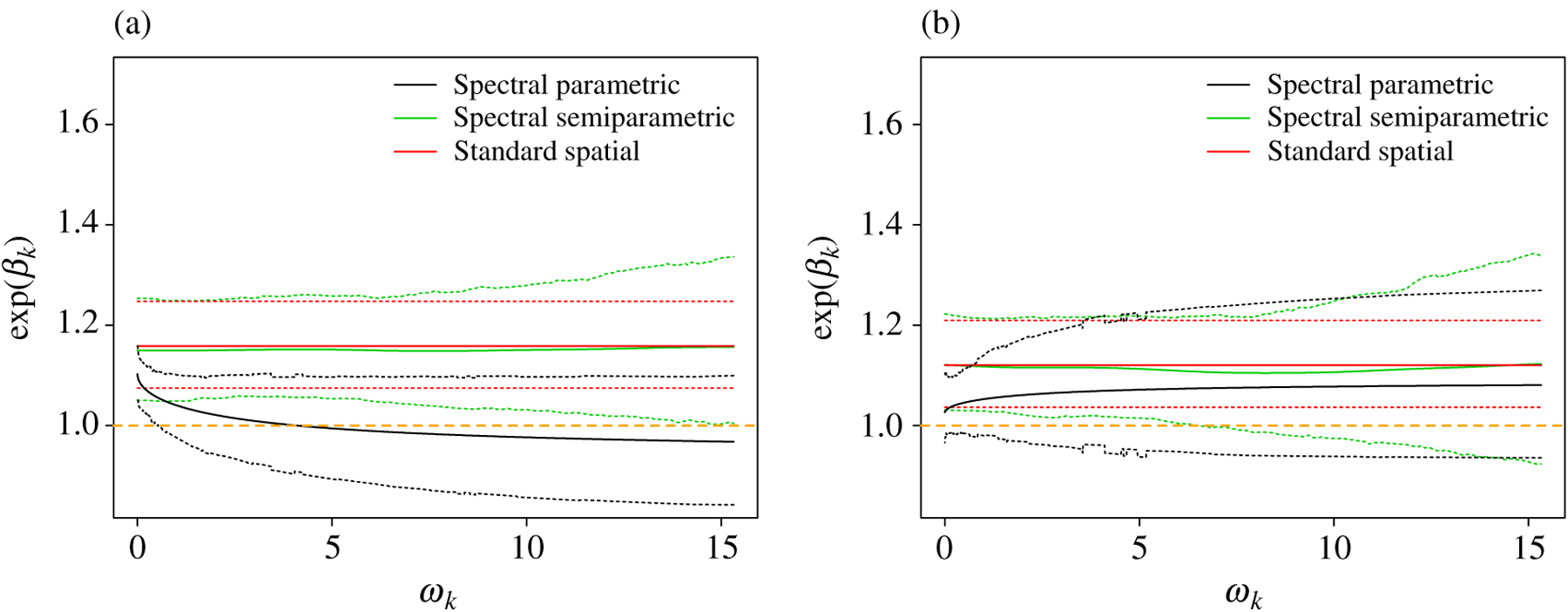
Results for the COVID-19 example: the posterior mean (solid) and 95% credible interval (dashed) of the mortality rate ratio associated with a difference of $1\mu \mathrm{g}/m^3$ of PM_2.5, $\mathrm{e}\mathrm{x}\mathrm{p}\left({\beta }_k\right)$. Results are for (a) all $n=3109$ counties and (b) $n=1977$ counties that reported at least 10 confirmed COVID-19 deaths. The standard spatial approach refers to a regression model including all confounders and a spatial Leroux model for county random effects.

7. Discussion

Our work is the first to study the problem of spatial confounding in the spectral domain and model the coherence between the exposure and the unmeasured spatial confounder. We provide theoretical results that help understand the study in Paciorek (2010), where extensive simulations illustrate the bias obtained under different combinations of spatial scales for $X$ and $Z$. New spectral methods are also proposed to adjust for unmeasured spatial confounding variables, and sufficient conditions are provided to ensure that the exposure effect is identifiable, including the important case without a nugget effect in the treatment and/or response variable. These ideas are developed for continuous and discrete spatial domains, and Gaussian and non-Gaussian data.

We have assumed that $X$ and $Z$ are stationary Gaussian processes in developing our methodology. Such modelling assumptions often work well with weak nonstationarity. With strong nonstationarity under model misspecification, we believe that the semiparametric model is more robust, and that ${\beta }_x$ estimation will be primarily driven by observations from the regions that have variations at smaller spatial scales. We recommend gravitating towards the semiparametric approach. The parametric parsimonious model depends on scale-invariant coherence between the exposure and the unmeasured confounder; it also relies on parsimonious parameterization for estimation of $\alpha \left(\omega \right)$. The semiparametric model depends on the assumption that their coherence tends to zero for large frequencies. While neither of these assumptions are empirically verifiable, we believe that the latter assumption is more reasonable in practice. The semiparametric methods are also easier to implement computationally as the confounding adjustment takes the form of smoothed covariates; it is straightforward to pass these constructed variables into standard spatial computing packages. However, the continuous-space semiparametric model requires numerical approximations to integrals. When the exposure observations are highly spatially irregular, our implementation in § 3.2 can be problematic. In this case, we recommend seeking other numerical approximations to integrals.

References

- Apanasovich TV, Genton MG & Sun Y (2012). A valid Matérn class of cross-covariance functions for multivariate random fields with any number of components. J. Am. Statist. Assoc 107, 180–93. [Google Scholar]
- Chen K, Dai F, Marchiori E & Theodoridis S (2021). Novel compressible adaptive spectral mixture kernels for Gaussian processes with sparse time and phase delay structures. ar Xiv: 1808.00560v8. [Google Scholar]
- Clayton DG, Bernardinellli L & Montomoli C (1993). Spatial correlation in ecological analysis. Int. J. Epidemiol 22, 1193–202. [DOI] [PubMed] [Google Scholar]
- Dupont E, Wood SN & Augustin N (2022). Spatial+: a novel approach to spatial confounding. Biometrics 78, 1279–90. [DOI] [PMC free article] [PubMed] [Google Scholar]
- Eilers PHC & Marx BD (1996). Flexible smoothing with b-splines and penalties. Statist. Sci 11, 89–102. [Google Scholar]
- Faes L, Krohova J, Pernice R, Busacca A & Javorka M (2019). A new frequency domain measure of causality based on partial spectral decomposition of autoregressive processes and its application to cardiovascular interactions. In 2019 41st Ann. Int. Conf. IEEE Eng. Med. Biol. Soc. (EMBC), pp. 4258–61. Piscataway, NJ: IEEE Press. [DOI] [PubMed] [Google Scholar]
- Franco-Villoria M, Ventrucci M & Rue H (2019). A unified view on Bayesian varying coefficient models. Electron. J. Statist 13, 5334–59. [Google Scholar]
- Fuentes M & Reich B (2010). Spectral domain. In Handbook of Spatial Statistics, Gelfand AE, Diggle P, Fuentes M & Guttorp P, eds. Boca Raton, FL: CRC Press, pp. 57–77. [Google Scholar]
- Gelfand AE, Diggle P, Fuentes M & Guttorp P, Ed. (2010). Handbook of Spatial Statistics. Boca Raton, FL: CRC Press. [Google Scholar]
- Gneiting T, Kleiber W & Schlather M (2010). Matérn cross-covariance functions for multivariate random fields. J. Am. Statist. Assoc 105, 1167–77. [Google Scholar]
- Hanks EM, Schliep EM, Hooten MB & Hoeting JA (2015). Restricted spatial regression in practice: geostatistical models, confounding, and robustness under model misspecification. Environmetrics 26, 243–54. [Google Scholar]
- Hodges JS & Reich BJ (2010). Adding spatially-correlated errors can mess up the fixed effect you love. Am. Statistician 64, 325–34. [Google Scholar]
- Hughes J & Haran M (2013). Dimension reduction and alleviation of confounding for spatial generalized linear mixed models. J. R. Statist. Soc. B 75, 139–59. [Google Scholar]
- Jang PA, Loeb A, Davidow M & Wilson AG (2017). Scalable Levy process priors for spectral kernel learning. In Advances in Neural Information Processing Systems, pp. 3943–52. New York: Curran Associates. [Google Scholar]
- Johnson C (2012). Numerical Solution of Partial Differential Equations by the Finite Element Method. New York: Dover Publications. [Google Scholar]
- Keller JP & Szpiro AA (2020). Selecting a scale for spatial confounding adjustment. J. R. Statist. Soc. A 183, 1121–43. [DOI] [PMC free article] [PubMed] [Google Scholar]
- Khan K & Calder CA (2022). Restricted spatial regression methods: implications for inference. J. Am. Statist. Assoc 117, 482–94. [DOI] [PMC free article] [PubMed] [Google Scholar]
- Kleiber W (2017). Coherence for multivariate random fields. Statist. Sinica 27, 1675–97. [Google Scholar]
- Leroux BG, Lei X & Breslow N (2000). Estimation of disease rates in small areas: a new mixed model for spatial dependence. In Statistical Models in Epidemiology, the Environment, and Clinical Trials, Halloran ME & Berry D, eds. New York: Springer, pp. 179–91. [Google Scholar]
- Lindgren F, Rue H & Lindström J (2011). An explicit link between Gaussian fields and Gaussian Markov random fields: the stochastic partial differential equation approach. J. R. Statist. Soc. B 73, 423–98. [Google Scholar]
- Marques I, Kneib T & Klein N (2022). Mitigating spatial confounding by explicitly correlating Gaussian random fields. Environmetrics 33, e2727. [Google Scholar]
- Osama M, Zachariah D & Schön TB (2019). Inferring heterogeneous causal effects in presence of spatial confounding. In Proc. 36th Int. Conf. Mach. Learn., Long Beach, California, vol. 97, Chaudhuri K & Salakhutdinov R, eds. PMLR, pp. 4942–50. [Google Scholar]
- Paciorek CJ (2010). The importance of scale for spatial-confounding bias and precision of spatial regression estimators. Statist. Sci 25, 107–25. [DOI] [PMC free article] [PubMed] [Google Scholar]
- Page GL, Liu Y, He Z & Sun D (2017). Estimation and prediction in the presence of spatial confounding for spatial linear models. Scand. J. Statist 44, 780–97. [Google Scholar]
- Prates MO, Assunção RM & Rodrigues EC (2019). Alleviating spatial confounding for areal data problems by displacing the geographical centroids. Bayesian Anal. 14, 623–47. [Google Scholar]
- Qadir GA & Sun Y (2020). Semiparametric estimation of cross-covariance functions for multivariate random fields. Biometrics 77, 547–60. [DOI] [PubMed] [Google Scholar]
- R Development Core Team (2023). R: A Language and Environment for Statistical Computing. Vienna, Austria: R Foundation for Statistical Computing. ISBN 3-900051-07-0, http://www.R-project.org. [Google Scholar]
- Reich BJ & Fuentes M (2012). Nonparametric Bayesian models for a spatial covariance. Statist. Methodol 9, 265–74. [DOI] [PMC free article] [PubMed] [Google Scholar]
- Reich BJ, Hodges JS & Zadnik V (2006). Effects of residual smoothing on the posterior of the fixed effects in disease-mapping models. Biometrics 62, 1197–206. [DOI] [PubMed] [Google Scholar]
- Reich BJ, Yang S, Guan Y, Giffin AB, Miller MJ & Rappold A (2021). A review of spatial causal inference methods for environmental and epidemiological applications. Int. Statist. Rev 89, 605–34. [DOI] [PMC free article] [PubMed] [Google Scholar]
- Rue H, Martino S & Chopin N (2009). Approximate Bayesian inference for latent Gaussian models by using integrated nested Laplace approximations. J. R. Statist. Soc. B 71, 319–92. [Google Scholar]
- Sandryhaila A & Moura JMF (2013). Discrete signal processing on graphs: graph Fourier transform. In 2013 IEEE Int. Conf. Acoust. Speech Sig. Proces., pp. 6167–70. Piscataway, NJ: IEEE Press. [Google Scholar]
- Schnell P & Papadogeorgou G (2020). Mitigating unobserved spatial confounding when estimating the effect of supermarket access on cardiovascular disease deaths. Ann. Appl. Statist 14, 2069–95. [Google Scholar]
- Spiegelhalter DJ, Best NG, Carlin BP & Van Der Linde A (2002). Bayesian measures of model complexity and fit. J. R. Statist. Soc. B 64, 583–639. [Google Scholar]
- Stokes PA & Purdon PL (2017). A study of problems encountered in Granger causality analysis from a neuroscience perspective. Proc. Nat. Acad. Sci 114, E7063–72. [DOI] [PMC free article] [PubMed] [Google Scholar]
- Thaden H & Kneib T (2018). Structural equation models for dealing with spatial confounding. Am. Statistician 72, 239–52. [Google Scholar]
- Watson GN (1995). A Treatise on the Theory of Bessel Functions. Cambridge: Cambridge University Press. [Google Scholar]
- Wu X, Nethery RC, Sabath BM, Braun D & Dominici F (2020). Air pollution and COVID-19 mortality in the United States: strengths and limitations of an ecological regression analysis. Sci. Adv 6, 1–6. [DOI] [PMC free article] [PubMed] [Google Scholar]
- Zimmerman DL & Hoef JMV (2022). On deconfounding spatial confounding in linear models. Am. Statistician 76, 159–67. [Google Scholar]
Associated Data
This section collects any data citations, data availability statements, or supplementary materials included in this article.