Statistical inference on qualitative differences in the magnitude of an effect

Abstract

Qualitative interactions occur when a treatment effect or measure of association varies in sign by sub-population. Of particular interest in many biomedical settings are absence/presence qualitative interactions, which occur when an effect is present in one sub-population but absent in another. Absence/presence interactions arise in emerging applications in precision medicine, where the objective is to identify a set of predictive biomarkers that have prognostic value for clinical outcomes in some sub-population but not others. They also arise naturally in gene regulatory network inference, where the goal is to identify differences in networks corresponding to diseased and healthy individuals, or to different subtypes of disease; such differences lead to identification of network-based biomarkers for diseases. In this paper, we argue that while the absence/presence hypothesis is important, developing a statistical test for this hypothesis is an intractable problem. To overcome this challenge, we approximate the problem in a novel inference framework. In particular, we propose to make inferences about absence/presence interactions by quantifying the relative difference in effect size, reasoning that when the relative difference is large, an absence/presenceinteractionoccurs.Theproposedmethodologyisillustratedthrougha simulation study as well as an analysis of breast cancer data from the Cancer Genome Atlas.

1 |. INTRODUCTION

An objective of many biomedical studies is to identify and test for interactions, which arise when a measure of effect or association between variables differs by sub-population^1,2,3. Precision medicine and genetic network inference provide examples of areas in which interactions are of interest. For instance, researchers in precision medicine seek to understand how patients’ characteristics are associated with heterogeneity in response to treatment. In omics data analysis, it is of interest to determine how biological networks, which summarize the associations between genes/proteins/etc, depend on phenotype.

Interactions may lack clinical or scientific significance when differences in effect are small. In addition to detecting interactions, it is important to identify which are meaningful. For example, in precision medicine, the most important differences in treatment effect may be those in which some sub-populations of patients benefit from the treatment, while other sub-populations are harmed or unaffected. Additionally, one may want to identify differences among sub-populations in the set of biomarkers that have prognostic value for a health outcome — that is, to determine whether some biomarkers are predictive of the outcome in only a subset of the full population. Genetic network inference provides another example: When comparing sub-population level genetic networks, it may be of primary interest to identify pairs of genes that share an association in some sub-populations but share no association in others, or to identify pairs that have a positive association in one sub-population and a negative association in another. This is known as differential network analysis^4,5.

Such qualitative interactions are the focus of this paper. Qualitative interactions occur when a measure of association differs in sign by sub-population. We consider two types of qualitative interactions: positive/negative interactions — also known in the literature as cross-over interactions⁶ — and absence/presence interactions — sometimes referred to as pure interactions⁷. Positive/negative interactions occur when an effect is positive in one sub-population and negative in another, and absence/presence interactions occur when the effect is present in one population but absent in another.

Our objective is to formally test for qualitative interactions, given independent samples from each sub-population. Testing for positive/negative interactions is well-studied, with several procedures available for identifying positive/negative interactions in a fixed number of sub-populations^{6,8,9,10,11,12}. More recent work has also extended to identifying interactions when there is a large, or possibly infinite, number of sub-groups^{13,14,15,16,17}. In contrast to positive/negative interactions, testing for absence/presence interactions has received little attention. Naïve approaches, to be discussed in Section 2.3, require an untenable minimum signal strength condition — that if an effect is present in any sub-population, it is large enough to be detected with absolute certainty. No approaches exist, to the best of our knowledge, that avoid this assumption.

In this paper, we propose a novel framework for inference about absence/presence interactions in two sample settings. Our proposed methodology allows for well-calibrated hypothesis testing under mild assumptions. We also introduce a numerical summary that measures the strength of absence/presence interactions, while accounting for the uncertainty associated with parameter estimation. Additionally, we describe methods for simultaneous inference about absence/presence and positive/negative interactions. The methodology we introduce provides an effective and flexible inference tool in precision medicine and genetic network analysis, as we illustrate in simulations and an analysis of breast cancer data from The Cancer Genome Atlas (TCGA).

2 |. BACKGROUND

2.1 |. Notation

As we begin to formalize the problem, we first introduce some notation. We consider two sub-populations, labeled by $g\in \{1,2\}$. Let ${\theta }_g\in \mathbb{R}$ denote a measure of association in sub-population $g$. For simplicity, we assume that ${\theta }_g$ is finite. When convenient, we write $\theta =\left({\theta }_1,{\theta }_2\right)$. We can consider various measures of association, such as: correlation coefficients, indicating the strength of linear relationship between two variables of interest; $\mathrm{l}\mathrm{o}\mathrm{g}$ odds ratios, describing the relationship between predictors and a binary outcome; and log hazard ratios, describing the association between predictors and a time-to-event outcome.

We assume that given i.i.d. samples of size $n_1$ and $n_2$ from each sub-population, $\sqrt{n_g}$-consistent and asymptotically normal estimators ${\hat{\theta }}_g$ of ${\theta }_g$ are available, i.e.,

$$\sqrt{n_g}({\hat{\theta }}_g-{\theta }_g){\to }_{d}N\left(0,{\sigma }_g^2\right),$$

with ${\sigma }_g^2>0$ denoting the asymptotic variance. For expositional simplicity, we assume balanced sample sizes $n_1=n_2=n$ (key results are stated more generally in the Appendix). We also assume ${\sigma }_g^2$ is known, though we can instead use a consistent estimate, as is commonly done in practice.

We now formally state the null hypotheses of no positive/negative interactions and no absence/presence interaction, labeled $H_0^{\mathrm{P}/\mathrm{N}}$ and $H_0^{\mathrm{A}/\mathrm{P}}$, respectively:

$$H_0^{\mathrm{P}/\mathrm{N}}:{\theta }_g\ge 0\text{for}g\in \{1,2\}\mathbf{or}{\theta }_g\le 0\text{for}g\in \left\{1,2\right\}$$ (1)

$$H_0^{\mathrm{A}/\mathrm{P}}:{\theta }_g=0\text{for}g\in \{1,2\}\mathbf{or}{\theta }_g\ne 0\text{for}g\in \left\{1,2\right\}$$ (2)

We let ${\mathrm{\Theta }}_0^{\mathrm{P}/\mathrm{N}},{\mathrm{\Theta }}_0^{\mathrm{A}/\mathrm{P}}$ and ${\mathrm{\Theta }}_1^{\mathrm{P}/\mathrm{N}},{\mathrm{\Theta }}_1^{\mathrm{A}/\mathrm{P}}$ denote the corresponding null and alternative regions of the parameter space, depicted in the left and center panels of Figure 1 (Recall that the null region is the set of parameters such that the null hypothesis holds, and the alternative region is the complement of the null region.) The positive/negative null region is the union of the the non-negative and non-positive orthants, and the absence/presence null region is the union of all open orthants and the origin.

Figure 1.

Null and alternative regions of parameter space for positive/negative (left; introduced in Section 2.1), absence/presence (center; introduced in Section 2.1), and relative difference hypotheses (right; introduced in Section 3.1)

2.2 |. Testing Composite Null Hypotheses

Our goal is to use the estimate $\hat{\theta }$ to perform tests of $H_0^{\mathrm{P}/\mathrm{N}}$ and $H_0^{\mathrm{A}/\mathrm{P}}$ such that the size is controlled asymptotically under mild assumptions. Recall that for a null hypothesis $H_0$ with accompanying null region ${\mathrm{\Theta }}_0$, the size of a test is defined as

$$\underset{{\theta }_0\in {\mathrm{\Theta }}_0}{\mathrm{s}\mathrm{u}\mathrm{p}} \mathbb{P}\text{(“Reject}\text{the}\text{null}\text{hypothesis”}\mid \theta ={\theta }_0\text{).}$$

In words, the size is the largest possible type-I error rate that could be achieved under any probability distribution given that $\theta$ belongs to the null region.

Here, we describe our general approach for controlling the size at a pre-specified level $\alpha \in (0,1)$. We first define a test statistic $T$, a map from observable data to a real-valued number, with larger values of $T$ corresponding to more evidence against the null hypothesis. We then calculate the test statistic on the observed data, which we denote by $t$. We write $\mathbb{P}\left(T>t\mid \theta ={\theta }_0\right)$ as the probability of observing a random test statistic at least as large as the observed value $t$, assuming $\theta ={\theta }_0$. We reject the null hypothesis if

$$\rho \left(t\right)\equiv \underset{{\theta }_0\in {\mathrm{\Theta }}_0}{\mathrm{s}\mathrm{u}\mathrm{p}} \mathbb{P}\left(T>t\mid \theta ={\theta }_0\right)<\alpha .$$

One can think of $\mathbb{P}\left(T>t\mid \theta ={\theta }_0\right)$ as the p-value under a specific null distribution $\theta ={\theta }_0$; $\rho \left(t\right)$ is then the largest of all such p-values. We reject $H_0$ when there is sufficient evidence to reject all hypotheses $\theta ={\theta }_0$. We can view $\rho \left(t\right)$ as a generalization of the usual p-value for simple null hypotheses to tests with composite null hypotheses, and we will simply refer to $\rho \left(t\right)$ as “p-value”. Tests of the above form are guaranteed to control the size¹⁸.

2.3 |. Existing Methodology

We now review existing approaches to test for qualitative interactions. We first discuss testing positive/negative interactions before moving to absence/presence interactions.

Gail and Simon⁶ developed the most widely used procedure to test for positive/negative interactions. Though Gail and Simon proposed a general $K$-sample test, we focus on the two-sample problem in this paper. We note that various $K$-sample tests for positive/negative interactions have been proposed^8,10,11, but these procedures are essentially equivalent to the Gail-Simon test in the two-sample setting.

Gail and Simon’s approach is to perform a likelihood ratio test based on the asymptotic sampling distribution of $\hat{\theta }$. The likelihood ratio test rejects $H_0^{\mathrm{P}/\mathrm{N}}$ for large values of

$$-\frac{{\mathrm{s}\mathrm{u}\mathrm{p}}_{\left(a_1,a_2\right)\in {\mathrm{\Theta }}_0^{\mathrm{P}/\mathrm{N}}} {\prod }_{g\in \left\{\mathrm{1,2}\right\}} \varphi \left\{\sqrt{n}{\sigma }_g^{-1}({\hat{\theta }}_g-a_g)\right\}}{{\mathrm{s}\mathrm{u}\mathrm{p}}_{\left(b_1,b_2\right)\in {\mathbb{R}}^2} {\prod }_{g\in \left\{\mathrm{1,2}\right\}} \varphi \left\{\sqrt{n}{\sigma }_g^{-1}({\hat{\theta }}_g-b_g)\right\}},$$

where $\varphi (\cdot )$ is the standard normal density. By performing algebraic manipulations, one can show that the likelihood ratio test equivalently rejects the null for large values of

$$T^{P/N}=\underset{\left(a_1,a_2\right)\in {\mathrm{\Theta }}_0^{P/N}}{\min }\sum _{g\in \left\{1,2\right\}}n{\left\{{\sigma }_g^{-1}({\hat{\theta }}_g-a_g)\right\}}^2.$$

The test statistic $T^{\mathrm{P}/\mathrm{N}}$ can be interpreted as the shortest distance between $\hat{\theta }$ and the null region, where the distance is inversely weighted by the asymptotic variances of the estimates, as illustrated in the left panel of Figure 2

Figure 2.

Geometric interpretation of likelihood ratio statistic for the positive/negative hypothesis (left; introduced in Section 2.3) and relative difference hypotheses (right; introduced in Section 3.2)

Gail and Simon show that the test statistic $T^{\mathrm{P}/\mathrm{N}}$ can be calculated as

$$T^{\mathrm{P}/\mathrm{N}}=\underset{g\in \left\{\mathrm{1,2}\right\}}{\mathrm{m}\mathrm{i}\mathrm{n}} \left\{n{({\hat{\theta }}_g/{\sigma }_g)}^2\right\}\mathbb{1}(\hat{\theta }\in {\mathrm{\Theta }}_1^{\mathrm{P}/\mathrm{N}}),$$

where $1(\cdot )$ denotes the indicator function. Furthermore, one can verify that for all $t>0$, the p-value is easily calculated as

$${\rho }^{\mathrm{P}/\mathrm{N}}(t)=\underset{{\theta }_0\in {\mathrm{\Theta }}_0^{\mathrm{P}/\mathrm{N}}}{\mathrm{s}\mathrm{u}\mathrm{p}} \underset{n\to \mathrm{\infty }}{\mathrm{l}\mathrm{i}\mathrm{m}} \mathbb{P}(T^{\mathrm{P}/\mathrm{N}}>t\mid \theta ={\theta }_0)=\frac{1}{2}\mathbb{P}\left({\chi }_1^2>t\right).$$

The likelihood ratio test is quite intuitive and rejects the null when a positive estimate of association is observed in one population, a negative estimate is observed in another population, and both associations are statistically significant.

Now, we discuss approaches to test for absence/presence interactions. While one might be tempted to perform a likelihood ratio test for absence/presence interactions, the likelihood ratio test fails in the sense that it never can reject the null. To see this, we first recognize that, similar to the positive/negative interaction test, the absence/presence likelihood ratio test would reject for large values of

$$T^{A/P}=\underset{\left(a_1,a_2\right)\in {\mathrm{\Theta }}_0^{A/P}}{min}\sum _{g\in \left\{1,2\right\}}n{\left\{{\sigma }_g^{-1}({\hat{\theta }}_g-a_g)\right\}}^2.$$

Again, the test statistic $T^{\mathrm{A}/\mathrm{P}}$ is the shortest distance between $\hat{\theta }$ and the null region ${\mathrm{\Theta }}_0^{\mathrm{A}/\mathrm{P}}$. However, because the alternative region ${\mathrm{\Theta }}_1^{\mathrm{A}/\mathrm{P}}$ has zero area, $\hat{\theta }$ lies in the null region with probability one. Therefore, the test statistic is always 0, and the likelihood ratio test has no power.

One might alternatively attempt to test the absence/presence null by separately testing the null hypotheses $H_0^g:{\theta }_g=0$ for $g\in \{1,2\}$ and rejecting the absence/presence null when $H_0^g$ is rejected for one $g$ and not rejected for the other. To control the size of a test of this form, which we refer to as the naïve test for the absence/presence null, we need to simultaneously control the type-I error under two scenarios: (1) there is an association in both sub-populations, and (2) there is no association in either population. When there is an association in both populations, a type-I error occurs when we incorrectly fail to reject one of $H_0^g$. When there is no association in either population, we make a type-I error when we incorrectly reject one of $H_0^g$. Thus, controlling the size of the test for $H_0^{\mathrm{A}/\mathrm{P}}$ using this approach requires simultaneous control of the type-I error rate and type-II error rate of tests for $H_0^g$. If the tests for $H_0^g$ are consistent — that is, the type-II error rates tend to zero with sufficiently large samples — this approach is asymptotically valid, as only the type-I error rates for tests of $H_0^g$ need to be controlled. However, with even moderately large samples, we will not be able to correctly reject false $H_0^g$ with absolute certainty unless the true association is strong and hence easy to detect. This would make the test of $H_0^{\mathrm{A}/\mathrm{P}}$ unreliable in the presence of weak signal.

Next, we argue that the naïve test controls the type-I error only if ${\theta }_1,{\theta }_2>o\left(n^{-1/2}\right)$, which is similar to the assumption recently made for differential network connectivity analysis ¹⁹. To see this, we construct a more formal argument. For simplicity, suppose ${\sigma }_1={\sigma }_2=1$. We consider tests of $H_0^g$ of the form

$${\psi }_g=\left\{\begin{array}{ll}\text{Reject;}& \text{if}\sqrt{n}|{\hat{\theta }}_g|>a\\ \text{Accept;}& \text{if}\sqrt{n}|{\hat{\theta }}_g|<a\end{array},\right.$$

where $a$ is a constant that would be selected to control the size. The probability of rejecting the absence/presence null is

$$\mathbb{P}(\text{Reject}{H}_0^{\mathrm{A}/\mathrm{P}})=\mathbb{P}\left({\psi }_1=\text{Reject}\right)\mathbb{P}\left({\psi }_2=\text{Accept}\right)+\mathbb{P}\left({\psi }_1=\text{Accept}\right)\mathbb{P}\left({\psi }_2=\text{Reject}\right).$$

Suppose ${\theta }_1$ and ${\theta }_2$ are guaranteed to be greater than $o\left(n^{-1/2}\right)$ if they are both nonzero. Then, for ${\theta }_1,{\theta }_2\ne 0,\sqrt{n}|{\hat{\theta }}_g|\to \mathrm{\infty }$, and $\mathbb{P}(\text{Reject}{H}_0^{\mathrm{A}/\mathrm{P}})\to 0$. Therefore, to control the size, we are only required to select $\alpha$ so that the type-I error is controlled when ${\theta }_1={\theta }_2=0$; this can be done by taking $a$ as the $(1-\alpha /4)$ quantile of the standard normal distribution. However, if we allow ${\theta }_g<o\left(n^{1/2}\right)$, we can see a drastically inflated type-I error rate. For instance, for a small $ϵ>0$, let ${\theta }_1=n^{-1/2+ϵ}$, ${\theta }_2=n^{-1/2-ϵ}$. This asymptotic regime allows us to approximate the type-1 error rate of this test in settings where the sample size is large relative to the signal strength. Then $\sqrt{n}|{\hat{\theta }}_1|\to \mathrm{\infty }>a$ while $\sqrt{n}|{\hat{\theta }}_2|\to 0<a$, so $\mathbb{P}(\mathrm{R}\mathrm{e}\mathrm{j}\mathrm{e}\mathrm{c}\mathrm{t}{H}_0^{\mathrm{A}/\mathrm{P}})\to 1$. Thus, when small signal is permitted, tests of this form will be asymptotically anti-conservative.

Both approaches discussed above for testing absence/presence interactions — namely, the likelihood ratio test and the naïve test — fail for a similar reason: it is difficult to gather evidence supporting that a measure of association is exactly equal to zero. This is captured by the alternative region having zero area, causing the failure of the first approach. In the second approach, to obtain evidence supporting that an association is zero, we require that $H_{0,g}$ is only accepted when ${\theta }_g=0$; for this, we rely upon a minimum signal strength condition to guarantee that any non-zero association is detected.

3 |. PROPOSED METHODOLOGY

3.1 |. Refinement of Absence/Presence Hypothesis

To mitigate the challenges described in Section 2, we consider a refinement of the absence/presence null hypothesis. The key idea is that in practice, absence/presence interactions can be approximated by considering the settings where an association is at least moderately large in one population and negligible or near zero in the other; or when one association is substantially stronger than the other. This means that we can expand the alternative region to include neighborhoods of zero in a way that the absence/presence interpretation is preserved.

Recall that when there exists an absence/presence interaction, the ratio of the maximum of the absolute value of the ${\theta }_g$ to the minimum is infinite. We cannot test that the ratio is infinite because we will never have evidence to support that the denominator is exactly zero. However, we can test that the ratio is large because we may have evidence to support that the denominator is very small. Motivated by this intuition, we propose to test whether the relative difference between sub-population measures of association is greater than a large pre-specified constant $\kappa >1$. Formally, let ${\theta }_{\mathrm{m}\mathrm{a}\mathrm{x}}={\mathrm{m}\mathrm{a}\mathrm{x}}_g \left|{\theta }_g\right|$ and ${\theta }_{\mathrm{m}\mathrm{i}\mathrm{n}}={\mathrm{m}\mathrm{i}\mathrm{n}}_g \left|{\theta }_g\right|$. We define the new relative difference null hypothesis $H_0^{\kappa }$ as

$$H_0^{\kappa }:{\theta }_{\mathrm{m}\mathrm{a}\mathrm{x}}/{\theta }_{\mathrm{m}\mathrm{i}\mathrm{n}}\le \kappa \text{or}{\theta }_{\mathrm{m}\mathrm{a}\mathrm{x}}={\theta }_{\mathrm{m}\mathrm{i}\mathrm{n}}=0.$$

Equivalently,

$$H_0^{\kappa }:{\theta }_{\mathrm{m}\mathrm{a}\mathrm{x}}-\kappa {\theta }_{\mathrm{m}\mathrm{i}\mathrm{n}}\le 0.$$ (3)

The null region ${\mathrm{\Theta }}_0^{\kappa }$, illustrated in the right panel of Figure 1, is the union of four linear subspaces — each residing in a separate orthant of ${\mathbb{R}}^2$; the boundary of each subspace is the union of the spans of vectors with absolute direction $(\kappa ,1{)}^{\prime }$ and $(1,\kappa {)}^{\prime }$.

The relative difference null region can be viewed as a relaxation of the absence/presence null. For a large choice of $\kappa$, the original and refined null hypotheses have a similar interpretation: the greater measure of association is substantially larger than the lesser. However, the hypotheses may not coincide for any value of $\kappa$ as the relative difference hypothesis can hold if ${\theta }_{\mathrm{m}\mathrm{a}\mathrm{x}}$ is non-zero while ${\theta }_{\mathrm{m}\mathrm{i}\mathrm{n}}$ is non-zero but small. It is nonetheless appealing that $H_0^{\kappa }$ has a reasonable interpretation for any choice of $\kappa$; that is, the multiplicative difference in strength of association is no larger than $\kappa$.

To motivate defining the refined null hypothesis in terms of relative differences rather than absolute differences, we argue that testing for relative differences has at least the following benefits. First, relative differences are unitless, so the relative difference null is compatible with unitless measures of association such as the Pearson correlation coefficient, which are often preferred in the analysis of biological data. Second, it is possible that in some contexts, $\kappa$ could be selected without prior knowledge on the range of strength of association. For instance, in studies of differential gene expression in two groups, it is common for investigators to focus on identifying genes for which the relative difference in the mean expression level exceeds a user-specified threshold. The threshold is chosen to be scientifically meaningful, based on the investigator’s own discretion^20,21. When the goal is identifying pairs of genes for which the correlation between gene expression levels differs by group, an investigator could similarly select a scientifically meaningful threshold for the relative difference in correlation at their own discretion.

Of course, the relative difference null hypothesis depends on the choice of $\kappa$. For small values of $\kappa$, the relative difference null may be too dissimilar from the absence/presence null to retain its interpretation; for large $\kappa$, the alternative region becomes very small, and the hypothesis may be overly conservative. In settings where there is a scientifically meaningful threshold for the relative difference in effect size, $\kappa$ can be specified a priori based on its interpretation, often at the investigator’s discretion. In the following subsections, we first construct a test of the relative difference null hypothesis for a pre-specified $\kappa$. We then describe an approach to identify the set of $\kappa$ values for which the test rejects the null hypothesis. This method can be useful when there is no clear scientifically meaningful threshold for the relative difference in effects.

3.2 |. Likelihood Ratio Test for Relative Difference Hypothesis

We next develop a testing procedure for the new relative difference null hypothesis. The relative difference null region, unlike the absence/presence null region, has a non-zero area, so a likelihood ratio test will not fail in the same manner as the likelihood ratio test for the absence/presence hypothesis. Similar to the previously discussed examples, the likelihood ratio test statistic is

$$T^{\kappa }=\underset{\left(a_1,a_2\right)\in {\mathrm{\Theta }}_0^{\kappa }}{\mathrm{m}\mathrm{i}\mathrm{n}} \sum _{g\in \left\{\mathrm{1,2}\right\}} n{\left\{{\sigma }_g^{-1}({\hat{\theta }}_g-a_g)\right\}}^2,$$

and can be interpreted as the shortest (weighted) distance between $\hat{\theta }$ and the null region ${\mathrm{\Theta }}_0^{\kappa }$, as depicted in the right panel of Figure 2 Clearly, the test statistic is zero whenever $\hat{\theta }$ lies in the null region. Otherwise, $T^{\kappa }$ is the shortest distance between $\hat{\theta }$ and the closest of the four linear subspaces that define ${\mathrm{\Theta }}_0^{\kappa }$. The test statistic can be calculated as the distance between ${({\hat{\theta }}_{\text{max}},{\hat{\theta }}_{\text{min}})}^{\prime }$ and its projection onto the span of the vector $(\kappa ,1{)}^{\prime }$.

The likelihood ratio test statistic is straightforward to calculate. Let ${\hat{\theta }}_{\mathrm{m}\mathrm{a}\mathrm{x}}={\mathrm{m}\mathrm{a}\mathrm{x}}_g |{\hat{\theta }}_g|$ and ${\hat{\theta }}_{\text{min}}={\mathrm{m}\mathrm{i}\mathrm{n}}_g |{\hat{\theta }}_g|$ be the strongest and weakest estimated absolute association, respectively. In the following lemma, we state that $T^{\kappa }$ is equal to the difference between ${\hat{\theta }}_{\text{max}}$ and $\kappa {\hat{\theta }}_{\text{min}}$ divided by a normalizing constant. Thus, the test statistic can be viewed as a plug-in of $\hat{\theta }$ into (3) with an additional normalizing constant. This test statistic closely resembles the test statistic proposed by Fieller²² to conduct inference about ratios of means.

Lemma 1.

The likelihood ratio test statistic $T^{\kappa }$ can be written as

$$T^{\kappa }=\frac{{\hat{\theta }}_{\mathrm{m}\mathrm{a}\mathrm{x}}-\kappa {\hat{\theta }}_{\mathrm{m}\mathrm{i}\mathrm{n}}}{\sqrt{{\hat{\tau }}_{\mathrm{m}\mathrm{a}\mathrm{x}}+{\kappa }^2{\hat{\tau }}_{\mathrm{m}\mathrm{i}\mathrm{n}}}},$$

where ${\hat{\tau }}_{\mathrm{m}\mathrm{a}\mathrm{x}}=n^{-1}{\sigma }_1^2\mathbb{1}(|{\hat{\theta }}_1|={\hat{\theta }}_{\mathrm{m}\mathrm{a}\mathrm{x}})+n^{-1}{\sigma }_2^2\mathbb{1}(|{\hat{\theta }}_2|={\hat{\theta }}_{\mathrm{m}\mathrm{a}\mathrm{x}})$, and ${\hat{\tau }}_{\mathrm{m}\mathrm{i}\mathrm{n}}=n^{-1}{\sigma }_1^2\mathbb{1}(|{\hat{\theta }}_1|={\hat{\theta }}_{\text{min}})+n^{-1}{\sigma }_2^2\mathbb{1}(|{\hat{\theta }}_2|={\hat{\theta }}_{\text{min}})$.

We now discuss how to obtain a p-value for the relative difference hypothesis. First, we obtain an observed test statistic $t$, a realization of $T^{\kappa }$ calculated from the data. Following the approach described in Section 2.2, we define the p-value as ${\rho }^{\kappa }\left(t\right)$, the largest of all asymptotic tail probabilities ${\mathrm{l}\mathrm{i}\mathrm{m}}_{n\to \mathrm{\infty }} \mathbb{P}\left(T^{\kappa }>t\mid \theta ={\theta }_0\right)$ such that ${\theta }_0$ belongs to the null region. To determine the maximum tail probability, we characterize the limiting distribution of $T^{\kappa }$ assuming $\theta ={\theta }_0$ for all ${\theta }_0$ in the null region.

Though the null region contains an infinite number of values, $T^{\kappa }$ can only attain one of three limiting distributions corresponding to the following three cases:

1. The true association is in the interior of the null region, i.e., ${\theta }_{\mathrm{m}\mathrm{a}\mathrm{x}}-\kappa {\theta }_{\mathrm{m}\mathrm{i}\mathrm{n}}<0$.

2. The true association is on the boundary of the null region, but both associations are non-zero, i.e., ${\theta }_{\mathrm{m}\mathrm{a}\mathrm{x}}=\kappa {\theta }_{\mathrm{m}\mathrm{i}\mathrm{n}}>0$.

3. The true association is zero in both sub-populations, i.e., ${\theta }_1={\theta }_2=0$.

In Proposition 1, we describe the asymptotic behavior of $T^{\kappa }$ for cases 1 and 2 above. We provide here some intuition for the result and reserve a formal argument for the Appendix. In case 1, it is easy to argue that because $\hat{\theta }$ is consistent, $T^{\kappa }$ is a negative number with probability tending to one, and therefore never provides evidence against the null. In case 2, $T^{\kappa }$ asymptotically follows a standard normal distribution. To see this, we note that because both associations are non-zero, consistency and asymptotic normality of $\hat{\theta }$ imply that, for large $n$, the sign of the estimators and the ranking of their magnitudes are deterministic. That the signs are asymptotically deterministic implies that $|\hat{\theta }|$ is asymptotically normal (speaking loosely, $|{\hat{\theta }}_g|\to \mathrm{s}\mathrm{i}\mathrm{g}\mathrm{n}\left({\theta }_g\right){\hat{\theta }}_g$); that ranking is asymptotically deterministic implies that ${\hat{\theta }}_{\mathrm{m}\mathrm{a}\mathrm{x}}$ and ${\hat{\theta }}_{\text{min}}$ are asymptotically independent. Therefore, taking the difference between ${\hat{\theta }}_{\text{max}}$ and ${\hat{\theta }}_{\text{min}}$, suitably standardized, is asymptotically equivalent to taking a difference between two independent normal random variables with equal means. Dividing by the asymptotic variances gives the claimed result.

Proposition 1.

In the interior of the null region, i.e., when ${\theta }_{\mathrm{m}\mathrm{a}\mathrm{x}}-\kappa {\theta }_{\mathrm{m}\mathrm{i}\mathrm{n}}<0$, $T^{\kappa }$ converges in distribution to $-\mathrm{\infty }$. At all nonzero boundary points of the null region, i.e., when ${\theta }_{\mathrm{m}\mathrm{a}\mathrm{x}}=\kappa {\theta }_{\mathrm{m}\mathrm{i}\mathrm{n}}>0$, $T^{\kappa }$ converges in distribution to a standard normal random variable.

In case 3, when both associations are zero, the asymptotic distribution of the test statistic is more complicated. More specifically, ${\theta }_g=0$ implies that, asymptotically, $|{\hat{\theta }}_g|$ follows a half-normal distribution instead of a normal distribution. Moreover, the ranking of $|{\hat{\theta }}_1|$ and $|{\hat{\theta }}_2|$ remains random in the limit. This gives rise to a non-standard limiting distribution. In particular, unlike cases 1 and 2, the limiting distribution depends on the asymptotic variances of the sub-population estimates (and also the ratio of the sample sizes in the unbalanced case). We are nonetheless able to derive an analytic expression for the distribution function, stated in Proposition 2. We reserve this statement for the Appendix, as the expression is cumbersome.

By Propositions 1 and 2, we can calculate the p-value as the maximum of the tail probabilities in cases 2 and 3. That is,

$${\rho }^{\kappa }\left(t\right)=\mathrm{m}\mathrm{a}\mathrm{x}\left\{1-\mathrm{\Phi }\left(t\right),1-F^{\kappa }\left(t\right)\right\},$$ (4)

where $\mathrm{\Phi }(\cdot )$ denotes the standard normal distribution function, and $F^{\kappa }(\cdot )\equiv {\mathrm{l}\mathrm{i}\mathrm{m}}_{n\to \mathrm{\infty }} \mathbb{P}\left(T^{\kappa }<t\mid \theta ={\theta }_0\right)$ is the limiting distribution function for the test statistic when $\theta =0$. Though the limiting distribution under $\theta =0$ is non-standard, tail probabilities can be calculated easily, as we show in the Appendix (Remark 1). The p-value is therefore simple to calculate.

We have derived an analytic approximation for the power of the likelihood ratio test. In Proposition 2, we more generally characterize the limiting distribution of the test statistic under hypotheses of the form $\left({\theta }_1,{\theta }_2\right)=n^{-1/2}\left(c_1,c_2\right)$. The local asymptotic power of the proposed test at the level $\alpha$ is available by considering ${\beta }_{\alpha }^{\kappa }\left(c_1,c_2\right)\equiv {\mathrm{l}\mathrm{i}\mathrm{m}}_{n\to \mathrm{\infty }} \mathbb{P}\left(T^{\kappa }>t_{1-\alpha }^{\mathrm{*}}\mid \theta =n^{-1/2}\left(c_1,c_2\right)\right)$, where we define $t_{1-\alpha }^{\mathrm{*}}$ as the maximum of the $1-\alpha$ quantiles of the limiting distribution of $T^{\kappa }$ under scenarios 2 and 3 described above. An analytic finite-sample approximation of the power can be calculated as ${\beta }_{\alpha }^{\kappa }\left(n^{1/2}{\theta }_1,n^{1/2}{\theta }_2\right)$.

A contour plot of the local asymptotic power is given in Figure 3 for both equal and unequal variances of the estimators. We observe that the likelihood ratio test has low power when the strongest effect max $\left\{\left|c_1\right|,\left|c_2\right|\right\}$ is small, and power improves considerably when the strongest effect grows. Additionally, we find that in the presence of unequal variance, the test has greater power when the weakest effect is estimated with higher precision than the strongest effect.

Figure 3.

Contour plots of the local asymptotic power of the relative difference likelihood ratio test with $\kappa =2$ and $\alpha =.05$. Bold lines represent the boundary of the null region. Settings of equal and unequal asymptotic variance of estimators are shown.

3.3 |. Quantifying Relative Difference in Effect by Inverting Likelihood Ratio Test

In some applications there may not be a clear scientifically meaningful threshold for the relative difference in effect size. In such settings, investigators may be disinclined to test the relative difference null for a single fixed choice of $\kappa$, as the choice can be somewhat arbitrary. It may be preferable to instead provide a more informative summary describing the relative difference in effect size.

We propose to summarize the relative difference in effect size by reporting the set of $\kappa$ for which we would reject the relative difference null. We define

$${\kappa }_{\mathrm{m}\mathrm{a}\mathrm{x}}^{\alpha }\equiv \mathrm{s}\mathrm{u}\mathrm{p}\left\{\kappa :\kappa >1,{\rho }^{\kappa }\left(t\right)<\alpha \right\}$$

as the largest $\kappa >1$ such that the likelihood ratio test rejects the null hypothesis at the $\alpha$ level. When the likelihood ratio test fails to reject for all $\kappa >1$, we will use the convention ${\kappa }_{\mathrm{m}\mathrm{a}\mathrm{x}}^{\alpha }=1$. Since $T^{\kappa }$ is negative for $\kappa >{\hat{\theta }}_{\mathrm{m}\mathrm{a}\mathrm{x}}/{\hat{\theta }}_{\text{min}}$ and since we only reject the relative difference null for large positive values of $T^{\kappa }$, ${\kappa }_{\mathrm{m}\mathrm{a}\mathrm{x}}^{\alpha }$ is bounded above by ${\hat{\theta }}_{\mathrm{m}\mathrm{a}\mathrm{x}}/{\hat{\theta }}_{\mathrm{m}\mathrm{i}\mathrm{n}}$.

Because the likelihood ratio test controls the type-I error at the level $\alpha$, if ${\theta }_{\mathrm{m}\mathrm{a}\mathrm{x}}={\theta }_{\mathrm{m}\mathrm{i}\mathrm{n}}$, then with probability at least $1-\alpha ,{\kappa }_{\mathrm{m}\mathrm{a}\mathrm{x}}^{\alpha }=1$. Moreover, if ${\theta }_{\mathrm{m}\mathrm{a}\mathrm{x}}/{\theta }_{\mathrm{m}\mathrm{i}\mathrm{n}}>1$, ${\kappa }_{\mathrm{m}\mathrm{a}\mathrm{x}}^{\alpha }$ is bounded above by ${\theta }_{\mathrm{m}\mathrm{a}\mathrm{x}}/{\theta }_{\mathrm{m}\mathrm{i}\mathrm{n}}$ with probability at least $1-\alpha$. Thus, ${\kappa }_{\mathrm{m}\mathrm{a}\mathrm{x}}^{\alpha }$ provides a probabilistic lower bound for the relative difference in effect size. That is,

$$\underset{n\to \mathrm{\infty }}{\mathrm{l}\mathrm{i}\mathrm{m}} \mathbb{P}\left({\kappa }_{\mathrm{m}\mathrm{a}\mathrm{x}}^{\alpha }\le {\theta }_{\mathrm{m}\mathrm{a}\mathrm{x}}/{\theta }_{\mathrm{m}\mathrm{i}\mathrm{n}}\right)\ge 1-\alpha .$$

Moreover, for any $\kappa <{\theta }_{\mathrm{m}\mathrm{a}\mathrm{x}}/{\theta }_{\text{min}}$, the relative difference test will reject the null hypothesis that ${\theta }_{\mathrm{m}\mathrm{a}\mathrm{x}}\le \kappa {\theta }_{\text{min}}$ with probability tending to one. Therefore, in the limit of large $n$, ${\kappa }_{\mathrm{m}\mathrm{a}\mathrm{x}}^{\alpha }$ should approach but not exceed the true relative difference in effect size. We discuss the calculation of ${\kappa }_{\mathrm{m}\mathrm{a}\mathrm{x}}^{\alpha }$ in the Appendix.

Larger values of ${\kappa }_{\mathrm{m}\mathrm{a}\mathrm{x}}^{\alpha }$ indicate that the relative difference in effect ${\theta }_{\mathrm{m}\mathrm{a}\mathrm{x}}/{\theta }_{\mathrm{m}\mathrm{i}\mathrm{n}}$ is large and provide greater evidence to support the occurrence of an absence/presence interaction. However, we emphasize that no value of ${\kappa }_{\mathrm{m}\mathrm{a}\mathrm{x}}^{\alpha }$ will be large enough to guarantee that an absence presence interaction has truly occurred. While we argue that ${\kappa }_{\mathrm{m}\mathrm{a}\mathrm{x}}^{\alpha }$ is an informative and intuitive summary, we caution investigators against misinterpreting it.

3.4 |. Simultaneous Test for Qualitative Interactions

When it is of interest to identify both absence/presence and positive/negative qualitative interactions, it may be desirable to test for both simultaneously. In this section, we construct an omnibus test that achieves control of the size asymptotically.

We define the omnibus qualitative interaction null hypothesis as

$$H_0^{\mathrm{P}/\mathrm{N},\kappa }:\text{Both}{H}_0^{\mathrm{P}/\mathrm{N}}\text{and}{H}_0^{\kappa }\text{hold.}$$

The null region ${\mathrm{\Theta }}_0^{\mathrm{P}/\mathrm{N},\kappa }$ is the intersection of the positive/negative and relative difference null regions, as depicted in Figure 4 We observe that as $\kappa \to \mathrm{\infty }$, the omnibus null and alternative regions tend to the positive/negative null and alternative regions.

Figure 4.

(Left) Null and alternative region for omnibus qualitative interaction hypothesis. (Right) Geometric interpretation of likelihood ratio statistic for the omnibus qualitative interaction hypothesis.

To construct the likelihood ratio test, we proceed using similar arguments to those presented in Section 3.2. The likelihood ratio statistic $T^{\mathrm{P}/\mathrm{N},\kappa }$ is the distance between the estimate $\hat{\theta }$ and its projection onto the null region ${\mathrm{\Theta }}_0^{\mathrm{P}/\mathrm{N},\kappa }$, inversely weighted by the asymptotic variance of $\hat{\theta }$. A simple expression for $T^{\mathrm{P}/\mathrm{N},\kappa }$ is given in Lemma 2.

Lemma 2.

The likelihood ratio statistic $T^{\mathrm{P}/\mathrm{N},\kappa }$ can be written as

$$T^{\mathrm{P}/\mathrm{N},\kappa }=\mathrm{m}\mathrm{i}\mathrm{n}\left\{\frac{{({\hat{\theta }}_1-\kappa {\hat{\theta }}_2)}^2}{n^{-1}\left({\sigma }_1^2+{\kappa }^2{\sigma }_2^2\right)},\frac{{(\kappa {\hat{\theta }}_1-{\hat{\theta }}_2)}^2}{n^{-1}({\kappa }^2{\sigma }_1^2+{\sigma }_2^2)}\right\}\mathbb{1}\left(\hat{\theta }\in {\mathrm{\Theta }}_1^{\mathrm{P}/\mathrm{N},\kappa }\right).$$

Unsurprisingly, the likelihood ratio statistic for the omnibus test approaches the likelihood ratio statistic for the Gail-Simon likelihood ratio statistic for positive/negative interactions in the limit of large $\kappa$. The tests will, therefore, be nearly identical for sufficiently large $\kappa$.

To characterize the asymptotic behavior of the omnibus test statistic at each location under the null, we use similar arguments to those in the previous section. If $\theta$ belongs to the interior of the null region, $T^{\mathrm{P}/\mathrm{N},\kappa }$ converges in probability to zero. If $\theta$ belongs to the boundary of the null region and is non-zero, $T^{\mathrm{P}/\mathrm{N},\kappa }$ converges weakly to a uniform mixture of zero and the chi-squared distribution with one degree of freedom. If $\theta$ is zero, the limiting distribution of $T^{\mathrm{P}/\mathrm{N},\kappa }$ is non-standard, though it can be characterized nonetheless. Formal statements of asymptotic properties of $T^{\mathrm{P}/\mathrm{N},\kappa }$ are given in Propositions 3 and Remark 2 (the statement of Remark 2 is also cumbersome, and is reserved for the Appendix).

We have derived an analytic approximation for the power of the likelihood ratio test. In Proposition 4 in the Appendix, we more generally characterize the limiting distribution of the test statistic under hypotheses of the form $\left({\theta }_1,{\theta }_2\right)=n^{-1/2}\left(c_1,c_2\right)$, and in Remark 3, also in the Appendix, we describe how this result can be applied to calculate the local asymptotic power of the proposed test.

Proposition 3.

If $\theta$ belongs to the interior of the null region ${\mathrm{\Theta }}_0^{P/N,\kappa }$, $T^{\mathrm{P}/\mathrm{N},\kappa }$ converges in distribution to zero. If $\theta$ is on the boundary of the null region, but $\theta \ne 0$, $\mathbb{P}(T^{\mathrm{P}/\mathrm{N},\kappa }>t)\to \frac{1}{2}P\left({\chi }_1^2>t\right)$ as $n\to \mathrm{\infty }$.

Calculating the p-value for the omnibus test is no more difficult than calculating the p-value for the absence/presence test. Defining $F^{\mathrm{P}/\mathrm{N},\kappa }(t)\equiv {\mathrm{l}\mathrm{i}\mathrm{m}}_{n\to \mathrm{\infty }} \mathbb{P}(T^{\mathrm{P}/\mathrm{N}}<t\mid \theta =0)$, the p-value can be calculated as

$${\rho }^{\mathrm{P}/\mathrm{N},\kappa }(t)=\mathrm{m}\mathrm{a}\mathrm{x}\{\mathbb{P}\left({\chi }_1^2>t\right),1-F^{\mathrm{P}/\mathrm{N},\kappa }(t)\}$$ (5)

where $t$ is the value of the test statistic $T^{\mathrm{P}/\mathrm{N},\kappa }$ calculated on the observed data.

4 |. SIMULATION STUDY

In a Monte Carlo simulation study, we examine how type-I error rate and statistical power of the likelihood ratio tests for the relative difference in effect are affected by signal strength, sample size, and choice of $\kappa$. Additionally, we examine how ${\kappa }_{\mathrm{m}\mathrm{a}\mathrm{x}}^{\alpha }$ depends on the true sub-population effects and the sample size.

We generate random observations $\left(Y_g,X_g\right)$ in sub-population $g$ under the linear model:

$$Y_g={\theta }_g{X}_g+ϵ;X_g~N(0,1);ϵ~N(0,1).$$

Here, $X_g$ is the predictor of interest, $Y_g$ is the response, and $ϵ$ is white noise. The measure of association in which we are interested is the regression coefficient ${\theta }_g$. We fix ${\theta }_1=1$ and consider ${\theta }_2\in \{-1,-.95,-.9,\dots ,.95,1\}$. A total of 1000 synthetic data sets are randomly generated for each ${\theta }_2$ and $n\in \{50,100,200,400,800,1600\}$.

For each synthetic data set, we perform the relative difference likelihood ratio test and the omnibus test with $\kappa \in \{1.5,2,4,8\}$, and use a significance level of $\alpha =.05$. We additionally calculate ${\kappa }_{\mathrm{m}\mathrm{a}\mathrm{x}}^{\alpha }$ with $\alpha =.05$. Parameter estimation is performed with ordinary least squares, and model-based estimates of the standard error are used. We compare the likelihood ratio test with the naïve test for absence/presence interactions described in Section 2.3, which rejects the null when there is evidence for the existence of an effect in one population but insufficient evidence in the other population. We also compare with a test for quantitative interactions, which rejects the null when there is evidence that ${\theta }_1$ and ${\theta }_2$ are unequal.

In Figure 5, we plot Monte Carlo estimates of the rejection probabilities for the relative difference likelihood ratio test, the naïve test, and the test for quantitative interactions over the range of ${\theta }_2$. We see that the relative difference likelihood ratio test achieves control of size for all choices of $\kappa$ and all sample sizes. Power is largest when $\left|{\theta }_2\right|$ is near zero and is lower for larger values of $\kappa$, as expected, because larger values of $\kappa$ correspond to a larger null region. With $\kappa =8$, the likelihood ratio test has almost zero power when the sample size is small, though we see an improvement in large sample settings.

Figure 5.

Monte Carlo estimate of the rejection probability of the relative difference likelihood ratio test and the naïve test. The white vertical line at ${\theta }_2=0$ corresponds to the single point at which the absence/presence hypothesis does not hold. The solid pink line denotes the specified size $\alpha =.05$

The naïve test of the absence/presence hypothesis exhibits poor type-1 error control. Because the absence/presence does not hold only when ${\theta }_2=0$, a well-calibrated test would reject the null with probability no greater than $\alpha$ for any other value of ${\theta }_2$. However, we can see that the type- 1 error rate of the naïve test is greatly inflated when ${\theta }_2$ resides within a neighborhood of zero, and this is especially true in a small sample setting. Due to the test’s poor calibration, it is difficult to glean any meaningful information from a decision to reject the null hypothesis. While the relative difference test can also have a high rejection probability when ${\theta }_2$ is in a neighborhood of zero, it is more easily interpretable: because this test is well-calibrated, we are able to understand what a decision to reject the null implies about the relationship between ${\theta }_1$ and ${\theta }_2$.

Figure 6 shows the estimated rejection probabilities of the omnibus test for varying ${\theta }_2$. Control of size is achieved in both large and small samples, as expected. For this test, power increases as ${\theta }_2$ tends to −1, and as expected, power decreases with increasing $\kappa$.

Figure 6.

Monte Carlo estimate of the rejection probability of the omnibus test for qualitative interactions. The solid pink line denotes the specified size $\alpha =.05$

In Figure 7. we plot the $\alpha ,$ 0.5, and $(1-\alpha )$ quantiles of ${\kappa }_{\mathrm{m}\mathrm{a}\mathrm{x}}^{\alpha }$ values from 1000 synthetic data sets for each ${\theta }_2$. As we would expect, for any fixed ${\theta }_2$, at least $100(1-\alpha )\mathrm{\%}$ of the ${\kappa }_{\mathrm{m}\mathrm{a}\mathrm{x}}^{\alpha }$ fall below $\left|{\theta }_1\right|/\left|{\theta }_2\right|$. In addition, the $(1-\alpha )$ quantile of the distribution ${\kappa }_{\mathrm{m}\mathrm{a}\mathrm{x}}^{\alpha }$ approaches $\left|{\theta }_1\right|/\left|{\theta }_2\right|$ as sample size increases. However, when the sample size is small, ${\kappa }_{\mathrm{m}\mathrm{a}\mathrm{x}}^{\alpha }$ tends to be much smaller than the relative difference in effect size. This suggests that ${\kappa }_{\mathrm{m}\mathrm{a}\mathrm{x}}^{\alpha }$ is a loose lower bound for the relative difference in effect in a small sample setting, but the bound becomes progressively tighter as the sample size grows.

Figure 7.

Distribution of ${\kappa }_{\mathrm{m}\mathrm{a}\mathrm{x}}^{\alpha }$ calculated on synthetic data. The .05, .50, and .95 quantiles are represented by the dashed blue and solid black curves. The grey curve represents $\left|{\theta }_1\right|/\left|{\theta }_2\right|$, the value ${\kappa }_{\mathrm{m}\mathrm{a}\mathrm{x}}^{\alpha }$ is expected to approach for a given ${\theta }_2$.

5 |. DATA EXAMPLE

In this example, we investigate genetic differences in breast cancer sub-types. Classification of breast cancer based on expression of estrogen receptor (ER) is known to be associated with clinical outcomes. Approximately 70% of breast cancers are estrogen receptor positive (ER+) cancers, meaning that estrogen causes cancer cells to grow²³; breast cancers are otherwise estrogen receptor negative (ER−). Patients with ER+ breast cancer tend to experience better clinical outcomes than ER− patients²⁴.

We conduct an analysis using publicly available data from The Cancer Genome Atlas (TCGA)²⁵. We use clinical data and gene expression data from a total of 806 ER+ patients and 237 ER− patients.

We first investigate the differences between the genetic networks in ER+ and ER− breast cancers. Both ER+ and ER− breast cancer are expected to have similar pathways, but identifying differences between them may be key to understanding the underlying disease mechanisms. We then conduct an analysis to assess whether any genes in a set known to be associated with breast cancer are strongly prognostic of disease outcomes in only one of the estrogen receptor groups.

5.1 |. Differential Network Analysis

Our objective is to determine whether there are any pairs of genes that are much more strongly associated in one estrogen receptor group than the other. We consider the set of $p=145$ genes in the Kyoto Encyclopedia of Genes and Genomes (KEGG)²⁶ breast cancer pathway and measure the association between gene expression levels using the Pearson correlation.

We test the relative difference null hypothesis for each pair of genes with $\kappa \in \{2,2.5,3\}$ and provide the resulting p-values in Table 1. In Figure 8, we display the pairs of genes that are statistically significant at the $\alpha =.05$ level with $\kappa =2$ after a Bonferroni adjustment. Each of the genes progesterone (PGR), insulin-like growth factor 1 (IGF1R), and estrogen receptor 1 (ESR1) have multiple differential connections; each belongs to at least two pairs such that the association is twice as strong in the ER+ population than in the ER− population. These genes have been shown in the literature to be associated with sub-type and prognosis^27,28,29.

Table 1.

Bonferroni-adjusted p-values for pairs of genes that genes for which we reject the relative difference hypothesis with κ = 2, κ = 2.5, or κ = 3.

Gene Pair	κ =2	κ = 2.5	κ =3
(IGF1R, AKT3)	0.034	1	1
(IGF1R, FGF1)	0.0011	0.16	1
(KIT, EGFR)	0.0069	1	1
(PGR, FGF7)	0.00034	0.17	1
(PGR, DLL1)	0.014	0.5	1
(PGR, NOTCH4)	6.5e-07	0.00054	0.04
(FZD4, PGR)	8.8e-08	0.00013	0.013
(FGF18, FGF10)	0.017	0.74	1
(E2F1,ESR1)	3.2e-07	0.001	0.13
(E2F2, ESR1)	0.00094	0.11	1

Figure 8.

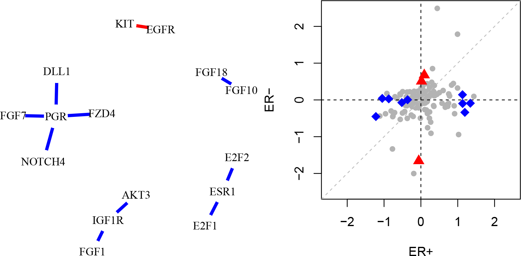
(Left) Pairs of genes in the KEGG breast cancer pathway for which we reject the relative difference hypothesis with $\kappa =2$. Blue edges indicate associations that are stronger in the ER+ group, and red edges indicate associations that are stronger in the ER− group. (Right) Log hazard ratios for KEGG genes in ER+ and ER− groups. The gray dashed line represents the 45-degree line. Blue diamonds and red triangles indicate genes for which ${\kappa }_{\mathrm{m}\mathrm{a}\mathrm{x}}^{\alpha }>1$ with $\alpha =.10$, where the largest log hazard ratio is in the ER+ group and ER− group, respectively.

5.2 |. Prognostic Value of Biomarkers

The goal of this analysis is to assess whether any of the KEGG genes have a stronger association with time to death in one estrogen receptor group than in the other. For each gene, we fit a univariate Cox proportional-hazards model with time to death as the outcome in both of the estrogen receptor groups separately; we measure association using the log hazard ratio. A total of 64 deaths occurred in the ER+ group, and 33 deaths occurred the ER− group. We calculate ${\kappa }_{\mathrm{m}\mathrm{a}\mathrm{x}}^{\alpha }$ for $\alpha$ equal to .1, .05, .025, and .01, for each gene.

In Figure 8, we compare the log hazard ratios of the ER+ and ER− groups in a scatterplot. Though the log hazard ratios for most genes are similar between subgroups, there are twelve genes with ${\kappa }_{\mathrm{m}\mathrm{a}\mathrm{x}}^{\alpha }$ larger than one with $\alpha =0.10$. A complete list is available in Table 2. The two genes with the strongest interactions are Growth Factor Receptor-bound Protein 2 (GRB2; ${\kappa }_{\mathrm{m}\mathrm{a}\mathrm{x}}^{0.10}=2.04$), which has a stronger association in the ER− group, and Adenomatous Polyposis Coli (APC; ${\kappa }_{\mathrm{m}\mathrm{a}\mathrm{x}}^{0.10}=1.91$), which has a stronger association in the ER+ group. Both genes have been hypothesized to be associated with breast cancer carcinogenesis^30,31. We acknowledge, however, that for small $\alpha$, none of the ${\kappa }_{\mathrm{m}\mathrm{a}\mathrm{x}}^{\alpha }$ values are much larger than one, and moreover, no ${\kappa }_{\mathrm{m}\mathrm{a}\mathrm{x}}^{\alpha }$ values exceed one at the Bonferroni-adjusted level .10∕145. This indicates that the relative difference in strength of association is possibly small for all genes, or alternatively, that we may not have sufficient power to detect large or moderate relative differences.

Table 2.

KEGG genes that are more strongly associated with time to death in one ER group than the other. Reported are ${\kappa }_{\mathrm{m}\mathrm{a}\mathrm{x}}^{\alpha }$ values for α ϵ {.1, .05, .025, .01}.

Gene	ER+ Log HR (SE)	ER− Log HR (SE)	${\kappa }_{\mathrm{m}\mathrm{a}\mathrm{x}}^{\alpha }$
			α = .1	α = .05	α = .025	α = .01
GRB2	−0.06 (0.31)	−1.66 (0.68)	2.04	1.36	1.00	1.00
APC	1.34 (0.32)	−0.09 (0.33)	1.91	1.57	1.32	1.08
BAX	−1.05 (0.24)	0.04 (0.36)	1.53	1.26	1.06	1.00
PIK3CA	1.13 (0.28)	0.14 (0.32)	1.51	1.24	1.05	1.00
SOS2	1.13 (0.36)	−0.1 (0.37)	1.33	1.03	1.00	1.00
MAP2K2	−0.87 (0.27)	0.03 (0.35)	1.22	1.00	1.00	1.00
GADD45G	−0.52 (0.13)	−0.07 (0.19)	1.21	1.00	1.00	1.00
HES5	0.02 (0.2)	0.51 (0.18)	1.19	1.00	1.00	1.00
WNT2	−0.36 (0.09)	0 (0.17)	1.14	1.00	1.00	1.00
DLL4	0.09 (0.2)	0.68 (0.27)	1.10	1.00	1.00	1.00
FRAT2	−1.22 (0.31)	−0.45 (0.29)	1.08	1.00	1.00	1.00
SOS1	1.19 (0.3)	−0.34 (0.42)	1.01	1.00	1.00	1.00

6 |. DISCUSSION

We proposed a general framework for inference about absence/presence qualitative interactions. We argued that naïve procedures rely upon untenable conditions because the absence/presence hypothesis is ill-posed. We thus proposed to relax the problem in order to conduct well-calibrated inference that maintains the absence/presence interpretation and only requires mild assumptions.

In simulations, we found that our methodology has low power when signal is weak or sample sizes are small. To an extent, this is just a feature of the problem; naturally, one would require even more information to detect absence/presence qualitative interactions than what is required to detect quantitative interactions. However, we provide no guarantee that our methodology is optimal, as tests for composite hypotheses based upon supremum p-values can be conservative in practice³².

Our framework is interpretable and provides a natural approach for quantifying differences in strength of association by sub-population in general settings. Though we only considered measures of marginal association in our examples, our method can be used with conditional measures of association as well; we only require that asymptotically normal estimators are available. In particular, our approach remains valid in the high-dimensional setting, where penalized estimators are biased³³ but asymptotically normal estimates can be obtained using the techniques of, e.g., van de Geer et al.³⁴ and Zhang and Zhang³⁵. Finally, we demonstrated the usefulness of our method in a real data example based on genomics data

APPENDIX

Theoretical Results for Relative Difference Likelihood Ratio Test

Below, we generalize Lemma 1 and Proposition 1 to the setting of unbalanced sample sizes $n_1\ne n_2$.

Lemma 1.

The likelihood ratio test statistic $T^k$ can be written as

$$T^{\kappa }=\frac{{\hat{\theta }}_{\mathrm{m}\mathrm{a}\mathrm{x}}-\kappa {\hat{\theta }}_{\mathrm{m}\mathrm{i}\mathrm{n}}}{\sqrt{{\hat{\tau }}_{\mathrm{m}\mathrm{a}\mathrm{x}}+{\kappa }^2{\hat{\tau }}_{\mathrm{m}\mathrm{i}\mathrm{n}}}}$$

where ${\hat{\tau }}_{\text{max}}=n_1^{-1}{\sigma }_1^2\mathbb{1}\left(\left|{\theta }_1\right|={\theta }_{\mathrm{m}\mathrm{a}\mathrm{x}}\right)+n_2^{-1}{\sigma }_2^2\mathbb{1}\left(\left|{\theta }_2\right|={\theta }_{\text{max}}\right)$, and ${\hat{\tau }}_{\text{min}}=n_1^{-1}{\sigma }_1^2\mathbb{1}\left(\left|{\theta }_1\right|={\theta }_{\text{min}}\right)+n_2^{-1}{\sigma }_2^2\mathbb{1}\left(\left|{\theta }_2\right|={\theta }_{\text{min}}\right)$.

Proof of Lemma 1.

We define ${\hat{\theta }}_{\text{ord}}$ and ${\stackrel{\mathrm{ˆ}}{\mathrm{\Sigma }}}_{\text{ord}}$ as

$${\hat{\theta }}_{\text{ord}}=\left(\begin{array}{c}{\hat{\theta }}_{\text{max}}\\ {\hat{\theta }}_{\text{min}}\end{array}\right){\stackrel{\mathrm{ˆ}}{\mathrm{\Sigma }}}_{\text{ord}}=\left(\begin{array}{cc}{\hat{\tau }}_{\text{max}}& 0\\ 0& {\hat{\tau }}_{\text{min}}\end{array}\right).$$

Now, we define ${\theta }_{\text{ord}}^{\mathrm{*}}$ as the projection of ${\hat{\theta }}_{\text{ord}}$ onto the null region. If $\hat{\theta }$ is in the null region ${\mathrm{\Theta }}_0^{\kappa }$, the projection is equal to ${\hat{\theta }}_{\text{ord}}$. Otherwise, ${\theta }_{\text{ord}}^{\mathrm{*}}$ is the projection of ${\hat{\theta }}_{\text{ord}}$ onto the space spanned by $(\kappa ,1{)}^{\prime }$, with distance inversely weighted by ${\mathrm{\Sigma }}_{\text{ord}}$. We proceed by finding an expression for ${\theta }_{\text{ord}}^{\mathrm{*}}$.

$$\begin{array}{l}{\theta }_{\text{ord}}^{\mathrm{*}}=\\ {\left(\begin{array}{c}\kappa \\ 1\end{array}\right)[(\begin{array}{ll}\kappa & 1\end{array})\left(\begin{array}{cc}{\hat{\tau }}_{\mathrm{m}\mathrm{a}\mathrm{x}}& 0\\ 0& {\hat{\tau }}_{\mathrm{m}\mathrm{i}\mathrm{n}}\end{array}\right)\left(\begin{array}{c}\kappa \\ 1\end{array}\right)]}^{-1}\left(\begin{array}{ll}\kappa & 1\end{array}\right)\left(\begin{array}{cc}{\hat{\tau }}_{\mathrm{m}\mathrm{a}\mathrm{x}}& 0\\ 0& {\hat{\tau }}_{\mathrm{m}\mathrm{i}\mathrm{n}}\end{array}\right)\left(\begin{array}{c}{\hat{\theta }}_{\mathrm{m}\mathrm{a}\mathrm{x}}\\ {\hat{\theta }}_{\mathrm{m}\mathrm{i}\mathrm{n}}\end{array}\right)=\\ \frac{\kappa {\hat{\tau }}_{\mathrm{m}\mathrm{a}\mathrm{x}}{\hat{\theta }}_{\mathrm{m}\mathrm{a}\mathrm{x}}+{\hat{\tau }}_{\mathrm{m}\mathrm{i}\mathrm{n}}{\hat{\theta }}_{\mathrm{m}\mathrm{i}\mathrm{n}}}{{\kappa }^2{\hat{\tau }}_{\mathrm{m}\mathrm{a}\mathrm{x}}+{\hat{\tau }}_{\mathrm{m}\mathrm{i}\mathrm{n}}}\left(\begin{array}{c}\kappa \\ 1\end{array}\right).\end{array}$$

Now, the weighted distance between ${\hat{\theta }}_{\text{ord}}$ and ${\theta }_{\text{ord}}^{\mathrm{*}}$ is

$$\begin{array}{l}{({\hat{\theta }}_{\text{ord}}-{\theta }_{\text{ord}}^{\mathrm{*}})}^{\prime }{\mathrm{\Sigma }}_{\text{ord}}^{-1}({\hat{\theta }}_{\text{ord}}-{\theta }_{\text{ord}}^{\mathrm{*}})=\\ {\hat{\tau }}_{\mathrm{m}\mathrm{a}\mathrm{x}}^{-1}{\left({\hat{\theta }}_{\mathrm{m}\mathrm{a}\mathrm{x}}-\frac{{\kappa }^2{\hat{\tau }}_{\mathrm{m}\mathrm{a}\mathrm{x}}{\hat{\theta }}_{\mathrm{m}\mathrm{a}\mathrm{x}}+\kappa {\hat{\tau }}_{\mathrm{m}\mathrm{i}\mathrm{n}}{\hat{\theta }}_{\mathrm{m}\mathrm{i}\mathrm{n}}}{{\kappa }^2{\hat{\tau }}_{\mathrm{m}\mathrm{a}\mathrm{x}}+{\hat{\tau }}_{\mathrm{m}\mathrm{i}\mathrm{n}}}\right)}^2+{\hat{\tau }}_{\mathrm{m}\mathrm{i}\mathrm{n}}^{-1}{\left({\hat{\theta }}_{\mathrm{m}\mathrm{i}\mathrm{n}}-\frac{\kappa {\hat{\tau }}_{\mathrm{m}\mathrm{a}\mathrm{x}}{\hat{\theta }}_{\mathrm{m}\mathrm{a}\mathrm{x}}+{\hat{\tau }}_{\mathrm{m}\mathrm{i}\mathrm{n}}{\hat{\theta }}_{\mathrm{m}\mathrm{i}\mathrm{n}}}{{\kappa }^2{\hat{\tau }}_{\mathrm{m}\mathrm{a}\mathrm{x}}+{\hat{\tau }}_{\mathrm{m}\mathrm{i}\mathrm{n}}}\right)}^2=\\ {\hat{\tau }}_{\mathrm{m}\mathrm{a}\mathrm{x}}^{-1}{\left(\frac{{\hat{\tau }}_{\mathrm{m}\mathrm{i}\mathrm{n}}^{-1}{\hat{\theta }}_{\mathrm{m}\mathrm{a}\mathrm{x}}-\kappa {\hat{\tau }}_{\mathrm{m}\mathrm{i}\mathrm{n}}^{-1}{\hat{\theta }}_{\mathrm{m}\mathrm{i}\mathrm{n}}}{{\kappa }^2{\hat{\tau }}_{\mathrm{m}\mathrm{a}\mathrm{x}}^{-1}+{\hat{\tau }}_{\mathrm{m}\mathrm{i}\mathrm{n}}^{-1}}\right)}^2+{\hat{\tau }}_{\mathrm{m}\mathrm{i}\mathrm{n}}^{-1}{\left(\frac{\kappa {\hat{\tau }}_{\mathrm{m}\mathrm{a}\mathrm{x}}^{-1}{\hat{\theta }}_{\mathrm{m}\mathrm{a}\mathrm{x}}+{\kappa }^2{\hat{\tau }}_{\mathrm{m}\mathrm{a}\mathrm{x}}^{-1}{\hat{\theta }}_{\mathrm{m}\mathrm{i}\mathrm{n}}}{{\kappa }^2{\hat{\tau }}_{\mathrm{m}\mathrm{a}\mathrm{x}}^{-1}+{\hat{\tau }}_{\mathrm{m}\mathrm{i}\mathrm{n}}^{-1}}\right)}^2=\\ \frac{{\kappa }^2{\hat{\tau }}_{\mathrm{m}\mathrm{a}\mathrm{x}}^{-2}{\hat{\tau }}_{\mathrm{m}\mathrm{i}\mathrm{n}}^{-1}+{\hat{\tau }}_{\mathrm{m}\mathrm{a}\mathrm{x}}^{-1}{\hat{\tau }}_{\mathrm{m}\mathrm{i}\mathrm{n}}^{-2}}{{({\kappa }^2{\hat{\tau }}_{\mathrm{m}\mathrm{a}\mathrm{x}}^{-1}+{\hat{\tau }}_{\mathrm{m}\mathrm{i}\mathrm{n}}^{-1})}^2}{({\hat{\theta }}_{\mathrm{m}\mathrm{a}\mathrm{x}}-\kappa {\hat{\theta }}_{\mathrm{m}\mathrm{i}\mathrm{n}})}^2=\\ \frac{{({\hat{\theta }}_{\mathrm{m}\mathrm{a}\mathrm{x}}-\kappa {\hat{\theta }}_{\mathrm{m}\mathrm{i}\mathrm{n}})}^2}{{\hat{\tau }}_{\mathrm{m}\mathrm{a}\mathrm{x}}+{\kappa }^2{\hat{\tau }}_{\mathrm{m}\mathrm{i}\mathrm{n}}}.\end{array}$$

Hence, the likelihood ratio test rejects the null for large values of

$$\frac{{({\hat{\theta }}_{\mathrm{m}\mathrm{a}\mathrm{x}}-\kappa {\hat{\theta }}_{\mathrm{m}\mathrm{i}\mathrm{n}})}^2}{{\hat{\tau }}_{\mathrm{m}\mathrm{a}\mathrm{x}}+{\kappa }^2{\hat{\tau }}_{\mathrm{m}\mathrm{i}\mathrm{n}}}\mathbb{1}({\hat{\theta }}_{\mathrm{m}\mathrm{a}\mathrm{x}}-\kappa {\hat{\theta }}_{\mathrm{m}\mathrm{i}\mathrm{n}}>0)$$

or equivalently, for large positive values of $T^{\kappa }$, where

$$T^{\kappa }=\frac{{\hat{\theta }}_{\mathrm{m}\mathrm{a}\mathrm{x}}-\kappa {\hat{\theta }}_{\mathrm{m}\mathrm{i}\mathrm{n}}}{\sqrt{{\hat{\tau }}_{\mathrm{m}\mathrm{a}\mathrm{x}}+{\kappa }^2{\hat{\tau }}_{\mathrm{m}\mathrm{i}\mathrm{n}}}}$$

Proposition 1.

Let $n_1+n_2=N$, and assume $n_1/N\to \lambda >0$ as $n_1,n_2\to \mathrm{\infty }$. Then,

1. In the interior of the null region, i.e., when ${\theta }_{\mathrm{m}\mathrm{a}\mathrm{x}}-\kappa {\theta }_{\mathrm{m}\mathrm{i}\mathrm{n}}<0,T^{\kappa }$ converges in distribution to $-\mathrm{\infty }$.

2. At all nonzero boundary points of the null region, i.e., when ${\theta }_{\mathrm{m}\mathrm{a}\mathrm{x}}-\kappa {\theta }_{\mathrm{m}\mathrm{i}\mathrm{n}}<0,T^{\kappa }$ converges in distribution to a standard normal random variable.

Proof of Proposition 1.

First we prove (i). Suppose ${\theta }_{\mathrm{m}\mathrm{a}\mathrm{x}}-\kappa {\theta }_{\mathrm{m}\mathrm{i}\mathrm{n}}=b<0$. Then consistency of $\hat{\theta }$ and the continuous mapping theorem imply that ${\hat{\theta }}_{\mathrm{m}\mathrm{a}\mathrm{x}}-\kappa {\hat{\theta }}_{\mathrm{m}\mathrm{i}\mathrm{n}}{\to }_{p}b$. Now, because $n_1^{-1}{\sigma }_1^2$ and $n_2^{-1}{\sigma }_2^2$ both tend to zero, $\frac{1}{\sqrt{{\hat{\tau }}_{\mathrm{m}\mathrm{a}\mathrm{x}}+{\kappa }^2{\hat{\tau }}_{\mathrm{m}\mathrm{i}\mathrm{n}}}}{\to }_p\mathrm{\infty }$. Therefore, $T^{\kappa }{\to }_p-\mathrm{\infty }$.

Now we prove (ii). Suppose ${\theta }_{\mathrm{m}\mathrm{a}\mathrm{x}}=\kappa {\theta }_{\mathrm{m}\mathrm{i}\mathrm{n}}>0$. By applying the delta method,

$$\begin{array}{l}\sqrt{\frac{n_1{n}_2}{N}}({\hat{\theta }}_{\text{max}}-\kappa {\hat{\theta }}_{\text{min}})=\\ \sqrt{\frac{n_1{n}_2}{N}}[(\mathrm{m}\mathrm{a}\mathrm{x}\{|{\hat{\theta }}_1|,|{\hat{\theta }}_2|\}-\kappa \mathrm{m}\mathrm{i}\mathrm{n}\{|{\hat{\theta }}_1|,|{\hat{\theta }}_2|\})-\left(\mathrm{m}\mathrm{a}\mathrm{x}\left\{\left|{\theta }_1\right|,\left|{\theta }_2\right|\right\}-\kappa \mathrm{m}\mathrm{i}\mathrm{n}\left\{\left|{\theta }_1\right|,\left|{\theta }_2\right|\right\}\right)]=\\ \sqrt{\frac{n_1{n}_2}{N}}M\left(\begin{array}{c}{\hat{\theta }}_1-{\theta }_1\\ {\hat{\theta }}_2-{\theta }_2\end{array}\right)+o_p(1),\end{array}$$

where the matrix $M$ is

$$M=\left(\begin{array}{cc}(-\kappa {)}^{\mathbb{1}\left(\left|{\theta }_1\right|={\theta }_{\mathrm{m}\mathrm{i}\mathrm{n}}\right)}\mathrm{s}\mathrm{i}\mathrm{g}\mathrm{n}\left({\theta }_1\right)& 0\\ 0& (-\kappa {)}^{\mathbb{1}\left(\left|{\theta }_2\right|={\theta }_{\mathrm{m}\mathrm{i}\mathrm{n}}\right)}\mathrm{s}\mathrm{i}\mathrm{g}\mathrm{n}\left({\theta }_2\right)\end{array}\right).$$

Now, Slutsky’s theorem implies that

$$\sqrt{\frac{n_1{n}_2}{N}}M\left(\begin{array}{l}{\hat{\theta }}_1-{\theta }_1\\ {\hat{\theta }}_2-{\theta }_2\end{array}\right)+o_p(1){\to }_{d}N\left(0,(1-\lambda ){\left({\kappa }^2\right)}^{\mathbb{1}\left(\left|{\theta }_1\right|={\theta }_{\mathrm{m}\mathrm{i}\mathrm{n}}\right)}{\sigma }_1^2+\lambda {\left({\kappa }^2\right)}^{\mathbb{1}\left(\left|{\theta }_2\right|={\theta }_{\mathrm{m}\mathrm{i}\mathrm{n}}\right)}{\sigma }_2^2\right).$$

The test statistic $T^{\kappa }$ can be written as

$$\begin{array}{l}{T}^{\kappa }=\frac{{\hat{\theta }}_{\mathrm{m}\mathrm{a}\mathrm{x}}-\kappa {\hat{\theta }}_{\mathrm{m}\mathrm{i}\mathrm{n}}}{\sqrt{{\hat{\tau }}_{\mathrm{m}\mathrm{a}\mathrm{x}}+{\kappa }^2{\hat{\tau }}_{\mathrm{m}\mathrm{i}\mathrm{n}}}}\\ =\frac{\sqrt{\frac{n_1{n}_2}{N}}({\hat{\theta }}_{\mathrm{m}\mathrm{a}\mathrm{x}}-\kappa {\hat{\theta }}_{\mathrm{m}\mathrm{i}\mathrm{n}})}{\sqrt{\frac{n_1{n}_2}{N}{\hat{\tau }}_{\mathrm{m}\mathrm{a}\mathrm{x}}^2+\frac{n_1{n}_2}{N}{\kappa }^2{\hat{\tau }}_{\mathrm{m}\mathrm{i}\mathrm{n}}^2}},\end{array}$$

with ${\hat{\tau }}_{\mathrm{m}\mathrm{a}\mathrm{x}}$ and ${\hat{\tau }}_{\mathrm{m}\mathrm{i}\mathrm{n}}$ as defined in Lemma 1. By the continuous mapping theorem, the denominator converges in probability to

$$\sqrt{(1-\lambda ){\left({\kappa }^2\right)}^{\mathbb{1}\left(\left|{\theta }_1\right|={\theta }_{\mathrm{m}\mathrm{i}\mathrm{n}}\right)}{\sigma }_1^2+\lambda {\left({\kappa }^2\right)}^{\mathbb{1}\left(\left|{\theta }_2\right|={\theta }_{\mathrm{m}\mathrm{i}\mathrm{n}}\right)}{\sigma }_2^2}.$$

Thus, Slutsky’s theorem implies that

$$T^{\kappa }{\to }_{d}N(0,1).$$

In Proposition 2, we characterize the local asymptotic behavior of the relative difference likelihood ratio test.

Proposition 2.

Let $n_1+n_2=N$, and assume $n_1/N\to \lambda >0$ as $n_1,n_2\to \mathrm{\infty }$. Suppose ${\theta }_1=n_1^{-1/2}{c}_1$, and ${\theta }_2=n_2^{-1/2}{c}_2$. Further, assume that $\hat{\theta }$ is locally regular in the sense that $\sqrt{n_g}{\hat{\theta }}_g{\to }_{d}N\left(c_g,{\sigma }_g^2\right)$ for $g\in \{1,2\}$. Then as $n_1,n_2\to \mathrm{\infty }$, for all $t>0,\mathbb{P}\left(T^{\kappa }>t\right)$ converges to

$$\mathbb{P}\left(W_{11}>t,W_{12}>t\right)+\mathbb{P}\left(W_{11}<-t,W_{12}<-t\right)+\mathbb{P}\left(W_{21}>t,W_{22}>t\right)+\mathbb{P}\left(W_{21}<-t,W_{22}<-t\right),$$

where $\left(W_{11},W_{12}\right)$ follows a bivariate normal distribution with mean $\left({\tilde{c}}_{11},{\tilde{c}}_{12}\right)$, unit variance and correlation $v_1$, and $\left(W_{21},W_{22}\right)$ follows a bivariate normal distribution with mean $\left({\tilde{c}}_{21},{\tilde{c}}_{22}\right)$, unit variance and correlation $v_2$, with ${\tilde{c}}_{11}$, ${\tilde{c}}_{12}$, ${\tilde{c}}_{21}$, ${\tilde{c}}_{22}$, $v_1,v_2$ are defined as

$${\tilde{c}}_{11}=\frac{(1-\lambda )c_1-\kappa \lambda c_2}{\sqrt{(1-\lambda ){\sigma }_1^2+{\kappa }^2\lambda {\sigma }_2^2}}$$

$${\tilde{c}}_{12}=\frac{(1-\lambda )c_1+\kappa \lambda c_2}{\sqrt{(1-\lambda ){\sigma }_1^2+{\kappa }^2\lambda {\sigma }_2^2}}$$

$${\tilde{c}}_{21}=\frac{\lambda c_2-\kappa (1-\lambda )c_1}{\sqrt{{\kappa }^2(1-\lambda ){\sigma }_1^2+\lambda {\sigma }_2^2}}$$

$${\tilde{c}}_{22}=\frac{\lambda c_2+\kappa (1-\lambda )c_1}{\sqrt{{\kappa }^2(1-\lambda ){\sigma }_1^2+\lambda {\sigma }_2^2}}$$

$$v_1=\frac{(1-\lambda ){\sigma }_1^2-{\kappa }^2\lambda {\sigma }_2^2}{(1-\lambda ){\sigma }_1^2+{\kappa }^2\lambda {\sigma }_2^2}$$

$$v_2=\frac{\lambda {\sigma }_2^2-{\kappa }^2(1-\lambda ){\sigma }_1^2}{{\kappa }^2(1-\lambda ){\sigma }_1^2+\lambda {\sigma }_2^2}.$$

Remark 1.

Setting $c_1=c_2=0$, we obtain the limiting distribution of $T^{\kappa }$ when ${\theta }_1={\theta }_2=0$, which is critical for calculating the p-value ${\rho }^{\kappa }(t)$.

Proof of Proposition 2.

We first re-write the tail probability as

$$\begin{array}{l}\mathbb{P}\left(\frac{{\hat{\theta }}_{\mathrm{m}\mathrm{a}\mathrm{x}}-\kappa {\hat{\theta }}_{\mathrm{m}\mathrm{i}\mathrm{n}}}{{\hat{\tau }}_{\mathrm{m}\mathrm{a}\mathrm{x}}+{\kappa }^2{\hat{\tau }}_{\mathrm{m}\mathrm{i}\mathrm{n}}}>t\right)=\\ \mathbb{P}\left(\frac{{\hat{\theta }}_1-\kappa {\hat{\theta }}_2}{\sqrt{n_1^{-1}{\sigma }_1^2+{\kappa }^2{n}_2^{-1}{\sigma }_2^2}}>t,\frac{{\hat{\theta }}_1+\kappa {\hat{\theta }}_2}{\sqrt{n_1^{-1}{\sigma }_1^2+{\kappa }^2{n}_2^{-1}{\sigma }_2^2}}>t\right)+\\ \mathbb{P}\left(\frac{{\hat{\theta }}_1-\kappa {\hat{\theta }}_2}{\sqrt{n_1^{-1}{\sigma }_1^2+{\kappa }^2{n}_2^{-1}{\sigma }_2^2}}<-t,\frac{{\hat{\theta }}_1+\kappa {\hat{\theta }}_2}{\sqrt{n_1^{-1}{\sigma }_1^2+{\kappa }^2{n}_2^{-1}{\sigma }_2^2}}<-t\right)+\\ \mathbb{P}\left(\frac{{\hat{\theta }}_2-\kappa {\hat{\theta }}_1}{\sqrt{{\kappa }^2{n}_1^{-1}{\sigma }_1^2+n_2^{-1}{\sigma }_2^2}}>t,\frac{{\hat{\theta }}_2+\kappa {\hat{\theta }}_1}{\sqrt{{\kappa }^2{n}_1^{-1}{\sigma }_1^2+n_2^{-1}{\sigma }_2^2}}>t\right)+\\ \mathbb{P}\left(\frac{{\hat{\theta }}_2-\kappa {\hat{\theta }}_1}{\sqrt{{\kappa }^2{n}_1^{-1}{\sigma }_1^2+n_2^{-1}{\sigma }_2^2}}<-t,\frac{{\hat{\theta }}_2+\kappa {\hat{\theta }}_1}{\sqrt{{\kappa }^2{n}_1^{-1}{\sigma }_1^2+n_2^{-1}{\sigma }_2^2}}<-t\right).\end{array}$$

Thus,

$$\sqrt{\frac{n_1{n}_2}{N}}\left(\begin{array}{l}{\hat{\theta }}_1\\ {\hat{\theta }}_2\end{array}\right){\to }_{d}N\left(\left(\begin{array}{c}(1-\lambda )c_1\\ \lambda c_2\end{array}\right),\left(\begin{array}{cc}(1-\lambda ){\sigma }_1^2& 0\\ 0& \lambda {\sigma }_2^2\end{array}\right)\right).$$

And,

$$\sqrt{\frac{n_1{n}_2}{N}}\left(\begin{array}{cc}1& -\kappa \\ 1& \kappa \end{array}\right)\left(\begin{array}{l}{\hat{\theta }}_1\\ {\hat{\theta }}_2\end{array}\right){\to }_{d}N\left(\left(\begin{array}{c}(1-\lambda )c_1-\kappa \lambda c_2\\ (1-\lambda )c_1+\kappa \lambda c_2\end{array}\right),\left(\begin{array}{l}(1-\lambda ){\sigma }_1^2+{\kappa }^2\lambda {\sigma }_2^2(1-\lambda ){\sigma }_1^2-{\kappa }^2\lambda {\sigma }_2^2\\ (1-\lambda ){\sigma }_1^2-{\kappa }^2\lambda {\sigma }_2^2{\kappa }^2(1-\lambda ){\sigma }_1^2+\lambda {\sigma }_2^2\end{array}\right)\right).$$

Now,

$$\left(\begin{array}{c}\frac{{\hat{\theta }}_1-\kappa {\hat{\theta }}_2}{\sqrt{n_1^{-1}{\sigma }_1^2+{\kappa }^2{n}_2^{-1}{\sigma }_2^2}}\\ \frac{{\hat{\theta }}_1+\kappa {\hat{\theta }}_2}{\sqrt{n_1^{-1}{\sigma }_1^2+{\kappa }^2{n}_2^{-1}{\sigma }_2^2}}\end{array}\right)=\left(\begin{array}{c}\frac{\sqrt{\frac{n_1{n}_2}{N}}({\hat{\theta }}_1-\kappa {\hat{\theta }}_2)}{\sqrt{{\kappa }^2{n}_2{N}^{-1}{\sigma }_1^2+n_1{N}^{-1}{\sigma }_2^2}}\\ \frac{\sqrt{\frac{n_1{n}_2}{N}}(\kappa {\hat{\theta }}_1-{\hat{\theta }}_2)}{\sqrt{{\kappa }^2{n}_2{N}^{-1}{\sigma }_1^2+n_1^{-1}N{\sigma }_2^2}}\end{array}\right){\to }_{d}N\left(\left(\begin{array}{c}{\tilde{c}}_{11}\\ {\tilde{c}}_{12}\end{array}\right),\left(\begin{array}{cc}1& v_1\\ v_1& 1\end{array}\right)\right).$$

Similarly,

$$\left(\frac{\frac{{\hat{\theta }}_2-\kappa {\hat{\theta }}_1}{\sqrt{{\kappa }^2{n}_1^{-1}{\sigma }_1^2+n_2^{-1}{\sigma }_2^2}}}{\frac{{\hat{\theta }}_2+\kappa {\hat{\theta }}_1}{\sqrt{{\kappa }^2{n}_1^{-1}{\sigma }_1^2+n_2^{-1}{\sigma }_2^2}}}\right){\to }_{d}N\left(\left(\begin{array}{c}{\tilde{c}}_{21}\\ {\tilde{c}}_{22}\end{array}\right),\left(\begin{array}{cc}1& v_2\\ v_2& 1\end{array}\right)\right).$$

Theoretical Results for Simultaneous Test for Qualitative Interactions

In what follows, we generalize Lemma 2 and Proposition 3 to the case of unbalanced sample sizes.

Lemma 2.

The likelihood ratio statistic $T^{\mathrm{P}/\mathrm{N},\kappa }$ can be written as

$$T^{\mathrm{P}/\mathrm{N},\kappa }=\mathrm{m}\mathrm{i}\mathrm{n}\left\{\frac{{({\hat{\theta }}_1-\kappa {\hat{\theta }}_2)}^2}{n_1^{-1}{\sigma }_1^2+{\kappa }^2{n}_2^{-1}{\sigma }_2^2},\frac{{(\kappa {\hat{\theta }}_1-{\hat{\theta }}_2)}^2}{{\kappa }^2{n}_1^{-1}{\sigma }_1^2+n_2^{-1}{\sigma }_2^2}\right\}\mathbb{1}\left(\hat{\theta }\in {\mathrm{\Theta }}_1^{\mathrm{P}/\mathrm{N},\kappa }\right).$$

Proof of Lemma 2.

If $\hat{\theta }$ belongs to the null region, ${\mathrm{\Theta }}_0^{\mathrm{P}/\mathrm{N},\kappa }$, the likelihood ratio statistic is clearly zero. If ${\hat{\theta }}_1>\kappa {\hat{\theta }}_2>0$ or ${\hat{\theta }}_1<\kappa {\hat{\theta }}_2<0$, the likelihood ratio statistic is minimum of the distances between $\hat{\theta }$ and its projections onto the span of $(1,\kappa {)}^{\prime }$ and the span of $(-\kappa ,-1{)}^{\prime }$. Algebra (similar to the proof of Lemma 1) gives the desired result, and similarly if ${\hat{\theta }}_1>-\kappa {\hat{\theta }}_2>0$ or ${\hat{\theta }}_1<-\kappa {\hat{\theta }}_2<0$. □

Proposition 3.

Let $n_1+n_2=N$, and assume $n_1/N\to \lambda >0$. Then,

1. If $\theta$ belongs to the interior of the null region ${\mathrm{\Theta }}_0^{\mathrm{P}/\mathrm{N},\kappa },T^{\mathrm{P}/\mathrm{N},\kappa }$ converges in distribution to zero.

2. If $\theta$ is on the boundary of the null region, but $\theta \ne 0$, $\mathbb{P}(T^{\mathrm{P}/\mathrm{N},\kappa }>t)\to \frac{1}{2}\mathbb{P}\left({\chi }_1^2>t\right)$ as $n_1,n_2\to \mathrm{\infty }$.

Proof of Proposition 3.

We first prove (i). If $\theta$ belongs to the interior of the null region, consistency of $\hat{\theta }$ and the continuous mapping theorem imply that $\mathbb{1}\left(\hat{\theta }\in {\mathrm{\Theta }}_1^{\mathrm{P}/\mathrm{N},\kappa }\right)$ converges in probability to zero. Then, by Slutsky’s theorem, $T^{\mathrm{P}/\mathrm{N},\kappa }$ converges in distribution to zero.

To prove (ii), recall that we can write the null and alternative regions as

$${\mathrm{\Theta }}_0^{\mathrm{P}/\mathrm{N},\kappa }=\left\{0<{\kappa }^{-1}{\theta }_1<{\theta }_2<\kappa {\theta }_1\right\}\cup \left\{\kappa {\theta }_1<{\theta }_2<{\kappa }^{-1}{\theta }_1<0\right\}$$

$$\begin{array}{l}{\mathrm{\Theta }}_1^{\mathrm{P}/\mathrm{N},\kappa }=\left\{\left\{{\theta }_1>\kappa {\theta }_2\right\}\cap \left\{{\theta }_1>0\right\}\right\}\cup \left\{\left\{-{\theta }_1>-\kappa {\theta }_2\right\}\cap \left\{{\theta }_1<0\right\}\right\}\cup \\ \left\{\left\{{\theta }_2>\kappa {\theta }_1\right\}\cap \left\{{\theta }_2>0\right\}\right\}\cup \left\{\left\{-{\theta }_2>-\kappa {\theta }_1\right\}\cap \left\{{\theta }_2<0\right\}\right\}.\end{array}$$

Now, we write

$$\begin{array}{l}\mathbb{P}(T^{\mathrm{P}/\mathrm{N},\kappa }>t)=\\ \mathbb{P}\left(\frac{{({\hat{\theta }}_1-\kappa {\hat{\theta }}_2)}^2}{n_1^{-1}{\sigma }_1^2+{\kappa }^2{n}_2^{-1}{\sigma }_2^2}\mathbb{1}(\hat{\theta }\in {\mathrm{\Theta }}_1)>t,\frac{{(\kappa {\hat{\theta }}_1-{\hat{\theta }}_2)}^2}{{\kappa }^2{n}_1^{-1}{\sigma }_1^2+n_2^{-1}{\sigma }_2^2}\mathbb{1}(\hat{\theta }\in {\mathrm{\Theta }}_1)>t\right)=\\ \mathbb{P}\left(\frac{{\hat{\theta }}_1-\kappa {\hat{\theta }}_2}{\sqrt{n_1^{-1}{\sigma }_1^2+{\kappa }^2{n}_2^{-1}{\sigma }_2^2}}\mathbb{1}(\hat{\theta }\in {\mathrm{\Theta }}_1)>\sqrt{t},\frac{\kappa {\hat{\theta }}_1-{\hat{\theta }}_2}{\sqrt{{\kappa }^2{n}_1^{-1}{\sigma }_1^2+n_2^{-1}{\sigma }_2^2}}\mathbb{1}(\hat{\theta }\in {\mathrm{\Theta }}_1)>\sqrt{t}\right)+\\ \mathbb{P}\left(\frac{{\hat{\theta }}_1-\kappa {\hat{\theta }}_2}{\sqrt{n_1^{-1}{\sigma }_1^2+{\kappa }^2{n}_2^{-1}{\sigma }_2^2}}\mathbb{1}(\hat{\theta }\in {\mathrm{\Theta }}_1)>\sqrt{t},\frac{\kappa {\hat{\theta }}_1-{\hat{\theta }}_2}{\sqrt{{\kappa }^2{n}_1^{-1}{\sigma }_1^2+n_2^{-1}{\sigma }_2^2}}\mathbb{1}(\hat{\theta }\in {\mathrm{\Theta }}_1)<-\sqrt{t}\right)+\\ \mathbb{P}\left(\frac{{\hat{\theta }}_1-\kappa {\hat{\theta }}_2}{\sqrt{n_1^{-1}{\sigma }_1^2+{\kappa }^2{n}_2^{-1}{\sigma }_2^2}}\mathbb{1}(\hat{\theta }\in {\mathrm{\Theta }}_1)<-\sqrt{t},\frac{\kappa {\hat{\theta }}_1-{\hat{\theta }}_2}{\sqrt{{\kappa }^2{n}_1^{-1}{\sigma }_1^2+n_2^{-1}{\sigma }_2^2}}\mathbb{1}(\hat{\theta }\in {\mathrm{\Theta }}_1)>\sqrt{t}\right)+\\ \mathbb{P}\left(\frac{{\hat{\theta }}_1-\kappa {\hat{\theta }}_2}{\sqrt{n_1^{-1}{\sigma }_1^2+{\kappa }^2{n}_2^{-1}{\sigma }_2^2}}\mathbb{1}(\hat{\theta }\in {\mathrm{\Theta }}_1)<-\sqrt{t},\frac{\kappa {\hat{\theta }}_1-{\hat{\theta }}_2}{\sqrt{{\kappa }^2{n}_1^{-1}{\sigma }_1^2+n_2^{-1}{\sigma }_2^2}}\mathbb{1}(\hat{\theta }\in {\mathrm{\Theta }}_1)<-\sqrt{t}\right).\end{array}$$

The second and third summands above are exactly equal to 0. To see this, note that in the second term ${\hat{\theta }}_1>\kappa {\hat{\theta }}_2$ and ${\hat{\theta }}_1<{\kappa }^{-1}{\hat{\theta }}_2$ implies that $\hat{\theta }\in {\mathrm{\Theta }}_0^{\mathrm{P}/\mathrm{N},\kappa }$, and similarly for the third term. In the first and last summands, we can ignore the term $1\left(\hat{\theta }\in {\mathrm{\Theta }}_{\mathbb{1}}^{\mathrm{P}/\mathrm{N},\kappa }\right)$. To see this, note that in the first term ${\hat{\theta }}_1>\kappa {\hat{\theta }}_2$ and ${\hat{\theta }}_1>{\kappa }^{-1}{\hat{\theta }}_2$ imply that $\hat{\theta }\in {\mathrm{\Theta }}_1^{\mathrm{P}/\mathrm{N},\kappa }$; a similar argument holds for the fourth term. Thus,

$$\begin{array}{l}\mathbb{P}(T^{\mathrm{P}/\mathrm{N},\kappa }>t)=\mathbb{P}\left(\frac{{\hat{\theta }}_1-\kappa {\hat{\theta }}_2}{\sqrt{n_1^{-1}{\sigma }_1^2+{\kappa }^2{n}_2^{-1}{\sigma }_2^2}}>\sqrt{t},\frac{\kappa {\hat{\theta }}_1-{\hat{\theta }}_2}{\sqrt{{\kappa }^2{n}_1^{-1}{\sigma }_1^2+n_2^{-1}{\sigma }_2^2}}>\sqrt{t}\right)+\\ \mathbb{P}\left(\frac{{\hat{\theta }}_1-\kappa {\hat{\theta }}_2}{\sqrt{n_1^{-1}{\sigma }_1^2+{\kappa }^2{n}_2^{-1}{\sigma }_2^2}}<-\sqrt{t},\frac{\kappa {\hat{\theta }}_1-{\hat{\theta }}_2}{\sqrt{{\kappa }^2{n}_1^{-1}{\sigma }_1^2+n_2^{-1}{\sigma }_2^2}}<-\sqrt{t}\right).\end{array}$$

Suppose, for the moment, ${\theta }_1=\kappa {\theta }_2>0$. Then

$$\sqrt{\frac{n_1{n}_2}{N}}\left(\begin{array}{c}{\hat{\theta }}_1-{\theta }_1\\ {\hat{\theta }}_2-{\theta }_2\end{array}\right){\to }_{d}N\left(0,\left(\begin{array}{cc}(1-\lambda ){\sigma }_1^2& 0\\ 0& \lambda {\sigma }_2^2\end{array}\right)\right).$$

Therefore,

$$\begin{array}{l}\sqrt{\frac{n_1{n}_2}{N}}\left(\begin{array}{l}{\hat{\theta }}_1-\kappa {\hat{\theta }}_2\\ \kappa {\hat{\theta }}_1-{\hat{\theta }}_2\end{array}\right)=\sqrt{\frac{n_1{n}_2}{N}}\left(\begin{array}{c}{\hat{\theta }}_1-\kappa {\hat{\theta }}_2\\ \kappa ({\hat{\theta }}_1-{\theta }_1)-({\hat{\theta }}_2-{\theta }_2)+(\kappa {\theta }_1-{\theta }_2)\end{array}\right)\\ {\to }_{d}N\left(0,\left(\begin{array}{cc}(1-\lambda ){\sigma }_1^2+{\kappa }^2\lambda {\sigma }_2^2& \kappa (1-\lambda ){\sigma }_1^2+\kappa \lambda {\sigma }_2^2\\ \kappa (1-\lambda ){\sigma }_1^2+\kappa \lambda {\sigma }_2^2& {\kappa }^2(1-\lambda ){\sigma }_1^2+\lambda {\sigma }_2^2\end{array}\right)\right)+\left(\begin{array}{c}0\\ \mathrm{\infty }\end{array}\right).\end{array}$$

Thus,

$$\mathbb{P}{T}^{\mathrm{P}/\mathrm{N},\kappa }>t)\to 1-\mathrm{\Phi }(\sqrt{t})=\frac{1}{2}\mathbb{P}\left({\chi }_1^2>t\right).$$

A similar argument follows if ${\theta }_1=\kappa {\theta }_2<0$, ${\theta }_2=\kappa {\theta }_1>0$, or ${\theta }_2=\kappa {\theta }_1<0$. □

In Proposition 4, we characterize the local asymptotic behavior of the omnibus test for qualitative interactions.

Proposition 4.

Let $n_1+n_2=N$, and assume $n_1/N\to \lambda >0$ as $n_1,n_2\to \mathrm{\infty }$. Suppose ${\theta }_1=n_1^{-1/2}{c}_1,{\theta }_2{n}^{-1/2}{c}_2$ with $c_1,c_2\ge 0$. Further, assume $\hat{\theta }$ is locally regular in the sense that $\sqrt{n_g}{\hat{\theta }}_g{\to }_{d}N\left(c_g,{\sigma }_g^2\right)$ for $g\in \{1,2\}$. Then as $n_1,n_2\to \mathrm{\infty }$, for all $t>0,\mathbb{P}(T^{\mathrm{P}/\mathrm{N},\kappa }>t)$ converges to

$$\mathbb{P}\left(V_1>\sqrt{t},V_2>\sqrt{t}\right)+\mathbb{P}\left(V_1<-\sqrt{t},V_2<-\sqrt{t}\right),$$

where $\left(V_1,V_2\right)followsabivariatenormaldistributionwithmean\left({\tilde{c}}_1,{\tilde{c}}_2\right)$, unit variance, and correlation $v$, where

$${\tilde{c}}_1=\frac{(1-\lambda )c_1-\kappa \lambda c_2}{\sqrt{(1-\lambda ){\sigma }_1^2+{\kappa }^2\lambda {\sigma }_2^2}}$$

$${\tilde{c}}_2=\frac{\kappa (1-\lambda )c_1-\lambda c_2}{\sqrt{{\kappa }^2(1-\lambda ){\sigma }_1^2+\lambda {\sigma }_2^2}}$$

$$v=\frac{\kappa (1-\lambda ){\sigma }_1^2+\kappa \lambda {\sigma }_2^2}{\sqrt{(1-\lambda ){\sigma }_1^2+{\kappa }^2\lambda {\sigma }_2^2}\sqrt{{\kappa }^2(1-\lambda ){\sigma }_1^2+\lambda {\sigma }_2^2}}.$$

Remark 2.

Setting $c_1=c_2=0$, we obtain the limiting distribution of $T^{\mathrm{P}/\mathrm{N},\kappa }$ when ${\theta }_1={\theta }_2=0$, which is critical for calculating the p-value ${\rho }^{\mathrm{P}/\mathrm{N},\kappa }(t)$.

Proof of Proposition 4.

First,

$$\sqrt{\frac{n_1{n}_2}{N}}\left(\begin{array}{l}{\hat{\theta }}_1\\ {\hat{\theta }}_2\end{array}\right){\to }_{d}N\left(\left(\begin{array}{c}(1-\lambda )c_1\\ \lambda c_2\end{array}\right),\left(\begin{array}{cc}(1-\lambda ){\sigma }_1^2& 0\\ 0& \lambda {\sigma }_2^2\end{array}\right).\right)$$

Also,

$$\sqrt{\frac{n_1{n}_2}{N}}\left(\begin{array}{cc}1& -\kappa \\ \kappa & -1\end{array}\right)\left(\begin{array}{l}{\hat{\theta }}_1\\ {\hat{\theta }}_2\end{array}\right){\to }_{d}N\left(\left(\begin{array}{c}(1-\lambda )c_1-\kappa \lambda c_2\\ \kappa (1-\lambda )c_1-\lambda c_2\end{array}\right),\left(\begin{array}{cc}(1-\lambda ){\sigma }_1^2+{\kappa }^2\lambda {\sigma }_2^2& \kappa (1-\lambda ){\sigma }_1^2+\kappa \lambda {\sigma }_2^2\\ \kappa (1-\lambda ){\sigma }_1^2+\kappa \lambda {\sigma }_2^2& {\kappa }^2(1-\lambda ){\sigma }_1^2+\lambda {\sigma }_2^2\end{array}\right)\right).$$

Thus,

$$\left(\begin{array}{c}\frac{{\hat{\theta }}_1-\kappa {\hat{\theta }}_2}{\sqrt{n_1^{-1}{\sigma }_1^2+{\kappa }^2{n}_2^{-1}{\sigma }_2^2}}\\ \frac{\kappa {\hat{\theta }}_1-{\hat{\theta }}_2}{\sqrt{{\kappa }^2{n}_1^{-1}{\sigma }_1^2+n_2^{-1}{\sigma }_2^2}}\end{array}\right)=\left(\begin{array}{c}\frac{\sqrt{\frac{n_1{n}_2}{N}}({\hat{\theta }}_1-\kappa {\hat{\theta }}_2)}{\sqrt{n_2{N}^{-1}{\sigma }_1^2+{\kappa }^2{n}_1{N}^{-1}{\sigma }_2^2}}\\ \frac{\sqrt{\frac{n_1{n}_2}{N}}(\kappa {\hat{\theta }}_1-{\hat{\theta }}_2)}{\sqrt{{\kappa }^2{n}_2{N}^{-1}{\sigma }_1^2+n_1^{-1}N{\sigma }_2^2}}\end{array}\right){\to }_{d}N\left(\left(\begin{array}{c}{\tilde{c}}_1\\ {\tilde{c}}_2\end{array}\right),\left(\begin{array}{ll}1& v\\ v& 1\end{array}\right)\right).$$

Application of (6) completes the argument. □

Remark 3.

The local asymptotic power of the omnibus test at the level $\alpha$ can be obtained by considering ${\beta }_{\alpha }^{\mathrm{P}/\mathrm{N},\kappa }\left(c_1,c_2\right)\equiv {\mathrm{l}\mathrm{i}\mathrm{m}}_{n\to \mathrm{\infty }} \mathbb{P}\left(T^{\mathrm{P}/\mathrm{N},\kappa }>t_{1-\alpha }^{\mathrm{*}}\mid \theta =n^{-1/2}\left(c_1,c_2\right)\right)$, where we define $t_{1-\alpha }^{\mathrm{*}}$ as the maximum of the $1-\alpha$ quantiles of the limiting distribution of $T^{\mathrm{P}/\mathrm{N},\kappa }$ under scenarios (i) and (ii) in Proposition 3. An analytic finite-sample approximation of the power can be calculated as ${\beta }_{\alpha }^{\mathrm{P}/\mathrm{N},\kappa }\left(n^{1/2}{\theta }_1,n^{1/2}{\theta }_2\right)$.

Calculation of Lower Bound for Relative Difference in Effect

Define $t^{\kappa }$ as a realization of the likelihood ratio statistic $T^{\kappa }$ for the relative difference hypothesis, calculated on the observed data. For a pre-specified $\alpha <1$, recall that ${\kappa }_{\mathrm{m}\mathrm{a}\mathrm{x}}^{\alpha }\equiv \mathrm{s}\mathrm{u}\mathrm{p}\left\{\kappa :\kappa >1,{\rho }^{\kappa }\left(t^{\kappa }\right)<\alpha \right\}$ is defined as the largest $\kappa >1$ such that the likelihood ratio test rejects the relative difference null. Defining $F^{\kappa }(t)\equiv {\mathrm{l}\mathrm{i}\mathrm{m}}_{n_1,n_2\to \mathrm{\infty }} \mathbb{P}\left(T^{\kappa }>t\mid \theta =0\right)$, we can evaluate ${\kappa }_{\mathrm{m}\mathrm{a}\mathrm{x}}^{\alpha }$ as

$$\begin{array}{l}{\kappa }_{\mathrm{m}\mathrm{a}\mathrm{x}}^{\alpha }=\mathrm{m}\mathrm{i}\mathrm{n}\left\{\mathrm{s}\mathrm{u}\mathrm{p}\left\{\kappa :\kappa >1,1-\mathrm{\Phi }\left(t^{\kappa }\right)<\alpha \right\},\mathrm{s}\mathrm{u}\mathrm{p}\left\{\kappa :\kappa >1,1-F^{\kappa }\left(t^{\kappa }\right)<\alpha \right\}\right\}\\ \equiv \mathrm{m}\mathrm{i}\mathrm{n}\left\{{\pi }_1,{\pi }_2\right\}.\end{array}$$

Therefore, we are only required to calculate ${\pi }_1$ and ${\pi }_2$.

Both ${\pi }_1$ and ${\pi }_2$ can be calculated with root-finding algorithms. To see this, we first observe that $t^{\kappa }$ is monotone in $\kappa$, recalling that the numerator of $T^{\kappa }=\frac{{\hat{\theta }}_{\mathrm{m}\mathrm{a}\mathrm{x}}-\kappa {\hat{\theta }}_{\mathrm{m}\mathrm{i}\mathrm{n}}}{\sqrt{{\hat{\tau }}_{\mathrm{m}\mathrm{a}\mathrm{x}}+{\kappa }^2{\hat{\tau }}_{\mathrm{m}\mathrm{i}\mathrm{n}}}}$ decreases in $\kappa$ while the denominator increases. Monotonicity of $\mathrm{\Phi }(\cdot )$ implies that $1-\mathrm{\Phi }\left(t^{\kappa }\right)$ is monotone in $\kappa$. Now, applying of Proposition 2,

$$1-F^K\left(t\right)=2\left\{\mathbb{P}\left(W_{11}>t,W_{12}>t\right)+\mathbb{P}\left(W_{21}>t,W_{22}>t\right)\right\},$$

where $\left(W_{11},W_{12}\right)$ and $\left(W_{21},W_{22}\right)$ follow bivariate normal distributions with mean zero, unit variance, and correlations $v_1$ and $v_2$, as defined in Proposition 2, respectively. Both $v_1$ and $v_2$ are monotone decreasing in $\kappa$, so Theorem 8 in³⁶ implies that $1-F^{\kappa }(t)$ is monotone in $t$. Thus $1-F^{\kappa }\left(t^{\kappa }\right)$ is monotone in $\kappa$.

Monotonicity of $1-\mathrm{\Phi }\left(t^{\kappa }\right)$ and $1-F^{\kappa }\left(t^{\kappa }\right)$ implies that if the likelihood ratio test rejects the null hypothesis for some $\kappa >1,{\pi }_1$ and ${\pi }_2$ are the unique roots of

$$f_1\left(\kappa \right)=1-\mathrm{\Phi }\left(t^{\kappa }\right)-\alpha$$

$$f_2\left(\kappa \right)=1-F^{\kappa }\left(t^{\kappa }\right)-\alpha ,$$

respectively. These roots can be easily calculated via, e.g., the bisection method. In our implementation, we use the uniroot function in R. □

8 |. DATA AVAILABILITY

The TCGA data are available using the public R package RTCGA.

References

- 1.VanderWeele TJ, Knol MJ. A tutorial on interaction. Epidemiologic methods 2014; 3(1): 33–72. [Google Scholar]
- 2.Greenland S Tests for interaction in epidemiologic studies: a review and a study of power. Statistics in medicine 1983; 2(2): 243–251. [DOI] [PubMed] [Google Scholar]
- 3.Gonzalez dAB, Cox DR. Interpretation of interaction: A review. The Annals of Applied Statistics 2007; 1(2): 371–385. [Google Scholar]
- 4.Ideker T, Krogan NJ. Differential network biology. Molecular systems biology 2012; 8(1): 565. [DOI] [PMC free article] [PubMed] [Google Scholar]
- 5.Shojaie A Differential network analysis: A statistical perspective. Wiley Interdisciplinary Reviews: Computational Statistics 2021; 13(2): e1508. [DOI] [PMC free article] [PubMed] [Google Scholar]
- 6.Gail M, Simon R. Testing for qualitative interactions between treatment effects and patient subsets.. Biometrics 1985; 41(2): 361–372. [PubMed] [Google Scholar]
- 7.VanderWeele TJ. The Interaction Continuum. Epidemiology (Cambridge, Mass.) 2019; 30(5): 648. [DOI] [PMC free article] [PubMed] [Google Scholar]
- 8.Piantadosi S, Gail M. A comparison of the power of two tests for qualitative interactions. Statistics in Medicine 1993; 12(13): 1239–1248. [DOI] [PubMed] [Google Scholar]
- 9.Pan G, Wolfe DA. Test for qualitative interaction of clinical significance. Statistics in medicine 1997; 16(14): 1645–1652. [DOI] [PubMed] [Google Scholar]
- 10.Silvapulle MJ. Tests against qualitative interaction: Exact critical values and robust tests. Biometrics 2001; 57(4): 1157–1165. [DOI] [PubMed] [Google Scholar]
- 11.Li J, Chan IS. Detecting qualitative interactions in clinical trials: an extension of range test. Journal of Biopharmaceutical statistics 2006; 16(6): 831–841. [DOI] [PubMed] [Google Scholar]
- 12.Bayman EÖ, Chaloner K, Cowles MK. Detecting qualitative interaction: a Bayesian approach. Statistics in medicine 2010; 29(4): 455–463. [DOI] [PubMed] [Google Scholar]
- 13.Gunter L, Zhu J, Murphy S. Variable selection for qualitative interactions in personalized medicine while controlling the family-wise error rate. Journal of biopharmaceutical statistics 2011; 21(6): 1063–1078. [DOI] [PMC free article] [PubMed] [Google Scholar]
- 14.Roth J, Simon N. A framework for estimating and testing qualitative interactions with applications to predictive biomarkers. Biostatistics 2018; 19(3): 263–280. [DOI] [PMC free article] [PubMed] [Google Scholar]
- 15.Dusseldorp E, Van Mechelen I. Qualitative interaction trees: a tool to identify qualitative treatment–subgroup interactions. Statistics in medicine 2014; 33(2): 219–237. [DOI] [PubMed] [Google Scholar]
- 16.Poulson RS, Gadbury GL, Allison DB. Treatment heterogeneity and individual qualitative interaction. The American Statistician 2012; 66(1): 16–24. [DOI] [PMC free article] [PubMed] [Google Scholar]
- 17.Chen W, Ghosh D, Raghunathan TE, Norkin M, Sargent DJ, Bepler G. On Bayesian methods of exploring qualitative interactions for targeted treatment. Statistics in Medicine 2012; 31(28): 3693–3707. [DOI] [PMC free article] [PubMed] [Google Scholar]
- 18.Casella G, Berger RL. Statistical inference. 2. Duxbury Pacific Grove, CA. 2002. [Google Scholar]
- 19.Zhao S, Shojaie A. Network differential connectivity analysis. The Annals of Applied Statistics 2022; 16(4): 2166–2182. [DOI] [PMC free article] [PubMed] [Google Scholar]
- 20.Love MI, Huber W, Anders S. Moderated estimation of fold change and dispersion for RNA-seq data with DESeq2. Genome biology 2014; 15(12): 1–21. [DOI] [PMC free article] [PubMed] [Google Scholar]
- 21.McCarthy DJ, Smyth GK. Testing significance relative to a fold-change threshold is a TREAT. Bioinformatics 2009; 25(6): 765–771. [DOI] [PMC free article] [PubMed] [Google Scholar]
- 22.Fieller EC. The biological standardization of insulin. Supplement to the Journal of the Royal Statistical Society 1940; 7(1): 1–64. [Google Scholar]
- 23.Lumachi F, Brunello A, Maruzzo M, Basso U, Mm Basso S. Treatment of estrogen receptor-positive breast cancer. Current medicinal chemistry 2013; 20(5): 596–604. [DOI] [PubMed] [Google Scholar]
- 24.Carey LA, Perou CM, Livasy CA, et al. Race, breast cancer subtypes, and survival in the Carolina Breast Cancer Study. Jama 2006; 295(21): 2492–2502. [DOI] [PubMed] [Google Scholar]
- 25.Weinstein JN, Collisson EA, Mills GB, et al. The cancer genome atlas pan-cancer analysis project. Nature genetics 2013; 45(10): 1113. [DOI] [PMC free article] [PubMed] [Google Scholar]
- 26.Kanehisa M, Goto S. KEGG: kyoto encyclopedia of genes and genomes. Nucleic acids research 2000; 28(1): 27–30. [DOI] [PMC free article] [PubMed] [Google Scholar]
- 27.Farabaugh SM,Boone DN,Lee AV. RoleofIGF1Rinbreastcancersubtypes,stemness,andlineagedifferentiation. Frontiers in endocrinology 2015; 6: 59. [DOI] [PMC free article] [PubMed] [Google Scholar]
- 28.Reinert T, Coelho GP, Mandelli J, et al. Association of ESR1 Mutations and Visceral Metastasis in Patients with Estrogen Receptor-Positive Advanced Breast Cancer from Brazil. Journal of oncology 2019; 2019. [DOI] [PMC free article] [PubMed] [Google Scholar]
- 29.Kurozumi S, Matsumoto H, Hayashi Y, et al. Power of PgR expression as a prognostic factor for ER-positive/HER2-negative breast cancer patients at intermediate risk classified by the Ki67 labeling index. BMC cancer 2017; 17(1): 354. [DOI] [PMC free article] [PubMed] [Google Scholar]
- 30.Daly RJ, Binder MD, Sutherland RL. Overexpression of the Grb2 gene in human breast cancer cell lines.. Oncogene 1994; 9(9): 2723–2727. [PubMed] [Google Scholar]
- 31.Jin Z, Tamura G, Tsuchiya T, et al. Adenomatous polyposis coli (APC) gene promoter hypermethylation in primary breast cancers. British journal of cancer 2001; 85(1): 69–73. [DOI] [PMC free article] [PubMed] [Google Scholar]
- 32.Bayarri M, Berger JO. P values for composite null models. Journal of the American Statistical Association 2000; 95(452): 1127–1142. [Google Scholar]
- 33.Voorman A, Shojaie A, Witten D. Inference in high dimensions with the penalized score test. arXiv preprint arXiv:1401.2678 2014. [Google Scholar]
- 34.Geer v. dS, Bühlmann P, Ritov Y, Dezeure R, others. On asymptotically optimal confidence regions and tests for high-dimensional models. The Annals of Statistics 2014; 42(3): 1166–1202. [Google Scholar]
- 35.Zhang CH, Zhang SS. Confidence intervals for low dimensional parameters in high dimensional linear models. Journal of the Royal Statistical Society: Series B (Statistical Methodology) 2014; 76(1): 217–242. [Google Scholar]
- 36.Müller A Stochastic ordering of multivariate normal distributions. Annals of the Institute of Statistical Mathematics 2001; 53(3): 567–575. [Google Scholar]
Associated Data
This section collects any data citations, data availability statements, or supplementary materials included in this article.
Data Availability Statement