Abstract
Pork stands out as the most extensively produced and consumed meat globally. With advancements in technology, genetics, and management, the structure of the pig supply chain has transformed from the traditional birth-to-slaughter raising method to incorporate four primary specialized operations: breeding, farrowing, nursery, and fattening. Fattening, constituting approximately 70% of a market pig's entire life cycle, heavily relies on resources, notably in feed consumption. Despite the integration of feed production with pig farming in modern industrial setups through farming contracts, separate decision-making processes for production planning in both stages often result in overall inefficiency. This research proposes an optimization-based methodology to plan production for a vertically integrated setting of three supply chain echelons: a feed mill, fattening farms, and a slaughterhouse. Key coordinated decisions include creating production plans for specific feed formulations at the feed mill and organizing farming cycles at fattening farms to meet the demand of the slaughterhouse The aim is to optimize pig growth while minimizing the overall costs. The methodology includes a mixed-integer linear programming model for the pig supply chain, and a Lagrangian heuristic as method to make coordinated production plans. Computational experiments were conducted using diverse case-study data based on pig supply chains in Thatland. Compared with the results using a commercial software, Lingo's Simplex method, our proposed heuristic could find optimal solutions quicker for smaller problem instances and produce more effective feasible solutions within limited time frames for larger scenarios.
Keywords: Pork supply chain, Pig production, Feed production, Vertical integration, Lagrangian relaxation, Subgradient heuristic
1. Introduction
In the meat industry, pork stands out as the most widely produced and consumed meat globally. According to Ref. [1], worldwide pork consumption is projected to increase by 11% by 2032. Recently, pork producers around the world have encountered significant challenges, especially regarding the rising expenses linked to feed and labor. The cost of feed represents a substantial portion of the overall expenditure in pork production. Approximately 6.5 kg of dry matter feed are required to produce 1 kg of edible pork. This emphasizes the significant impact that fluctuations in feed costs can exert on the financial sustainability of pork producers, as indicated in Refs. [1,2]. The surge in worldwide pork demand has driven the rapid growth of modern industrial farming, often referred to as Concentrated Pig Feeding Operations (CAFOs). These operations predominantly depend on internationally traded feed concentrates instead of utilizing locally available feed resources [3].
The pig supply chain has undergone substantial structural changes since the early 1990s, as reported in Ref. [4]. Technological, genetic, and managerial advancements, notably contract farming, have played a pivotal role in consolidating operations, leading to fewer, larger, and geographically concentrated production units. The modern pig supply chain comprises four primary operations: breeding, farrowing, nursery, and fattening, which span approximately six months from birth to slaughter weight, as illustrated in Fig. 1. Breeding involves selecting quality breeding stock and mating. Farrowing is the birthing stage, where sows deliver piglets and nurse them. The nursery phase involves caring for post-birth piglets. Finally, fattening focuses on feeding and monitoring pigs until they reach market weight.
Fig. 1.
A three-echelon supply chain of pork production.
As emphasized in Ref. [5], effective management of pig supply chains can benefit from coordinated decision-making strategies to optimize productivity, reduce costs, and uphold product quality. For instance, meticulous breeding plan and genetic selection are aligned with market demands to ensure high-quality pigs. Nutrition and health management play a crucial role in ensuring pig welfare through balanced diets, vaccinations, and veterinary care. Additionally, logistical decisions across the supply chain ensure efficient resource utilization and prompt deliveries. Finally, robust risk management involves establishing contingency plans for potential threats, such as disease outbreaks or disruptions in the supply chain, to maintain a consistent supply of pork products.
Our study focuses on the vertically integrated pork production supply chain, specifically focusing on two critical production stages: feed production and pig production (fattening) [6]. These stages are interconnected; the pig farms must decide the starting time of each production cycle, resulting in pigs at various ages during each period, requiring specific feed formulations [7]. Due to resource constraints, the feed mill must accordingly set up production plans for these feed formulations [8]. Our goal is to address these challenges by introducing a mathematical model that specifically represents a supply chain comprising a feed mill, multiple pig-fattening farms, and a pork processing plant (slaughterhouse). We develop methodologies to create integrated production plans for both stages. The empirical data used in this study is derived from extensive research conducted on real-world pig supply chains in Thailand, as documented in Refs. [7,8], and [9].
The paper's structure is outlined as follows: Section 2 presents the literature review, Section 3 elaborates on the problem description and assumptions, and Section 4 introduces the mathematical formulation. The solution approach is discussed in Section 5, followed by computational experiments on multiple case studies in Section 6. Section 7 initiates discussions and limitations. Finally, Section 8 summarizes the main conclusions and potential avenues for future research.
2. Literature review
The modern pig supply chain is considered a cost-efficient production system [10]. It represents an optimized meat production chain that comprises a series of specialized operations. Typically, this system demonstrates vertical integration, extending from production to retail, with each production stage dedicated to specific pig species, age groups, and life cycles. Comparable to other segments within the agri-food industry, the pork sector encounters considerable variability and uncertainty, differing from the relatively stable manufacturing sector. Furthermore, unforeseen events such as the recent COVID-19 and African swine fever pandemics can profoundly impact the supply chain due to abrupt fluctuations in pig demand [11]. Although research on supply chain models applied to the pork industry is relatively limited, the complex decision-making processes and distinctive challenges within the agri-food sector have paved the way for the development of integrated decision-making frameworks [12].
A literature survey [5] highlighted the scarcity of research on supply chain models specific to the pork industry due to challenges in quantifying variables such as environmental impact, pig welfare, pork quality, and perishability. However, there are few significant studies addressing livestock production. For instance, Solano-Blanco et al. [13] analyzed a vertically integrated broiler chicken supply chain, emphasizing collaboration between farms and slaughterhouses to optimize production. Their approach involved two models: a two-stage stochastic model for production and inventory decisions amid chicken growth uncertainties and a mixed-integer linear programming model for chicken allocation and fattening supply procurement. The study's key feature is the thorough examination of uncertainties in chicken weight gain. Notably, the model does not account for the feed intake factor, a substantial cost element. Nadal-Roig et al. [14] conducted an in-depth investigation into multi-farm vertically integrated pig companies, placing a specific emphasis on the analysis of pig production decisions in response to the uncertainties related to future selling prices. Villalba et al. [15] created a decision-support system that combines simulation and multi-objective optimization to facilitate integrated planning in sheep farming systems. Early contributions include [16], who developed quantitative models for the poultry supply chain, addressing farm selection at various chicken ages using Lagrangian relaxation (LR)-based heuristics. Similarly [8], focused on pig fattening farms and pork processing units, dealing with multi-period planning problems for specific pig sizes through dynamic programming techniques. Further investigations, such as pig farm scheduling and worker assignment problems [9], utilized an Adaptive Large Neighborhood Search (ALNS) heuristic to optimize profits over finite periods.
In solving integrated production problems, two main approaches have been commonly employed: metaheuristics and Lagrangian relaxation. Although metaheuristics are not inherently tied to specific problems, they often require customization to incorporate problem-specific knowledge [17]. On the other hand, Lagrangian relaxation techniques require a mathematical formulation of the problem, whereby selected constraints are relaxed or removed to transform the problem into a relaxed or decomposed form. This approach is particularly relevant to this study as it integrates two variants of the capacitated lot-sizing problem (CLSP), which has been extensively studied in the literature, with several existing solution algorithms [[18], [19], [20], [21], [22]].
Numerous studies have employed Lagrangian relaxation techniques to address supply chain problems across various industries. For instance, researchers have adeptly applied this approach to solve scheduling challenges in hospital settings [23], multi-depot location-routing problems [24], a vehicle routing problem [25], multi-period inventory/distribution planning problems [26], and multi-item lot-sizing problems [27]. Lagrangian relaxation has also proven valuable in optimizing inventory/distribution plan [26], resolving the multilevel lot-sizing problem [28], designing an integrated location-inventory system [29], and designing integrated distribution networks [30].
These prior studies provide valuable insights and serve as a foundation for the development of the proposed method in this research, which aims to address the complexities and challenges within the pig supply chain.
3. Problem description and assumptions
This study focused on a vertically integrated supply chain consisting of three distinct echelons. The first echelon consists of a feed mill responsible for producing feed supplied to the pig fattening farms. The second echelon comprises a network of pig fattening farms that vary in size. The third echelon encompasses a meat processing plant tasked with the meat production process for the pigs. Commonly practiced within the pig industry, as documented in Refs. [4,6], this vertically integrated supply chain is typically overseen by an integrator who maintains control over the entire supply chain. This control involves ownership of both the feed mill and the pork processing plant, while the pig farmers are contracted under the integrator's authority. The primary objective is to ensure an adequate supply of market-sized pigs essential for the meat processing plant during each period, all while minimizing operational expenses.
The problem in this study involves determining plans for two consecutive production stages simultaneously. The first stage, referred to as Stage 1, involves pig fattening across several farms that vary in size and capacity. Each pig undergoes a fattening cycle spanning six periods (weeks) at the farm before reaching the desired market size. The farms require resources like land, facilities such as barns and pens, feed, water, veterinary care, and labor. Resource requirements per farm are contingent upon farm size and specific operational procedures. The resource requirements per farm depend on both the farm size and specific operational procedures. A crucial decision in this stage involves determining the optimal scheduling for the start of the pig production cycle at each farm. The planning horizon spans multiple periods, allowing each farm the flexibility to initiate several production cycles during this duration. Specific details concerning the assumptions of the pig production are sourced from Refs. [4,6,8], and [5].
The second stage, known as Stage 2, involves producing various feed formulations tailored for different pig age groups and growth stages. The feed mill operates continuously, manufacturing batches of feed formulations aligned with the specific requirements of the pig farms. The production schedule depends on demand from pig farms and the feed requirements for different growth phases. Resources essential for production include raw materials such as grains, protein sources, minerals, and vitamins. Essential resources for production include raw materials like grains, protein sources, minerals, and vitamins. The feed mill also relies on specialized equipment for formulation and processing purposes. Labor, energy, and transportation logistics are critical resources for this stage. Key decisions here focus on determining optimal quantities and schedules for producing all the necessary feed formulations. The details regarding the assumptions about feed production in Stage 2 are sourced from Refs. [3,4].
4. Mathematical formulation
The mathematical formulation of the proposed mixed-integer linear programming model for the supply chain is presented in this section. The supply chain consists of two integrated production stages, as illustrated in Fig. 1. Stage 1 represents the higher production stage where the pigs are fattened. The decisions to be made in this stage include the starting period of farm m, the herd size of farm m, and the ending inventory of pigs at the end of each period. Stage 2 is the lower stage, where the feed mill produces multiple feed formulations for the pig farms. The decisions in this stage involve determining the quantity of feed formulation f to be produced in period t.
The objective function of the model incorporates several cost components. It includes the holding cost of the pig inventory in Stage 1, which accounts for the cost of storing and maintaining the pigs over time. Additionally, it includes the holding cost of all the feed formulations in Stage 2, which represents the cost associated with storing the feed formulations. Lastly, the objective function considers the setup cost to produce each feed formulation, which captures the cost of switching between different feed formulations.
The subsequent sections will present the detailed formulation of the decision variables, constraints, and parameters, which will enable solving the model and obtaining valuable insights for effective management of the pig supply chain.
4.1. Notation
The sets, indices, and parameters notation presented in Table [18] will be consistently used throughout this paper.
4.2. Model
In this section, a mixed-integer linear programming model is formulated as follows:
(LP) Original Problem:
| (1.1) |
Subject to
| (1.2) |
| (1.3) |
| (1.4) |
| (1.5) |
| (1.6) |
| (1.7) |
| (1.8) |
| (1.9) |
| (1.10) |
| (1.11) |
| (1.12) |
| (1.13) |
The model starts with the objective function (1.1), which minimizes the total cost of holding the market-size pigs at the farms, setting up the production of feed formulations required for the pigs, and holding the remaining feed at the mill. Constraint (1.2) ensures that the feed production in period t must begin after the associated farm m has already started production in period u. Constraint (1.3) ensures that each farm must complete all the pig production phases before beginning a new round. Constraint (1.4) ensures that each farm must start pig production at least once during the planning horizon. Constraint (1.5) ensures that each farm can start production only if it can complete all the production stages within the planning horizon. Constraint (1.6) determines the number of market-size pigs by period t. Constraint (1.7) is the inventory balance constraint for the farms. It determines the inventory quantity of the fully-grown pigs at the end of period t. Constraint (1.8) determines the demand for feed formulation f in period t. Constraint (1.9) is the inventory balance constraint for the feed mill. It determines the inventory quantity of feed formulation f at the end of period t. Constraint (1.10) ensures that the amount of all feed the feed production in period t does not exceed the production capacity of the feed mill. Constraint (1.11) ensures that the production of feed formulation f in period t needs to be set up if it is produced in period t. Constraint (1.12) ensures that the opening decision of farm m in period t is a binary variable. Constraint (1.13) ensures that the setup decision of formulation f in period t is a binary variable.
5. Solution approach
In this section, we propose a Lagrangian relaxation and decomposition approach with subgradient heuristics, drawing from techniques described in Refs. [31,32], and [33]. Lagrangian relaxation simplifies the problem by relaxing specific constraints, rendering it more manageable and relatively easier to solve than the original one. These relaxed constraints are incorporated into the objective function through penalty terms, adjusted by non-negative constants known as Lagrangian multipliers. The solution to the relaxed problem provides a lower bound for the original problem [34]. By relaxing specific constraints, the problem can be decomposed into independent subproblems, which may align with well-studied problems for which effective solution methods are available [[35], [36], [37]]. The benefits of decomposition were addressed in Ref. [38], emphasizing its capacity to unveil hidden structural patterns and, as a result, lead to enhanced solution methodologies.
This approach was chosen because it effectively addresses the complexities of our problem, which involves two interconnected production stages. The decomposition method exploits the problem's structure, breaking it down into two distinct production stages that can be conceptualized as two Capacitated Lot-Sizing problems (CLSP) [21]. The first subproblem corresponds to the CLSP for pig farming, referred to as Stage 1, while the second subproblem pertains to the CLSP for the feed mill, referred to as Stage 2.
In each iteration of this heuristic, we established both a lower bound and an upper bound for the optimal solution. The lower bound was acquired by solving the relaxed problem, whereas the upper bound was determined as the best feasible solution available at that moment, built upon the lower bound. The algorithm terminates when when the lower and upper bounds converged or upon reaching a predefined time threshold. Further information about the heuristic's implementation is available in subsequent sections.
5.1. Lagrangian relaxation and decomposition
The complicating constraints (1.8) in (LP) were selected and relaxed by introducing a new set of decision variables called Lagrange multipliers . The selected constraints were multiplied with the associated multipliers and then added to the objective function of (LP). The resulting Lagrangian relaxation problem (LR) can be described as follows:
(LR) Lagrangian relaxation problem of (LP):
| (2.1) |
Subject to (1.2), (1.3), (1.4), (1.5), (1.6), (1.7), (1.9), (1.10), (1.11), (1.12) and (1.13)
The objective function (2.1) of the Lagrangian relaxation problem (LR) minimizes the combined cost of the original linear program (LP) and the penalties incurred for relaxing the constraints (1.8). The Lagrange multipliers capture the effect of relaxing these constraints within the objective function. This relaxation facilitates the decomposition of LR into two distinct Lagrangian subproblems, denoted as (SUB1) and (SUB2). Equation (2.2) defines the objective function for (SUB1), representing the cost associated with pig production, while Equation (2.3) defines the objective function for (SUB2), reflecting the cost linked to feed production.
(SUB1) Subproblem 1:
| (2.2) |
Subject to (1.2), (1.3), (1.4), (1.5), (1.6), (1.7), and (1.12).
(SUB2) Subproblem 2:
| (2.3) |
Subject to (1.9), (1.10), (1.11), and (1.13).
The first subproblem (SUB1) represents the pig production planning problem in Stage 1 and the second subproblem (SUB2) represents the feed production planning problem in Stage 2.
5.2. Subgradient heuristic
Let ZCLB be the current lower bound, ZCUB be the current upper bound, ZLB be the maximum lower bound found, ZUB be the best feasible solution found, ZSUB1 and ZSUB2 be the optimal values to subproblems 1 and 2, respectively, N be the number of improving subgradient iterations, gft be the subgradients and λft be the Lagrange multipliers for farm f in period t (, ), and be the step length parameter and be the step size for the subgradient method.
Step 1
Initialize ZLB = - ∞, ZUB = ∞, ZSUB1 = 0, ZSUB2 = 0, N = 0, = 2, λft = 0 (, ).
Step 2
Solve SUB1 and SUB2 with the current set of multipliers λft (, ) and assign the resulting objective values to ZSUB1 and ZSUB2, respectively.
Step 3
Set the subgradients gft = (, ).
Step 4
Set ZCLB = ZSUB1 + ZSUB2.
Step 5
If ZCLB > ZLB, set ZLB = ZCLB and set N = 0, else set N N + 1.
Step 6
Set the values of Ymft (, , ) in the original problem LP to the optimal values of Ymft found from solving SUB1in Step 2, then solve LP and assign the resulting objective value to ZCUB.
Step 7
If ZCUB < ZUB, set ZUB = ZCUB.
Step 8
If N = 5, then 5 iterations of the subgradient procedure have been performed without an improvement in the maximum lower bound (ZLB) found, so set N = 0 and halve the step length parameter by setting .
Step 9
Set the step size and update the Lagrange multipliers by setting (, ).
Step 10
Terminate if the solution time reaches 120 min or if the gap between ZUB and ZLB becomes smaller than a certain threshold. Otherwise, repeat Step 2.
6. Computational experiments
In this section, we apply our proposed methods to several case studies, demonstrating their application within the agri-food industry and highlighting the effectiveness of these methods. Our experiments are conducted using simulated data derived from Refs. [7,8], and [9], which examined challenges encountered by large pig farming companies in Thailand.
In the farming stage, farm sizes were simulated using the data from Ref. [8], encompassing small, medium, and large farms ranging from 50 to 100, 100 to 300, and 300 to 500 pigs per farm, respectively. Additionally, the farm setup costs and holding costs were estimated in relation to the farm size. In the feed production stage, the production capacity, the number of feed formulations, and their associated setup costs are estimated based on the feed consumption rates of pigs at various ages, as discussed in Ref. [7].
Computational tests were conducted on these case studies, and the results and analysis are presented in this section. All tests were carried out on a computer equipped with an Intel i5 3.40 GHz processor and 8 GB of RAM. The models and algorithms were implemented using the modeling language Lingo v.13 [39]. Subsequent subsections provide comprehensive information about the case studies and present the computational results.
In terms of computational effort, we expect the computation time to increase exponentially as the problem size increases because our problem is a more complex variant of the classical capacitated lot-sizing problem, classified under the class of NP-hard problems. The solving complexity for such problems typically grows exponentially, as explained in Ref. [40] (see Table 1).
Table 1.
Sets, indices, parameters, and decision variables.
| Sets | |
|---|---|
| T | Set of time periods in the planning horizon |
| F | Set of feed formulations produced in Stage 2 |
| M | Set of farms in Stage 1 |
| P | Set of production phases in Stage 1 (total 6 phases until the pig reaches market size) |
| Indices | |
| t, u | Index of the time periods |
| P | Index of the production phases |
| F | Index of the feed formulations |
| M | Index of the farms |
| Parameters | |
| Inventory holding cost of each pig per period (in Stage 1) | |
| Inventory holding cost of any feed formulation per unit per period (in Stage 2) | |
| Setup cost for feed formulation f | |
| A binary to ensure that, for any farm m, the production period t of feed formulation f must be greater than the starting period u of farm m. (For example, if farm 1 starts in period 2, the production of feed formulation 1 must begin only after period 2). If the value of A is 1, the feed formulation f is produced. Otherwise, the value is 0 | |
| Production capacity of farm m (farm size) | |
| Demand for pigs in period t (in Stage 1) | |
| Consumption rate of feed formulation f (in Stage 2) | |
| Production capacity of the feed mill to produce any feed formulation per period (in Stage 2) | |
| A large positive number | |
| Decision Variables | |
| = 1; farm m starts production in period t | |
| = 0; otherwise | |
| = 1; the feed mill produces feed formulation f for farm m in period t | |
| = 0; otherwise | |
| Production quantity of pigs in period t (in Stage 1) | |
| Ending inventory of pigs in period t (in Stage 1) | |
| Ending inventory of feed formulation f in period t (in Stage 2) | |
| = 1; if feed formulation f is produced in period t | |
| = 0; otherwise | |
| Demand for feed formulation f in period t (in Stage 2) | |
| Production quantity of feed formulation f in period t (in Stage 2) | |
6.1. Case-study information
The case studies in this research consist of 1 feed mill, 8 pig production farms, and 1 meat processing plant. The feed mill has a production capacity of 192,000 kg per period and a holding cost of 3.5 unit cost per kg per period. There are 2 small-sized, 3 medium-sized, and 3 large-sized farms. Each farm has a holding cost of 337.31 unit cost per pig per period. The fattening cycle for each pig lasts six periods until the pig reaches the market size. The pigs are fed with feed formulations A1 to A6 during periods 1 to 6, respectively. Table 2 presents the setup cost, consumption rates, and initial inventory levels of each feed formulation at the feed mill. Table 3 provides the size of each farm.
Table 2.
Setup cost, consumption rates, and initial inventory levels.
| Feed formulation | A1 | A2 | A3 | A4 | A5 | A6 |
|---|---|---|---|---|---|---|
| Setup Cost (sf) | 1771 | 1594 | 1853 | 1603 | 1938 | 1979 |
| Consumption rate (wf) | 8.4 | 25.6 | 48.6 | 78.0 | 114.0 | 133.2 |
| Initial inventory ( | 2957 | 7172 | 5879 | 2879 | 3724 | 2587 |
Unit of measure for sf: unit cost; wf: kg./period; : kg.
Table 3.
Farming capacities.
| Farm | 1 | 2 | 3 | 4 | 5 | 6 | 7 | 8 |
|---|---|---|---|---|---|---|---|---|
| Size | S | S | M | M | M | L | L | L |
| Capacity (Lm) | 59 | 73 | 75 | 147 | 232 | 498 | 424 | 458 |
Unit of measure for : number of pigs per farm.
6.2. Computational results
In the computational result tables presented in this section, Lingo (LB) and Lingo (UB) refer to the results obtained by applying Lingo's built-in linear programming solver to the original problem (LP). Lingo (LB) represents the best lower bound of the objective value obtained when the Lingo solver terminates, while Lingo (UB) represents the objective value of the best feasible solution obtained before the Lingo solver terminates. In cases where the optimal solution is found, Lingo (LB) and Lingo (UB) merge into a single number. However, if the optimal solution cannot be found within 2 h, Lingo (LB) and Lingo (UB) may differ. OPT denotes the objective value of the optimal solution, if found. HEU represents the objective value of the solution obtained using our proposed heuristic algorithm.
6.2.1. Results of 8-farm cases from period 12 to period 18
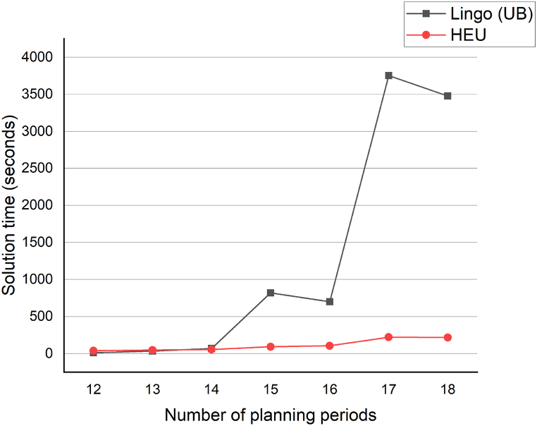
Table 4 displays the objective values and solution times for seven different problem instances. All instances feature eight farms but vary in planning periods, ranging from 12 to 18. Fig. 2 presents comparison graphs depicting the objective values of Lingo (LB), Lingo (UB), OPT, and HEU as obtained from Table 4. Similarly, Fig. 3 illustrates comparison graphs representing the solution times of Lingo (LB), Lingo (UB), OPT, and HEU, also derived from Table 4.
Table 4.
Objective values and solution time of 8-farm cases from period 12 to period 18.
| Objective value (unit cost) |
Solution time (sec.) |
||||||
|---|---|---|---|---|---|---|---|
| Problem Instances | Period | Lingo (LB) | Lingo (UB) | OPT | HEU | Lingo (UB) | HEU |
| 8F–12P | 12 | 714020 | 714020 | 714020 | 714020 | 13 | 40 |
| 8F–13P | 13 | 702898 | 702898 | 702898 | 702981 | 35 | 48 |
| 8F–14P | 14 | 709285 | 709285 | 709285 | 709662 | 68 | 57 |
| 8F–15P | 15 | 681264 | 681264 | 681264 | 681596 | 821 | 94 |
| 8F–16P | 16 | 698942 | 698942 | 698942 | 698942 | 701 | 107 |
| 8F–17P | 17 | 631255 | 646806 | a | 646806 | 3755 | 222 |
| 8F–18P | 18 | 685145 | 694729 | a | 694729 | 3480 | 219 |
No optimal solution found within 2 h.
Fig. 2.
Objective value comparison between Lingo (LB), Lingo (UB), OPT and HEU.
Fig. 3.
Solution time comparison between Lingo (UB) and HEU.
6.2.2. Results of 10-farm cases from period 12 to period 18
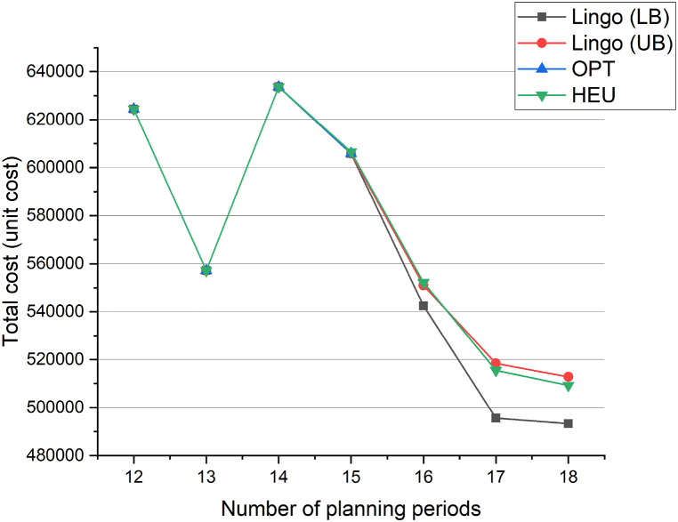
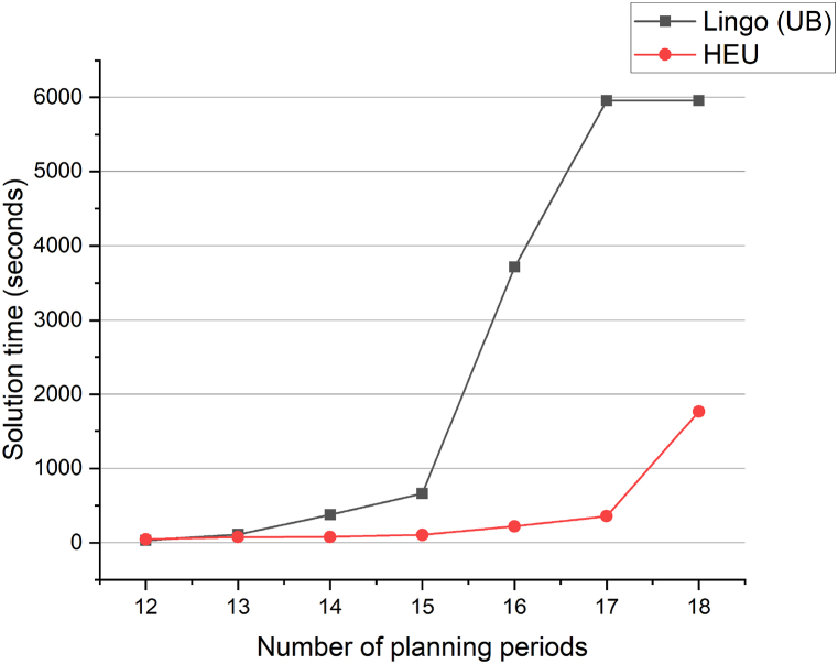
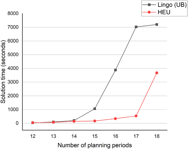
Table 5 displays the objective values and solution times for seven different problem instances. All instances feature ten farms but vary in planning periods, ranging from 12 to 18. Fig. 4 presents comparison graphs depicting the objective values of Lingo (LB), Lingo (UB), OPT, and HEU as obtained from Table 5. Similarly, Fig. 5 illustrates comparison graphs representing the solution times of Lingo (LB), Lingo (UB), OPT, and HEU, also derived from Table 5.
Table 5.
Objective values and solution time of 10-farm cases from period 12 to period 18.
| Objective value (unit cost) |
Solution time (sec.) |
||||||
|---|---|---|---|---|---|---|---|
| Problem Instances | Period | Lingo (LB) | Lingo (UB) | OPT | HEU | Lingo (UB) | HEU |
| 10F–12P | 12 | 624411 | 624411 | 624411 | 624411 | 31 | 47 |
| 10F–13P | 13 | 557160 | 557160 | 557160 | 557160 | 113 | 77 |
| 10F–14P | 14 | 633693 | 633693 | 633693 | 633693 | 378 | 79 |
| 10F–15P | 15 | 605843 | 605843 | 605843 | 606582 | 662 | 107 |
| 10F–16P | 16 | 542424 | 550939 | a | 552146 | 3715 | 221 |
| 10F–17P | 17 | 495584 | 518455 | a | 515558 | 5960 | 357 |
| 10F–18P | 18 | 493273 | 512845 | a | 509247 | 5959 | 1767 |
No optimal solution found within 2 h.
Fig. 4.
Objective value comparison between Lingo (LB), Lingo (UB), OPT and HEU.
Fig. 5.
Comparison between Lingo (UB) and HEU.
6.2.3. Results of 12-farm cases from period 12 to period 18
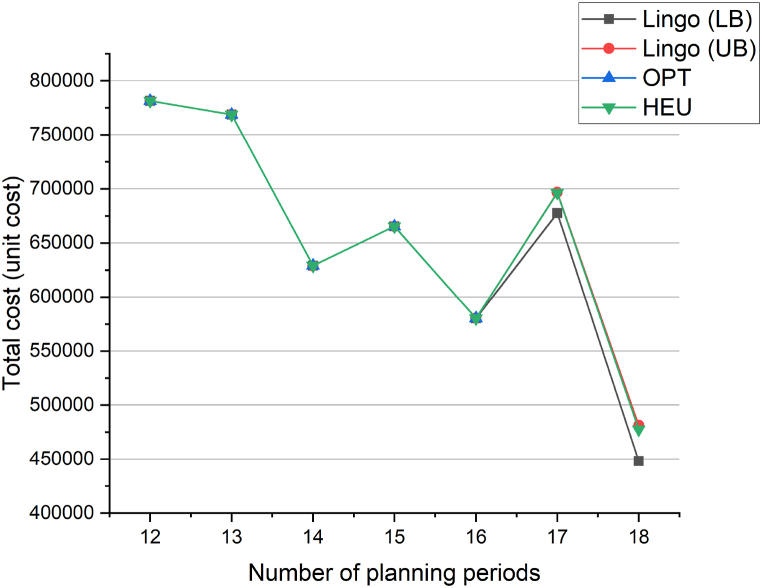
Table 6 displays the objective values and solution times for seven different problem instances. All instances consist of twelve farms but vary in planning periods, ranging from 12 to 18. Fig. 6 presents comparison graphs depicting the objective values of Lingo (LB), Lingo (UB), OPT, and HEU as obtained from Table 6. Similarly, Fig. 7 illustrates comparison graphs representing the solution times of Lingo (LB), Lingo (UB), OPT, and HEU, also derived from Table 6.
Table 6.
Objective values and solution time of 12-farm cases from period 12 to period 18.
| Objective value (unit cost) |
Solution time (sec.) |
||||||
|---|---|---|---|---|---|---|---|
| Problem Instances | Period | Lingo (LB) | Lingo (UB) | OPT | HEU | Lingo (UB) | HEU |
| 12F–12P | 12 | 781482 | 781482 | 781482 | 781482 | 34 | 47 |
| 12F–13P | 13 | 768791 | 768791 | 768791 | 768889 | 96 | 70 |
| 12F–14P | 14 | 628925 | 628925 | 628925 | 628925 | 197 | 143 |
| 12F–15P | 15 | 665235 | 665235 | 665235 | 665235 | 1063 | 167 |
| 12F–16P | 16 | 580220 | 580220 | 580220 | 580220 | 3878 | 336 |
| 12F–17P | 17 | 677556 | 696670 | a | 696328 | 7026 | 536 |
| 12F–18P | 18 | 448200 | 481232 | a | 477501 | 7200 | 3677 |
No optimal solution found within 2 h.
Fig. 6.
Comparison between Lingo (LB), Lingo (UB), OPT and HEU.
Fig. 7.
Comparison between Lingo (UB) and HEU.
According to the computational results of all three case studies (8-farm, 10-farm, and 12-farm), our proposed heuristic algorithm was able to find optimal solutions, particularly when the number of planning periods was below 15. However, in instances where the optimal solution could not be found within 2 h, the objective values obtained using our proposed algorithm were slightly better than the objective value of the best feasible solution obtained using Lingo. Furthermore, in the majority of cases, the solution time of our proposed heuristic algorithm was shorter than that of Lingo. These results demonstrate the efficiency and effectiveness of our heuristic approach in solving the given problem instances.
7. Sensitivity analysis
In this section, a sensitivity analysis was conducted to validate the proposed algorithm and gain managerial insights by varying some input parameters of the model. Two case studies with 10 and 12 farms, respectively, and 12 planning periods from Section 6 were selected. These case studies were used to generate four additional case studies by modifying the pig's average demand rate per period by 10% and 20% for each case.
For each case study, five simulated instances of data were generated, and our proposed heuristic algorithm was employed to solve these instances. The average values of various cost measures, including the total inventory cost at the farm, the total inventory cost at the feed mill, the setup cost at the feed mill, the total cost at the feed mill, and the total cost of the supply chain, were recorded for each case study. The results of the sensitivity analysis are presented in Table 7. The corresponding charts and analyses of the results are provided in the subsequent subsections, offering insights into the performance of the proposed algorithm under different parameter variations.
Table 7.
Sensitivity analysis results.
| Types | Farm | Cost from different demand variations (unit cost) | ||||
|---|---|---|---|---|---|---|
| of cost | variations | −20% | −10% | 0% | 10% | 20% |
| Inventory | 10-Farm | 416240 | 392696 | 357346 | 321591 | 270725 |
| Cost (Farm) | 12-Farm | 608575 | 567262 | 518310 | 436884 | 436884 |
| Inventory | 10-Farm | 215880 | 211651 | 208520 | 207542 | 207564 |
| Cost (Feed) | 12-Farm | 204645 | 201719 | 204024 | 203203 | 203203 |
| Setup Cost | 10-Farm | 56084 | 54626 | 58545 | 58864 | 60303 |
| (Feed) | 12-Farm | 56008 | 55560 | 59147 | 60174 | 60174 |
| Total Cost | 10-Farm | 271965 | 266278 | 267065 | 266406 | 267867 |
| (Feed) | 12-Farm | 260652 | 257279 | 263171 | 263377 | 263377 |
| Total Cost | 10-Farm | 688205 | 658974 | 624411 | 587997 | 538592 |
| 12-Farm | 869227 | 824542 | 781482 | 700261 | 700261 | |
7.1. Inventory cost at the farms
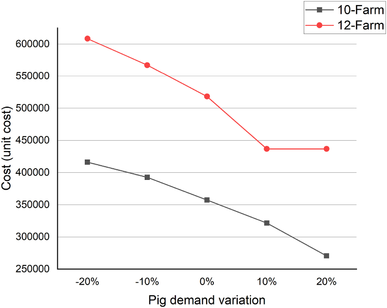
The graphs in Fig. 8 depict the results of the sensitivity analysis for both the 10-farm and 12-farm cases. They illustrate the relationship between the total inventory cost at the farm and the demand for pigs. The graphs demonstrate that as the demand for pigs increases, the total inventory cost at the farm decreases. This is because the proposed model does not consider the setup cost at the farm, and the quantity of pigs in inventory is solely determined by the farm size and the pigs' demand. Consequently, as the demand for pigs increases, farms can reduce their inventory levels, resulting in lower inventory costs.
Fig. 8.
The total inventory cost at the farm.
Additionally, it can be observed that the 12-farm graph lies above the 10-farm graph. This is because as the number of farms increases, the total inventory cost also increases. This is intuitive since more farms imply a greater number of pigs and hence higher inventory levels, leading to increased inventory costs. Overall, these findings highlight the inverse relationship between the total inventory cost at the farm and the demand for pigs, as well as the positive relationship between the number of farms and the total inventory cost.
7.2. Inventory cost at the feed mill
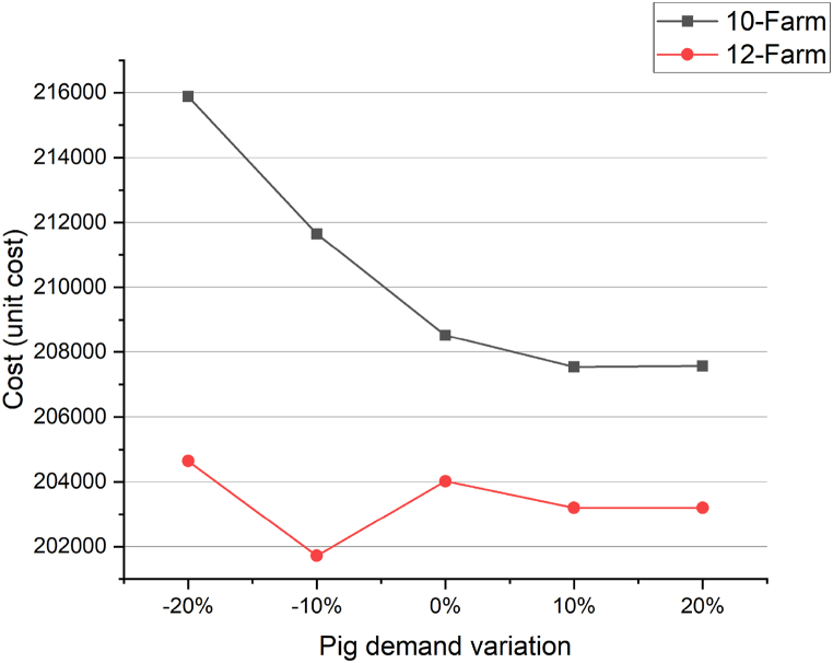
The chart in Fig. 9 presents the results of the sensitivity analysis for both the 10-farm and 12-farm cases, focusing on the relationship between the total inventory cost at the feed mill and the demand for pigs. According to the chart, it is evident that as the demand for pigs increases, the total inventory cost at the feed mill decreases. This can be attributed to the fact that when there is a higher demand for pigs, the feed inventory depletes more rapidly since more pigs are remaining on the farm. Consequently, the feed consumption rate increases, leading to a reduction in the total inventory cost at the feed mill.
Fig. 9.
The total inventory cost at the feed mill.
Furthermore, the chart also indicates that the 10-farm graph is positioned above the 12-farm graph. This disparity is due to the fact that the 10-farm cases involve a smaller number of pigs compared to the 12-farm cases. As a result, the feed consumption rate is higher in the 12-farm cases, resulting in a lower total inventory cost at the feed mill for the 10-farm cases.
7.3. Setup cost at the feed mill
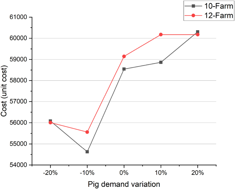
The chart in Fig. 10 illustrates the sensitivity analysis results for the total setup cost in both the 10-farm and 12-farm cases, considering the variation in the demand for pigs. According to the chart, there is an initial negative trend in the total setup cost as the demand for pigs increases. This suggests that when the demand for pigs rises the feed mill will need to switch between different feed formulations more frequently. As a result, the total setup cost decreases initially.
Fig. 10.
The total setup cost at the feed mill.
However, as the demand for pigs continues to increase, the trend in the total setup cost turns positive and begins to slow down towards the end. This indicates that there is a limit to the number of feed formulations that can be effectively switched between. Once this limit is reached, the increase in the demand for pigs leads to a higher total setup cost as the feed mill has to employ additional setups to accommodate the demand.
Furthermore, the chart also shows that the 12-farm graph is positioned above the 10-farm graph. This is because, in the 12-farm cases, there is a greater diversity of pigs of different ages. As a result, more setups are required to cater to the varying needs of these different age groups, resulting in a higher total setup cost compared to the 10-farm cases.
7.4. Total cost at the feed mill
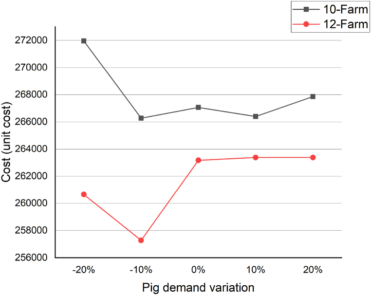
The graphs in Fig. 11 represent the sensitivity analysis results for the total costs in both the 10-farm and 12-farm cases, considering the variation in the demand for pigs. According to the graphs, there is a slight decline in the total costs at the beginning, followed by an upswing near the end. This can be attributed to the opposing trends of the inventory holding cost and the setup cost. The decline in total costs at the beginning can be attributed to the decrease in the inventory holding cost as the demand for pigs increases. As more pigs are consumed and fewer remain in inventory, the inventory holding cost decreases.
Fig. 11.
The total cost at the feed mill.
However, as the demand for pigs continues to increase, the setup cost begins to dominate the total costs. This leads to an upswing in the total costs as the feed mill needs to perform more frequent setups to meet the demand for different feed formulations. Additionally, the graphs indicate that the costs of the 10-farm cases are higher compared to the 12-farm cases. This is because the inventory holding cost significantly outweighs the setup cost, and the 10-farm cases have higher inventory holding costs due to fewer pigs in inventory compared to the 12-farm cases.
7.5. Total cost
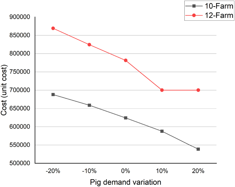
The chart in Fig. 12 presents the sensitivity analysis results for the total supply chain cost, considering the variation in the demand for pigs. According to the chart, the total supply chain cost exhibits a negative trend as the demand for pigs increases. This can be attributed to the combined effect of the individual cost trends at the farm and the feed mill. This is due to the fact that the inventory holding cost at the farm decreases when more pigs are sold, resulting in lower costs. On the other hand, the total cost at the feed mill has a primarily flat trend. This indicates that the changes in the feed mill's costs do not vary significantly with the demand for pigs. When these individual cost trends are combined, the overall effect is a negative trend in the total supply chain cost. The decreasing cost at the farm outweighs the relatively stable cost at the feed mill, resulting in a net reduction in the total supply chain cost as the demand for pigs increases.
Fig. 12.
The total cost of the supply chain.
8. Discussion and limitations
The study's methodology involved computational experiments applied to address challenges in a vertically integrated pig supply chain. We explored case studies consisting of various farm sizes, and various planning periods. Problem instances are defined by the number of farms (8, 10, and 12) and planning periods (12–18), leading to diverse scenarios for analysis. We generated comparative results between Lingo's Simplex solver [39] and our proposed heuristic. The proposed heuristic finds optimal solutions, especially for planning periods below 15, and in cases where Lingo fails to find an optimal solution within 2 h, the proposed heuristic demonstrates slightly better objective values. Additionally, the solution time for the proposed heuristic is observed to be generally shorter than that of Lingo's Simplex solver. Sensitivity analysis was conducted by adjusting the pig's average demand rate per period by 10% and 20% across various case studies. The outcomes unveiled crucial insights into the correlation among demand, inventory costs, and the number of farms. It was observed that an increase in pig demand resulted in reduced inventory costs at both farm and feed mill levels. Additionally, while the inventory cost of pigs tended to rise with a greater number of farms, the feed inventory cost demonstrated a tendency to decrease.
The study is subject to some limitations. Firstly, the problem's NP-hard classification contributes to increased computational complexity and solution time, especially concerning larger instances, thereby presenting scalability challenges for the proposed heuristic. This could limit the practicality of the proposed method. Moreover, the sensitivity analysis, although informative regarding cost parameters, was limited in scope as it concentrated solely on particular cost measures. This approach might have disregarded other crucial elements such as market dynamics or governmental policies. Lastly, the evaluation and comparison of the proposed heuristic with Lingo's solver were focused on specific performance metrics such as solution times and objective values. There might be additional metrics or criteria relevant to the supply chain (e.g., robustness, adaptability to dynamic scenarios) that were not thoroughly addressed.
9. Conclusion and future research
In conclusion, this study explored the complexities of a vertically integrated pork production supply chain consisting of a feed mill, multiple fattening farms responsible for delivering market-size pigs based on demand. The aim was to optimize production plans for these entities by proposing a mixed-integer linear programming model. Furthermore, a Lagrangian heuristic was developed to address this problem. Computational experiments were executed on diverse case studies involving various farm sizes and planning periods, facilitating a comparison between the proposed heuristic and Lingo's Simplex solver using identical datasets. Notably, it showed the capability to find optimal solutions quicker for smaller problem instances, and to produce more effective feasible solutions within limited time frames for larger scenarios. This study not only tackled the supply chain challenges effectively but also introduced an efficient heuristic approach, offering significant insights for supply chain managers and decision-makers.
In this study, we have proposed a mathematical model for integrating two production stages in a pig supply chain and employed a Lagrangian heuristic as the solution method. Our research has revealed limitations, including scalability issues in handling larger networks, which necessitate further investigation in future studies through exploration of alternative solution methods. Recent advancements in optimization algorithms, including hybrid heuristics, metaheuristics, and other adaptive algorithms, have gained prominence in addressing complex decision problems across domains that were previously deemed computationally infeasible. Notably, the Self-adaptive Fast Fireworks Algorithm (SF-FWA) offers a computationally efficient, general-purpose optimization approach suitable for large-scale tasks [41]. Another promising method is the Adaptive Polyploid Memetic Algorithm (APMA) [42], designed for truck scheduling in cross-docking environments, surpassing well-known metaheuristics in solution quality. Recent heuristics based on exact optimization methods, as seen in Ref. [43] addressing multi-objective vehicle routing problem, and [44] tackling level crossing safety issues with conflicting objectives, hold potential for addressing complex supply chain problems with limited resources.
Data availability statement
Data will be available on request.
CRediT authorship contribution statement
Thawee Nakrachata-Amon: Writing – review & editing, Writing – original draft, Visualization, Validation, Supervision, Software, Resources, Project administration, Methodology, Investigation, Funding acquisition, Formal analysis, Data curation, Conceptualization. Jumpol Vorasayan: Visualization, Validation, Supervision, Resources, Methodology, Conceptualization. Komkrit Pitiruek: Visualization, Validation, Supervision, Methodology, Investigation, Conceptualization. Sirawadee Arunyanart: Visualization, Validation, Supervision, Methodology, Investigation, Formal analysis, Conceptualization. Thanawath Niyamosoth: Visualization, Validation, Supervision, Methodology, Conceptualization. Supachai Pathumnakul: Writing – review & editing, Writing – original draft, Visualization, Validation, Supervision, Software, Resources, Project administration, Methodology, Investigation, Funding acquisition, Formal analysis, Data curation, Conceptualization.
Declaration of competing interest
The authors declare that they have no known competing financial interests or personal relationships that could have appeared to influence the work reported in this paper.
References
- 1.OECD/FAO . OECD Publishing; Paris: 2023. OECD-FAO Agricultural Outlook 2023-2032. Oct. 27, 2023. [Online]. Available: [DOI] [Google Scholar]
- 2.Usda Livestock, Poultry . Foreign Agricultural Service; 2023. World Production, Markets, and Trade Report.https://apps.fas.usda.gov/psdonline/circulars/livestock_poultry.pdf [Online]. Available: Nov. 1, 2023. [Google Scholar]
- 3.MacDonald J.M. vol. 1. Oxford University Press; 2018. (CAFOs: Farm Animals and Industrialized Livestock Production). [Google Scholar]
- 4.Davis C.G., et al. Hog Production U.S. U.S. Department of Agriculture, Economic Research Service; August 2022. Rising Output and Changing Trends in Productivity Growth, ERR-308. [Google Scholar]
- 5.Rodríguez S.V., Luis M.P., Faulin J. New opportunities in operations research to improve pork supply chain efficiency. Ann. Oper. Res. 2014;219:5–23. [Google Scholar]
- 6.Reimer J.J. Vertical integration in the pork industry. Am. J. Agric. Econ. 2006;88(1):234–248. [Google Scholar]
- 7.Ittiphalin M., Nakrachata-Amon T., Pathumnakul S. Feed formulation under raw material and production costs consideration. Appl. Mech. Mater. 2015;781:667–670. [Google Scholar]
- 8.Khamjan S., Piewthongngam K., Pathumnakul S. Pig procurement plan considering pig growth and size distribution. Comput. Ind. Eng. 2013;64(4):886–894. [Google Scholar]
- 9.Praseeratasang N., Pitakaso R., Sethanan K., Kaewman S., Golinska-Dawson P. Adaptive large neighborhood search for a production planning problem arising in pig farming. Journal of Open Innovation: Technology, Market, and Complexity. 2019;5(2):26. [Google Scholar]
- 10.USDA . USDA APHIS Veterinary Services; 2011. Swine Industry Manual. Foreign Animal Disease Preparedness and Response Plan.https://www.aasv.org/documents/swineindustrymanual.pdf [Online]. Available: [Google Scholar]
- 11.Millet S., et al. How two concurrent pandemics put a spoke in the wheel of intensive pig production. Animal Frontiers. 2021;11(1):14–18. doi: 10.1093/af/vfaa051. [DOI] [PMC free article] [PubMed] [Google Scholar]
- 12.Zhai T., Wang D., Zhang Q., Saeidi P., Mishra A.R. Assessment of the agriculture supply chain risks for investments of agricultural small and medium-sized enterprises (SMEs) using the decision support model. Economic Research-Ekonomska Istraživanja. 2023;36(2) [Google Scholar]
- 13.Solano-Blanco A.L., González J.E., Medaglia A.L. Production planning decisions in the broiler chicken supply chain with growth uncertainty. Operations Research Perspectives. 2023;10 [Google Scholar]
- 14.Nadal-Roig E., Plà-Aragonès E., L M., Pagès-Bernaus A., Albornoz V.M. A two-stage stochastic model for pig production planning in vertically integrated production systems. Comput. Electron. Agric. 2020;176 [Google Scholar]
- 15.Villalba D., Díez-Unquera B., Carrascal A., Bernués A., Ruiz R. Multi-objective simulation and optimisation of dairy sheep farms: exploring trade-offs between economic and environmental outcomes. Agric. Syst. 2019;173:107–118. [Google Scholar]
- 16.Han J.H., Kim Y.D. Design and operation of a two-level supply chain for production-time-dependent products using Lagrangian relaxation. Comput. Ind. Eng. 2016;96:118–125. [Google Scholar]
- 17.Peres F., Castelli M. Combinatorial optimization problems and metaheuristics: review, challenges, design, and development. Appl. Sci. 2021;11(14):6449. [Google Scholar]
- 18.Belvaux G., Wolsey L.A. Modelling practical lot-sizing problems as mixed-integer programs. Manag. Sci. 2001;47:993–1007. [Google Scholar]
- 19.Brahimi N., Absi N., Dauzère-Pérès S., Nordli A. Single-item dynamic lot-sizing problems: an updated survey. Eur. J. Oper. Res. 2017;263(3):838–863. [Google Scholar]
- 20.Bruno G., Genovese A., Piccolo C. The capacitated Lot Sizing model: a powerful tool for logistics decision making. Int. J. Prod. Econ. 2014;155:380–390. [Google Scholar]
- 21.Karimi B., F Ghomi S.M.T., Wilson J.M. The capacitated lot sizing problem: a review of models and algorithms. Omega. 2003;31(5):365–378. [Google Scholar]
- 22.Lai D., Li Y., Demir E., Dellaert N., Woensel T.V. Self-adaptive randomized constructive heuristics for the multi-item capacitated lot sizing problem. Comput. Oper. Res. 2022;147 [Google Scholar]
- 23.Bing-hai Z., Meng Y., Zhi-qiang L. An improved Lagrangian relaxation heuristic for the scheduling problem of operating theatres. Comput. Ind. Eng. 2016;101:490–503. [Google Scholar]
- 24.Özyurt Z., Aksen D. Solving the multi-depot location-routing problem with Lagrangian relaxation. Oper. Res./Comput. Sci. Inf. Syst. 2007;37:125–144. [Google Scholar]
- 25.Imai A., Nishimura E., Current J. A Lagrangian relaxation-based heuristic for the vehicle routing with full container load. Eur. J. Oper. Res. 2007;176(1):87–105. [Google Scholar]
- 26.Kim J.U., Kim Y.D. A Lagrangian relaxation approach to multi-period inventory/distribution planning. J. Oper. Res. Soc. 2017;51(3):364–370. [Google Scholar]
- 27.Rizk N., Martel A., Ramudhin A. A Lagrangean relaxation algorithm for multi-item lot-sizing problems with joint piecewise linear resource costs. Int. J. Prod. Econ. 2006;102(2):344–357. [Google Scholar]
- 28.Berretta R., França P.M., Armentano V.A. Metaheuristic approaches for the multilevel resource-constrained lot-sizing problem with setup and lead times. Asia Pac. J. Oper. Res. 2005;22:261–286. [Google Scholar]
- 29.Bassey U., Zelibe S. Two-echelon inventory location model with response time requirement and lateral transshipment. Heliyon. 2022;8(8) doi: 10.1016/j.heliyon.2022.e10353. [DOI] [PMC free article] [PubMed] [Google Scholar]
- 30.Nikzad P., Min H., Moghadam F.Y. Redesigning multi-echelon integrated distribution networks using the Lagrangian relaxation heuristics. Eur. J. Ind. Eng. 2021;15(3):352–380. [Google Scholar]
- 31.Fisher M.L. An applications oriented guide to Lagrangian relaxation. Interfaces. 1985;15(2):10–21. [Google Scholar]
- 32.Fisher M.L. The Lagrangian relaxation method for solving integer programming problems. Manag. Sci. 2004;50(12):1861–1874. [Google Scholar]
- 33.Jeet V., Kutanoglu E. Lagrangian relaxation guided problem space search heuristics for generalized assignment problems. Eur. J. Oper. Res. 2007;182:1039–1056. [Google Scholar]
- 34.Létocart L., Nagih A., Touati-Moungla N. Dantzig-Wolfe and Lagrangian decompositions in integer linear programming. Int. J. Math. Oper. Res. 2012;4(3):247–262. [Google Scholar]
- 35.Guignard M., Kim S. Lagrangean decomposition for integer programming: theory and applications. Oper. Res. 1987;21(4):307–323. [Google Scholar]
- 36.Reinoso H., Maculan N. Lagrangean decomposition in integer linear programming: a new scheme. INFOR Inf. Syst. Oper. Res. 1992;30(1):1–5. [Google Scholar]
- 37.Visweswaran V. Decomposition techniques for MILP: Lagrangian relaxation. Encyclopedia of Optimization. 2009:632–638. [Google Scholar]
- 38.Guignard M., Kim S. Lagrangean decomposition: a model yielding stronger lagrangean bounds. Math. Program. 1987;39(2):215–228. [Google Scholar]
- 39.LINGO User's Manual. LINGO System Inc.; 2012. (version 13) [Google Scholar]
- 40.Hasan R.B., Osman H., Azab A., Baki F. Improvement to an existing multi-level capacitated lot sizing problem considering setup carryover, backlogging, and emission control. Manufacturing Letters. 2023;35:28–39. [Google Scholar]
- 41.Chen M., Tan Y. A self-adaptive Fast Fireworks algorithm for effective large-scale optimization. Swarm Evol. Comput. 2023;80 [Google Scholar]
- 42.Dulebenets M.A. An Adaptive Polyploid Memetic Algorithm for scheduling trucks at a cross-docking terminal. Inf. Sci. 2021;565:390–421. [Google Scholar]
- 43.Pasha J., Nwodu A.L., Fathollahi-Fard A.M., Tian G., Li A., Wang H., Dulebenets M.A. Exact and metaheuristic algorithms for the vehicle routing problem with a factory-in-a-box in multi-objective settings. Adv. Eng. Inf. 2022;52 [Google Scholar]
- 44.Singh P., Pasha J., Moses R., Sobanjo J., Ozguven E.E., Dulebenets M.A. Development of exact and heuristic optimization methods for safety improvement projects at level crossings under conflicting objectives. Reliab. Eng. Syst. Saf. 2022;220 [Google Scholar]
Associated Data
This section collects any data citations, data availability statements, or supplementary materials included in this article.
Data Availability Statement
Data will be available on request.


