Increasing the Dissolution Rate of Polystyrene Waste in Solvent-Based Recycling

Abstract

Solvent-based recycling of plastic waste is a promising approach for cleaning polymer chains without breaking them. However, the time required to actually dissolve the polymer in a lab environment can take hours. Different factors play a role in polymer dissolution, including temperature, turbulence, and solvent properties. This work provides insights into bottlenecks and opportunities to increase the dissolution rate of polystyrene in solvents. The paper starts with a broad solvent screening in which the dissolution times are compared. Based on the experimental results, a multiple regression model is constructed, which shows that within several solvent properties, the viscosity of the solvent is the major contributor to the dissolution time, followed by the hydrogen, polar, and dispersion bonding (solubility) parameters. These results also indicate that cyclohexene, 2-pentanone, ethylbenzene, and methyl ethyl ketone are solvents that allow fast dissolution. Next, the dissolution kinetics of polystyrene in cyclohexene in a lab-scale reactor and a baffled reactor are investigated. The effects of temperature, particle size, impeller speed, and impeller type were studied. The results show that increased turbulence in a baffled reactor can decrease the dissolution time from 40 to 7 min compared to a lab-scale reactor, indicating the importance of a proper reactor design. The application of a first-order kinetic model confirms that dissolution in a baffled reactor is at least 5-fold faster than that in a lab-scale reactor. Finally, the dissolution kinetics of a real waste sample reveal that, in optimized conditions, full dissolution occurs after 5 min.

Short abstract

The dissolution of polystyrene is achieved in 7 min, enhancing the industrial implementation of dissolution recycling of plastic waste.

1. Introduction

Polymer dissolution plays an important role in several industrial applications, such as drug delivery, microlithography, membrane science, and dissolution recycling.¹ In solvent-based recycling (also known as dissolution recycling), the first step is the dissolution of the polymer in a suitable solvent, which is then followed by several cleaning steps for the removal of additives and contaminants. The process ends with a precipitation step to recover the polymer from the solution.² The choice of a proper solvent for the polymer plays an important role in the overall cost efficiency of solvent-based recycling.

In the case of solvent-based recycling, it is crucial for the industry to have a fast dissolution process, without waiting hours before the dissolution of the polymer, which would require excessive reactor volumes to create throughput. The dissolution of a polymer is a complex process and it involves several mass transfer processes.¹ For a non-cross-linked, amorphous, and glassy polymer such as polystyrene (PS), the dissolution process starts with the diffusion of the solvent into the polymer, followed by the swelling of the polymer, which forms a gel-like rubbery swollen layer.^3,4 This swollen gel layer has two interfaces: one between the glassy polymer and the gel layer and the other between the gel layer and the solvent. After an induction time, the polymer chains disentangle from the surface of the swollen polymer and the solvated polymer molecules are dispersed in the solution, as schematically depicted in Figure 1.^1,5

Figure 1.

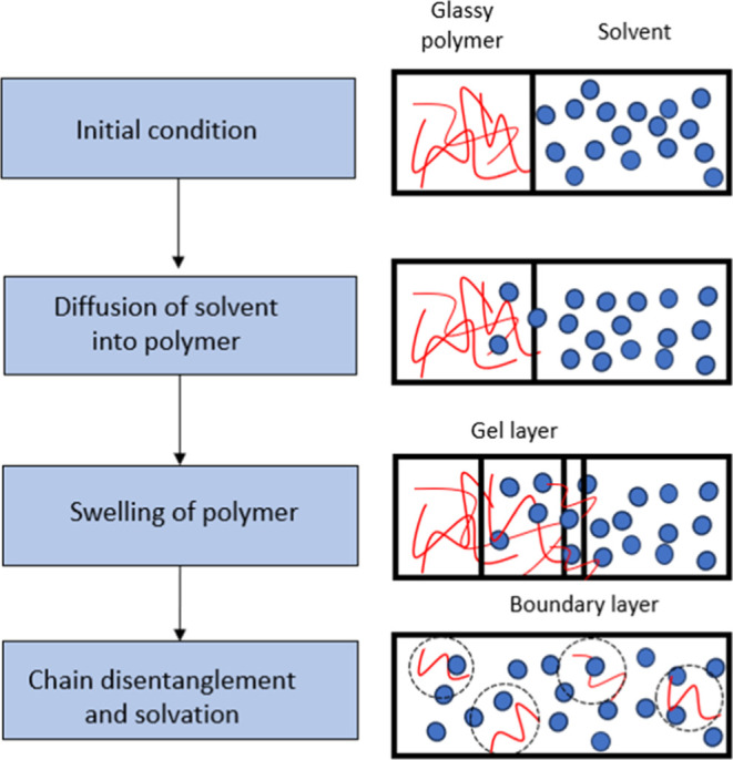
Schematic representation of the dissolution process for polymer molecules (non-cross-linked, amorphous, and glassy states). Reprinted with permission from ref (6). Copyright 2014 Royal Society of Chemistry.

The dissolution of polymers is influenced by several factors, namely the polymer properties, such as (average) molar mass, polydispersity, polymer structure, composition, conformation, particle size, solvent, and presence of additives, as well as external parameters, such as stirring and temperature.^1,7,8 In the literature, it has been observed that the controlling step varies depending on the polymer–solvent system.⁴ For example, the dissolution of polymers with high (average) molar mass is controlled by disentanglement of the chains rather than by diffusion. Narasimhan and Peppas⁹ studied the dissolution of polystyrene in methyl ethyl ketone and observed that the dissolution mechanism became disentanglement-controlled upon increasing the (average) molar mass of the polymer. This is related to the time required for a polymer chain to completely diffuse out of the reptation tube. However, in a more recent work by Valois et al.,¹⁰ it was observed that the relaxation mechanism of polymer chains is a consequence of chain contraction in the tubes, which is fast and thus not a limiting step. Instead, dissolution without stirring is limited by the lifetime of the transiently formed gel. The dissolution is complete when the gel turns into a diluted solution in which the polymers are dispersed by natural convection. This implies that complete dissolution occurs when the overlap concentration is reached, which defines the transition between the dilute and semidilute unentangled regions. Zhang et al.¹¹ studied the dissolution behavior of polystyrene in biodiesel and observed that the overall dissolution rate of PS appears to be controlled by the diffusion of polymer chains through a boundary layer adjacent to the polymer/solvent interface, which occurs after the disentanglement step.

However, when stirring is involved, it has been observed that the gel layer is decreased and in some cases not completely formed because the agitation strips off the gel layer,^1,10 which means that the swelling step, as shown in Figure 1, is negligible. The concentration at which the gel erodes is dependent on the shear rate and increases with increasing shear rate.¹⁰ An increase in temperature results in a faster disentanglement of the polymer chains and therefore higher dissolution rates.¹¹ In the literature, it has been observed that the overlap concentration varies only slightly with temperature.¹² Similarly, the entanglement concentration, which is defined as the transition between the semidilute entangled to a semidilute unentangled region, was also found not to change significantly with temperature.^12,13 Most of these studies focus on generating an in-depth understanding of the dissolution process, mainly in a lab environment, but based on a limited set of solvents. The influence of a proper reactor design and impeller type on polymer dissolution kinetics has not been compared to that of lab-scale reactors. Furthermore, the development of a regression model to understand the influence of solvent properties on the dissolution kinetics of the polymer is also very relevant to facilitate solvent choice without the need to extensively record experimental data. Moreover, these studies usually focused on pure polymers, whereas the dissolution kinetics of real waste samples, relevant to solvent-based recycling, have not been investigated.

The objective of this work is to provide evidence for factors that increase the dissolution rate of plastic waste, particularly polystyrene. For this purpose, screening of promising solvents for polystyrene was performed as a first step. Based on this, a regression model was developed that provided evidence of the influence of solvent properties on dissolution kinetics. Next, the effects of particle size, temperature, and reactor conditions, such as impeller type and impeller speed on the dissolution kinetics of polystyrene, were studied. Finally, dissolution kinetics were quantified using a real waste sample.

2. Materials and Methods

2.1. Materials

Polystyrene pellets (General Purpose Polystyrene “GPPS”: Styrolution PS 168 N) were kindly provided by INEOS Styrolution. Several solvents were chosen to study the dissolution of polystyrene. The solvents tested were acetone (ChemLab, >99.5%), α-methylstyrene (ThermoFisher Scientific, 99%), anisole (SigmaAldrich, 99%), benzaldehyde (SigmaAldrich, >99%), benzyl alcohol (SigmaAldrich, 99.8%), benzyl benzoate (SigmaAldrich, >99%), butyl benzoate (SigmaAldrich, 99%), n-butyl acetate (ThermoFisher Scientific, 99%), cyclohexane (ChemLab, >99.5%), cyclohexanol (ChemLab, >99%), cyclohexanone (ChemLab, >99%), cyclohexene (ChemLab, >99%), dibenzyl ether (ThermoFisher Scientific, >98%), diethyl carbonate (SigmaAldrich, 99%), diethylene glycol monobutyl ether (DGME) (SigmaAldrich, >99%), diphenyl ether (ThermoFisher Scientific, 99%), ethyl acetate (ChemLab, >99.5%), ethylbenzene (SigmaAldrich, >99%), ethyl formate (ThermoFisher Scientific, 97%), geranyl acetate (SigmaAldrich, 90%), isoamyl acetate (SigmaAldrich, >97%), isobutyl acetate (ThermoFisher Scientific, 98%), isobutyl isobutyrate (ThermoFisher Scientific, 98%), d-limonene (ThermoFisher Scientific, 96%), methyl benzoate (ThermoFisher Scientific, 99%), methyl ethyl ketone (MEK) (ChemLab, >99.5%), methyl-p-toluate (ThermoFisher Scientific, 99%), 2-pentanone (ThermoFisher Scientific, 99%), phenyl acetate (ThermoFisher Scientific, 97%), o-xylene (ThermoFisher Scientific, 99%), xylene isomer mixture (ChemLab, >99%), tetrahydrofuran (THF) (SigmaAldrich, >99%), and 1,2,3,4-tetrahydronaphthalene (ThermoFisher Scientific, 97%).

The waste sample used in this study was PS from foamed fish boxes collected from a sorting facility as a large nonwashed compressed block. The waste PS was washed in a washing machine without detergent in a 30 min cycle at a low temperature (35 °C). The waste PS was then dried in a drying machine with a short cycle (12 min) at 55 °C and left for 2 days in an oven at 60 °C until the mass was constant. To reduce the particle size, the waste PS was shredded using an 8 mm sieve (Shini Plastic Technologies, SG-1635N-CE), and to obtain a narrower particle size distribution, the shredded waste PS was sieved using a sieve shaker with 1.18 and 2.0 mm sieves (Endecotts LTD).

2.2. Screening of Best Solvents for Polystyrene

2.2.1. Hansen Solubility Parameter

First, solvent screening for polystyrene dissolution was performed using Hansen solubility parameters (HSP), which uses spheres for polymers to show their solubility range in solvents, represented by dots, in a three-dimensional graph. The suitability of a solvent to dissolve a polymer can be assessed by calculating the distance between the solubility parameters of a solvent and polymer, Ra, which is given by eq 1.¹⁴

1

where δ_D is the dispersion cohesion (solubility) parameter [MPa^1/2], δ_P is the polar cohesion (solubility) parameter [MPa^1/2], δ_H is the hydrogen bonding cohesion (solubility) parameter [MPa^1/2], and subscripts P and S refer to the polymer and solvent, respectively.

Next, the relative energy difference (RED) value was calculated, which is given by the ratio of Ra to the radius of the polymer interaction sphere in the Hansen space, Ro, and indicates the affinity between the polymer and the solvent. A RED value smaller than 1 indicates that the polymer and solvent have a high affinity, implying that the solvent will likely dissolve the polymer.¹⁴ The HSP of the solvents were taken from the literature¹⁴ as well as the HSP and Ro of polystyrene, the latter being δ_D = 21.3 MPa^1/2, δ_P = 5.8 MPa^1/2, δ_H = 4.3 MPa^1/2, and Ro = 12.7 MPa^1/2.

The RED values were calculated for 455 solvents for which the HSP parameters are available in the literature.¹⁴ To reduce the total number of solvents, several criteria were used: (i) the RED values (solvents with the lowest RED value were included but also solvents with RED values close to 1, so that the spectrum is broadened for the regression analysis in Section 2.2.3), (ii) acids, bases, halogenated solvents, and restricted solvents under the REACH regulation (EC 1907/2006)¹⁵ (e.g., benzene) were excluded, (iii) the cost/availability in the market was considered, and (iv) the boiling point of the solvent was also taken into account, e.g., solvents with BP < 50 °C were excluded. Based on these criteria, 33 solvents were selected for experimental validation.

2.2.2. Experimental Solvent Validation

First, the received polystyrene pellets were sieved using a sieve shaker (Endecotts LTD) for 10 min to obtain pellets with narrower particle size distribution between 2.36 and 5.6 mm. Depending on the solvent density, approximately 1 g of polymer was placed inside a vial. Afterward, 10 mL of solvent was added to the vial, and dissolution was started for 30 min, with magnetic stirring, in a thermostatic bath at 50 °C for each of the 33 selected solvents. The amount of dissolved polystyrene in the clear supernatant was then quantified by using thermogravimetric analysis (TGA). TGA measurements were carried out in a Netsch TG 209 F3 Tarsus thermogravimeter under a constant flow of dry nitrogen at a rate of 20 mL·min^–1. The temperature profile was as follows: a dynamic step from 35 to 250 °C at 15 °C·min^–1, followed by an isothermal step at 250 °C for 15 min, a dynamic step up to 600 °C at 100 °C·min^–1, followed by a dynamic step at 20 °C·min^–1 until 700 °C. The mean absolute error associated with TGA measurements is 0.09 wt % and the standard deviation is 0.08 wt %.¹³ In most cases, the polymer pellets were not completely dissolved, so part of the clear supernatant was pipetted out for polymer quantification analysis. A swollen polymer was obtained for acetone and ethyl formate. To ensure reproducibility, three experiments were performed in triplicate, and the relative standard deviation varied between 2.0 and 5.8% (Table S1, Supporting Information).

2.2.3. Regression Analysis for Polymer Dissolution

A multiple linear regression model with interaction terms was developed to assess the influence of solvent properties on the dissolution of polystyrene. The dependent variable is the concentration of dissolved polystyrene after 30 min of dissolution at 50 °C. The following solvent properties were included as independent variables: the dispersion cohesion (solubility) parameter, the polar cohesion (solubility) parameter, the hydrogen bonding cohesion (solubility) parameter, melting point, boiling point, molecular weight, flash point, viscosity at 50 °C, density at 50 °C, molar heat capacity at 50 °C, partition coefficient of the solvent between octanol and water, van der Waals volume, and heat of evaporation.

The solvent properties were either taken from the literature, measured, or calculated with molecular modeling software (Gaussian 16, COSMO-RS or ChemDraw). The specific heat capacity, van der Waals volume, surface area, dipole moment, polarizability, and solute radius were extracted from density functional theory (DFT), and the calculations were performed with Gaussian 16.¹⁶ The calculations were made using the B3LYP hybrid functional along with the 6-311++G (d,p) basis set,^17,18 which has a proven record for organic molecules.¹⁹ Furthermore, COSMO-RS files for the chemical compounds were generated by Gaussian 16 and processed with Biovia Cosmotherm 20.0.0 (Dassault Systèmes). The viscosity and density of the solvents were measured using an Anton Paar SVM 3001 viscometer at 50 °C. Three measurements were performed to ensure reproducibility. The retrieved solvent properties are summarized in Table 1.

Table 1. Solvent Properties^a.

solvent	CAS number	RED [–]	δD[MPa1/2]	δP[MPa1/2]	δH[MPa1/2]	MP[°C]	BP[°C]	Mw[g·mol–1]	FP[°C]	μ[MPa·s]	ρ[kg·m–3]	Cp[J·mol–1 K–1]c	log Pd	VdWvolume[cm3·mol–1]c	ΔHvap[kJ·mol–1]e
cyclohexene	110-83-8	0.75	17.2	1	5	–103.5	82.98	82.143	–6	0.397	783.51	89.8	2.99	74	33.57
2-pentanone	107-87-9	0.85	16	7.6	4.7	–78	102	86.13	7	0.313	777.380	110.5	0.857	111	38.4
ethylbenzene	100-41-4	0.72	17.8	0.6	1.4	–95	136	106.167	18	0.422	842.530	116.8	3.6	94	41
MEK	78-93-3	0.87	16	9	5.1	–87	80	72.11	–9	0.232	726.970	90.5	0.29	82	34
THF	109-99-9	0.62	17.8	5.7	8	–108	65	72.11	–14.5	0.274	801.550	71.2	0.45	54	32.16
ethyl acetate	141-78-6	0.90	15.8	5.3	7.2	–84	77	88.11	–4	0.249	863.060	102.1	0.73	69	35
xylene mixture	1330-20-7	0.70	17.6	1	3.1	–13	138	106.16	29	0.415	806.570	122.4	3.15	105	41.5
α-methylstyrene	98-83-9	0.54	18.5	2.4	2.4	–24	165	118.18	54	0.580	885.670	131.9	3.48	121	48.9
diethyl carbonate	105-58-8	0.98	15.1	6.3	3.5	–74	126	118.13	25	0.498	941.300	134.4	1.21	104	44.3
anisole	100-66-3	0.60	17.8	4.1	6.7	–37.3	155	108.14	52	0.670	967.380	110.6	2.62	93	44
o-xylene	95-47-6	0.67	17.8	1	3.1	–24	144	106.16	32	0.497	856.510	121.5	3.15	101	42
benzaldehyde	100-52-7	0.33	19.4	7.4	5.3	–26	178	106.12	63	1.141	1022.340	100.1	1.4	81	48
n-butyl acetate	123-86-4	0.90	15.8	3.7	6.3	–78	95	116.16	22	0.445	852.840	142.4	2.3	100	43
isobutyl acetate	110-19-0	1.00	15.1	3.7	6.3	–99	116	116.16	18	0.424	810.640	144.7	2.3	107	35.9
d-limonene	5989-27-5	0.72	17.2	1.8	4.3	–76	175	136.24	48	0.721	842.140	172.7	4.38	142	49.5
methyl benzoate	93-58-3	0.42	18.9	8.2	4.7	–15	199	136.15	83	1.182	1061.560	135.9	2.1	113	52
tetrahydronaphthalene	119-64-2	0.42	19.6	2	2.9	–35.8	207	132.2	77	1.265	943.420	136.7	3.78	100	55
methyl-p-toluate	99-75-2	0.37	19	6.5	3.8	32	222.4	150.177	95.5	1.543b	1057.238	161.1	2.34	118	53.5
isoamyl acetate	123-92-2	0.99	15.3	3.1	7	–78.5	142	130.19	25	0.530	845.280	164.8	2.7	105	46.4
phenyl acetate	122-79-2	0.29	19.8	5.2	6.4	–30	196	136.1	80	1.414	1050.380	138.4	1.49	101	53
isobutyl isobutyrate	97-85-8	1.01	15.1	2.9	5.9	–80.7	148.6	144.21	37	0.542	783.740	187.1	2.4	138	48.5
cyclohexanone	108-94-1	0.59	17.8	8.4	5.1	–32	155	98.15	44	1.262	921.760	103.5	0.86	67	44
cyclohexane	110-82-7	0.90	16.8	0	0.2	7	81	84.16	–18	0.564	733.340	95.0	3.44	94	33.1
geranyl acetate	105-87-3	0.92	15.8	2.27	5.69	<25	240	196.29	>93	1.560	899.260	257.9	4.04	151	58.1
butyl benzoate	136-60-7	0.48	18.3	5.6	5.5	–22.4	250	178.23	107	1.660	982.010	196.8	3.1	162	58.1
diphenyl ether	101-84-8	0.36	19.5	3.4	5.8	26.9	258	170.2	115	2.112	1050.520	167.6	4.21	149	64.2
dibenzyl ether	103-50-4	0.34	19.6	3.4	5.2	3.5	158	198.27	100	2.763	1022.140	206.7	3.31	148	45.6
benzyl alcohol	100-51-6	0.87	18.4	6.3	13.7	–15	205	108.14	93	2.735	1023.940	111.7	1.05	84	63
benzyl benzoate	120-51-4	0.22	20	5.1	5.2	18	323	212.25	148	4.065	1096.130	211.6	3.97	182	77.7
acetone	67-64-1	1.01	15.5	10.4	7	–95	56	58.08	–18	0.345b	803.491b	70.4	–0.23	45	31.27
ethyl formate	109-94-4	0.99	15.5	8.4	8.4	–80	54	74.08	–20	0.570b	970.513b	79.0	1.5	76	32.1
DGME	112-34-5	0.98	16	7	10.6	–68	231	162.229	78	2.885	936.540	205.8	1	149	55.7
cyclohexanol	108-93-0	0.96	17.4	4.1	13.5	25	161	100.158	68	10.939	927.690	115.1	1.25	86	62

^aLegend: δ_D -dispersion cohesion (solubility) parameter, δ_P - polar cohesion (solubility) parameter, δ_H - hydrogen bonding cohesion (solubility) parameter , MP - melting point, BP - boiling point, M_w - molecular weight, FP - flash point, μ - viscosity at 50 °C, ρ - density at 50 °C, C_p - molar heat capacity at 50 °C, log P - partition coefficient, VdW volume - van der Waals volume, ΔH_vap - heat of evaporation, MEK – methyl ethyl ketone, DGME – diethylene glycol monobutyl ether.

^bDue to the high volatility of these solvents, it was not possible to accurately measure their viscosity and density at 50 °C. These data were obtained from COSMO-RS.

^cGaussian 16 software.

^dRetrieved from the safety data sheet, and when not available, it was obtained from ChemDraw, which is the case for methyl-p-toluate, isobutyl isobutyrate, and butyl benzoate.

^eData from the NIST Chemistry Webbook. For the xylene isomer mixture, when not available, the data were calculated assuming the following composition: 0.4% m-xylene, 0.2% o-xylene, and 0.2% p-xylene.

A correlation matrix was established to check the relationship between the independent variables (solvent properties) and to eliminate highly correlated variables (Figure S1, Supporting Information).²⁰ The variables with the highest correlation were removed, and a multiple regression model was performed by removing the interaction terms with the highest p-value stepwise until only significant parameters (p < 0.05) remained. The script for the multiple linear regression model was prepared in R.(21)

2.3. Dissolution Kinetics

2.3.1. Lab-Scale Reactor: Influence of Particle Size and Temperature

The lab-scale kinetic experiments were carried out in a 250 mL round-bottom flask equipped with a reflux condenser, thermometer, overhead mechanical stirrer (Phoenix Instrument, RSO 20D) coupled with a two-pitched blade paddle-type impeller, and sampling inlet (Figure 2). A round-bottom flask containing the solvent (100 g) was placed in a thermostatic bath and preheated to the target temperature prior to the addition of the polymer.

Figure 2.

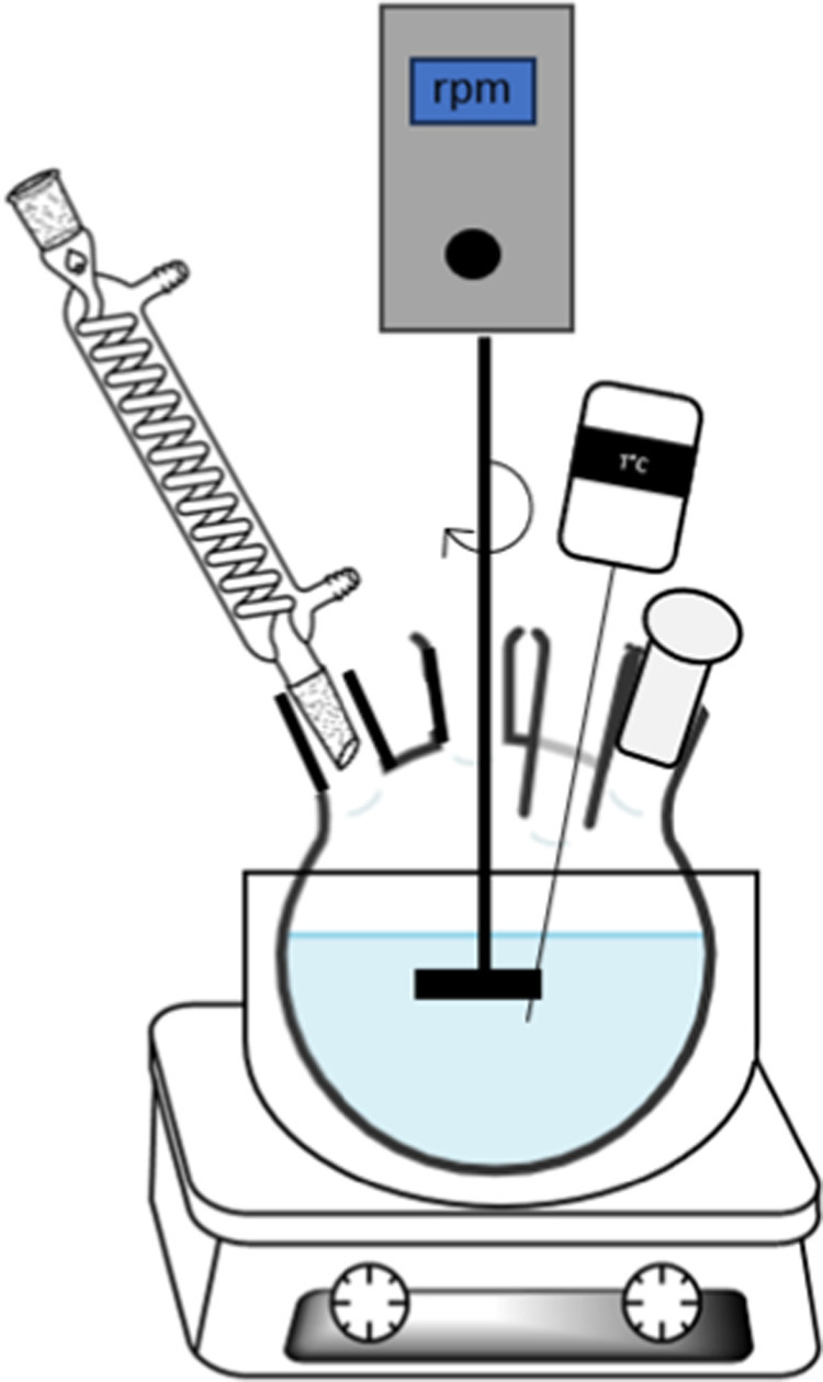
Schematic of the lab-scale reactor.

Approximately, 1 mL of liquid sample was collected over time until the concentration of the dissolved polymer reached a plateau. The dissolution kinetic experiments were performed with cyclohexene. The polymer concentration was measured over time by using a refractometer (Anton Paar, Abbemat) for which a calibration curve was prepared (Figure S2a, Supporting Information). A separate calibration curve was prepared for each waste sample (Figure S2b, Supporting Information).

Dissolution kinetic experiments were performed for solutions at 10 wt % at a fixed speed of 250 rpm under different experimental conditions, as defined by a full-factorial design. The design of experiments was constructed based on two factors, namely temperature (25, 50, and 75 °C) and particle size (1.0 < d_p < 1.18 mm, 1.18 < d_p < 2.0 mm, 2.0 < d_p < 2.36 mm). To obtain the different particle sizes, the received polystyrene pellets were pulverized (Fritsch, pulverizette 19) using a 750 μm sieve followed by sieving using a sieve shaker (Endecotts LTD) with 2.36, 2.0, 1.18, and 1.0 mm sieves for 10 min. Five replicates were performed in the experiment at 25 °C and a particle size fraction of 1.18 < d_p < 2.0 mm to ensure reproducibility of the results. The average relative standard deviation is 4.8% (Figure S3, Supporting Information).

For the purpose of determining the boundary of the concentration, the entanglement concentration of polystyrene in cyclohexene was considered at three different temperatures of 25, 50, and 75 °C (Figure S4, Supporting Information).¹³ The entanglement concentration was determined by measuring the viscosity as a function of the polymer concentration. Above the entanglement concentration, the presence of polymer entanglements is dominant, which consequently leads to a drastic increase in viscosity.¹³ The viscosities of different polystyrene solutions (1–25 wt %) were measured using an Anton Paar SVM 3001 viscometer at three temperatures: 25, 50, and 75 °C. Three measurements were performed to ensure reproducibility.

2.3.2. Baffled Reactor: Influence of Stirring and Impeller Type

Next, dissolution kinetic experiments were carried out in a double-walled thermostatic reaction vessel, which had a cylindrical shape with a dished bottom and a bottom valve. The reaction vessel was purchased from Glasaterlier Saillart and had a volume of 500 mL, a diameter of 100 mm, and a height of 170 mm. The reaction vessel contained 4 baffles pressed at a height of up to 90 mm and 12 mm deep, equipped with (i) a reflux condenser, (ii) an overhead mechanical stirrer (Velp Scientifica model OHS 200 Advance), coupled with an impeller, and (iii) a sampling inlet. Finally, the reaction vessel was connected to a temperature probe at the bottom of the reaction vessel and circulating heater (VWR Refrigerated Circulating Baths).

The liquid height was set equal to the reaction vessel diameter (Figure 3), following the geometric proportions for a standard agitation system.²² The impeller was mounted at a height equal to the diameter of the impeller, which was 38 mm for both impellers (Rushton turbine and propeller stirrer). The impellers were made of PTFE and produced by Bohlender.

Figure 3.

Side view of the reaction vessel (left), impellers (middle),²³ and geometric proportions.²²

Approximately, 1 mL of liquid sample was collected over time until the concentration of the dissolved polymer reached a plateau. Dissolution kinetics were performed with cyclohexene. The polymer concentration was measured over time using a refractometer and the calibration curves mentioned in Section 2.3.1.

Dissolution kinetic experiments were performed for solutions at 10 wt %, at a fixed temperature of 50 °C and a particle size fraction of 1.18 < d_p < 2.0 mm, under different experimental conditions, as defined by a full-factorial design. The design of experiments was constructed based on two factors: impeller speed (750, 875, 1000 rpm) and impeller type (Rushton turbine and propeller-stirrer shafts with 3 blades). These two impellers were chosen because they are suitable for viscosities in the range of 1 to 5 × 10⁴ mPa·s,²⁴ which covers the range expected for the studied polymer solutions. A higher impeller speed compared to the lab-scale reactor was used because at 250 rpm, the polymer particles settled on the bottom of the reactor, forming a gel layer that was difficult to dissolve. Five replicates were performed to ensure reproducibility of the results, and the average relative standard deviation was 1.8% for the experiment at 875 rpm with the propeller (Figure S5, Supporting Information).

2.3.3. Dissolution Kinetic Model

Kinetic models for the dissolution process are valuable tools to provide useful information for the design and optimization processes.²⁵ In this work, a first-order kinetics model is used,²⁶ since the aim of the paper is to understand which parameters are important for fast polymer dissolution, rather than understanding the subsequent steps of the dissolution process. The first-order kinetics equation is given by eq 2.²⁶

2

where Q_t is the amount of polymer dissolved in time t [wt %·min^–1], Q₀ is the initial concentration of polymer in the solution [wt %], and K₁ is the first-order dissolution constant [min^–1].

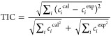
The model parameters were regressed by minimizing the sum of squares (SSE), as shown in eq 3. The performance of the model was evaluated by analyzing Theil’s inequality coefficient (TIC), eq 4. Modeling was performed using an in-house script in R using the flexible modeling environment (FME) package.²⁷

3

4

where c_i^exp is the experimental concentration of undissolved polystyrene and c_i^cal is the calculated value.

3. Results and Discussion

3.1. Solvent Screening

The results of solvent screening for polystyrene at 50 °C are summarized in Figure 4. The first dissolution screening results show that the solvents that dissolve the highest amount of polystyrene in 30 min are cyclohexene, 2-pentanone, ethylbenzene, and methyl ethyl ketone (MEK). THF and ethyl acetate also dissolve a high amount of polystyrene within this time frame. Some of the solvents did not dissolve polystyrene, leading to either a cloudy solution, swollen polymer, or undissolved pellets at 50 °C. This was the case for acetone, ethyl formate, diethylene glycol monobutyl ether (DGME), and cyclohexanol.

Figure 4.

Polystyrene concentrations in various solvents at 50 °C.

A regression model was developed based on these experiments, and the results are presented in Figure 5. Six independent variables were included in building the multiple regression model to predict the concentration of polystyrene based on the correlation matrix results (Figure S1). The solvent properties were normalized so that they were all within a comparable range, and a relative comparison of the variables was made. Additionally, the solvents were grouped into four representative categories: C1 – cyclic hydrocarbons, aromatic hydrocarbons, and aliphatic hydrocarbons; C2 – ethers and esters; C3 – aldehydes and ketones; and C4 – alcohols. The variables in the model are solvent partition coefficient, solvent-specific heat capacity, solvent viscosity, dispersion, polarity, and hydrogen cohesion (solubility). Figure 5 shows that the multiple regression model accurately predicted the concentration of polystyrene in different solvents, with an adjusted R² of 0.9443 and a p-value of 1.2 ·10^–10. The final equation of the model includes all of these variables (eq 5), with a residual standard error of 0.8 wt %.

5

where c is the concentration of the polymer [wt %], C2, C3, and C4 are the solvent categories [-], log P is the partition coefficient of the pure solvent [-], c_p is the specific heat capacity of the pure solvent [J·mol^–1·K^–1], η₀ is the viscosity of the pure solvent [Pa·s], δ_D is the dispersion cohesion (solubility) parameter of the pure solvent [MPa^1/2], δ_P is the polar cohesion (solubility) parameter of the pure solvent [MPa^1/2], δ_H is the hydrogen bonding cohesion (solubility) parameter of the pure solvent [MPa^1/2], and ε is the residual standard error [wt %].

Figure 5.

The results of the multiple regression model used to predict the concentration of polystyrene dissolved in different solvents at 50 °C.

The viscosity of the solvent has the largest regression coefficient and contributes negatively to the prediction of the concentration. This means that a solvent with a higher viscosity leads to a lower amount of dissolved polystyrene in the studied time frame, which relates to a lower diffusion coefficient, as it is inversely proportional to the viscosity of the liquid.¹ Next to viscosity, the dispersion cohesion (solubility) parameter has a positive contribution, while the polar and hydrogen bonding cohesion (solubility) parameters have a negative contribution. A solvent with a higher polar and hydrogen bonding cohesion (solubility) parameter has a higher polarity, which is typically the case for alcohols,¹⁴ and thus has a lower affinity for polystyrene, which decreases the diffusion coefficient.²⁸ Next, the heat capacity of the solvent has a negative contribution. The solvent-specific heat capacity can be related to the molecular weight and complexity of the molecule,²⁹ and thus this may indicate that a higher c_p (and thus a higher M_w) results in a lower dissolution rate.^1,30 Thermodynamically, c_p can be linked to the polymer–solvent interaction term, χ.^31,32 A higher c_p results in a higher χ and thus in a weaker polymer–solvent interaction, and consequently, in a lower dissolution rate.^3,28 Moreover, the c_p of the solvent is also an important parameter to be taken into account in solvent screening experiments since the solvent was not preheated during this screening (Section 2.2.2). The partition coefficient has a small and positive contribution, and it represents the ratio of the concentration of a solvent between two phases, octanol and water. A positive and high log P indicates a hydrophobic character and molecules with low or negative values are frequently considered polar.³³ Thus, this may indicate that solvents with lower or negative log P values will be more polar and thus have less affinity for polystyrene, which may be related to the dissolution rate.^3,28 Finally, the intercept term accounts for the reference category (C1) and serves as a baseline for comparison with the other category values. Thus, the regression coefficients of categories C2, C3, and C4 capture the differences of the expected values of these categories relative to the baseline (C1). For instance, in the case of C4, which represents alcohols, the intercept value is higher than that of C1 to account for the inherent differences in their characteristics (e.g., higher polarity and higher viscosity) that have a large negative effect on the dissolution of PS.

3.2. Dissolution Kinetics

3.2.1. Lab-Scale Reactor: Influence of Particle Size and Temperature

The entanglement concentration for the polystyrene solutions in cyclohexene is 13.8 wt % at 25 and 50 °C (Figure S4, Supporting Information). At 75 °C, it was not possible to accurately determine the entanglement concentration due to solvent evaporation. As previous results have shown that the entanglement concentration varies only slightly with temperature,¹³ it is assumed that 10 wt % is below the entanglement concentration at 75 °C. The results show that the complete dissolution of polystyrene in cyclohexene was observed after approximately 100 min at 25 °C, 40 min at 50 °C, and 30 min at 75 °C for the smallest particle size fraction of 1.0 < d_p < 1.18 mm (Figure 6). As expected, the dissolution time is higher for lower temperatures and larger particle sizes, although the time difference for complete dissolution does not differ much for different particle sizes. In the literature, this has been related to the existence of a polymer critical particle size, below which the dissolution is independent of the particle size.³⁴ This is especially relevant for industrial implementation since there is no need to spend more energy in reducing the particle size further.³⁴

Figure 6.

Dissolution results of polystyrene in cyclohexene at (a) 25 °C, (b) 50 °C, and (c) 75 °C for different particle size fractions.

3.2.2. Baffled Reactor: Influence of Stirring and Impeller Type

The dissolution experiments were performed in a baffled reactor at 50 °C for a particle size fraction of 1.18 < d_p < 2.0 mm and with two different impeller types, namely a Rushton turbine and a propeller-stirrer shaft with 3 blades. The results show that dissolution with the Rushton turbine is independent of stirring velocity (Figure 7). After approximately 7 min, full dissolution is achieved with a Rushton turbine. With the propeller, dissolution at 750 rpm was longer than that at higher impeller speeds. With the propeller at 875 and 1000 rpm, full dissolution is also achieved after approximately 7 min. Compared to dissolution in the lab-scale reactor, these results show that a proper reactor design is essential for optimized dissolution.

Figure 7.

Dissolution results of polystyrene in cyclohexene at 50 °C with (a) Rushton turbine and (b) propeller.

3.2.3. Dissolution Kinetic Model

A first-order kinetic model was applied to the dissolution kinetic curves. In all cases, the TIC values are lower than 0.3, which indicates that the model fits well with the experimental data (Table S2).³⁵ An exemplified fitting of the model to the experimental data is shown in Figure 8. The results for the other conditions can be found in the Supporting Information (Figures S6–S18).

Figure 8.

Examples for the fitting of the first-order kinetic model (eq 2) to the experimental data: (a) dissolution in a lab-scale reactor–for a particle size fraction of 2.0 < d < 2.36 mm at 25 °C, K₁ = 0.0557 min^–1; and (b) dissolution in the baffled reactor: 875 rpm, Rushton turbine, and K₁ = 0.50 min^–1.

The obtained first-order dissolution constant is plotted as a function of the average particle size (Figure 9a) and impeller speed (Figure 9b). The results confirm that a higher particle size results in a lower dissolution rate, while a higher temperature results in a higher dissolution rate. At higher temperatures (75 °C), the effect of smaller particle sizes is more accentuated than at lower temperatures (25 and 50 °C). In fact, the kinetic constant (K₁) has a linear relationship with 1/d_p² at all three temperatures (R² > 0.95) (Figure S19, Supporting Information). In the literature, the linear relationship between the reciprocal of the particle size (1/d_p) and the kinetic constant has been attributed to a chemical reaction-controlled dissolution for the dissolution of chalcopyrite with hydrogen peroxide in sulfuric acid medium.³⁶ Baba et al.³⁷ also observed a linear dependence of the rate constant on the inverse of the particle size and concluded that the rate-controlling step for the dissolution of rutile ore in hydrochloric acid is the surface chemical reaction. If the rate constant is directly proportional to the reciprocal of the square of the particle size diameter (1/d_p²), the mechanism is expected to be diffusion-controlled.³⁸ However, for the dissolution of polymers, this linear relationship is not conclusive. In future work, it would be relevant to apply fundamental models to gain a better understanding of the rate-controlling step of polymer dissolution.

Figure 9.

The first-order dissolution constant was obtained as a (a) function of the average particle size of the different fractions and temperature (fixed impeller speed of 250 rpm), and (b) function of the impeller speed for the different impeller types (fixed temperature of 50 °C and average particle size of 1.59 mm).

In the baffled reactor, the first-order kinetic constant is higher for dissolution with the Rushton turbine, and only slightly increases with the impeller speed. With the propeller, the dissolution is 2 times faster when the impeller speed increases from 750 to 875 rpm. These results confirm that the Rushton turbine shows more promising results, even at lower impeller speeds.

The effect of impeller speed on faster dissolution can be explained by the flow turbulence created by using the proper reactor design and impeller type. In the literature, it has been observed that under stirring conditions, the gel layer is decreased and, in some cases, is not completely formed because the stirring erodes the gel layer.^1,10,42−46 Agitation decreases the thickness or completely removes the diffusion layer (boundary layer), which results in increased mass transport from the polymer surface to the bulk of the solution.⁴³ This means that the diffusion of the solvent molecules is immediately followed by the disentanglement of the polymer chains from the swollen gel layer to the bulk solution^1,42 (Figure 10). This was also observed by Kavanagh and Corrigan,⁴³ namely, that the extent of swelling decreased with increasing stirring rate for hydroxypropyl methylcellulose. Pekcan et al.⁴² also observed that dissolution is strongly affected by agitation for poly(methyl methacrylate) solutions in chloroform, which is related to the gel layer removal caused by stirring.

Figure 10.

Schematic representation of swelling and polymer diffusion (a) without stirring and (b) under stirring. Adapted from Ghasemi et al.⁵ Gray cylinders represent the polymer pellets, and the polymer chains are represented in black.

The use of baffles promotes turbulence by breaking up the circular flow generated by the rotation of the impeller, leading to better mixing conditions.^24,47 The impeller type also influences the flow, and consequently, the kinetics. In this work, it was observed that the Rushton turbine led to faster dissolution. The Rushton turbine is a radial flow impeller, which results in a flow that comprises two large ring vortices, one above and one below the impeller, and is important for turbulence generation.²⁴ In contrast, propellers are axial flow impellers, and the type of flow induced is typically a downward flow of liquid leaving the impeller. Normally, this flow discourages the settling of solid particles at the bottom of the tank,²⁴ which would be a point of attention for the scale-up of dissolution processes.

Proper modeling of the influence of the flow dynamics in polymer dissolution requires complex simulations with computational fluid dynamics,⁴⁸ which is out of the scope of this work. It would also be valuable to combine simulations based on computational fluid dynamics with the study of the rheological behavior of polystyrene solutions at different concentrations at the shear rate expected in the dissolution vessel, which could provide an indication of the gel erosion concentration. Nonetheless, the calculation of the impeller Reynolds number, Re, using eq 6,⁴⁹ for both impellers with the same diameter, confirms that at the start of the dissolution, the regime is in a turbulent flow (Re > 10,000), and over time, as the polymer concentration increases and thus also the solution viscosity, the flow is in a transition between laminar and turbulent conditions (10 < Re < 10,000; Table 2).

6

where D_A is the impeller diameter [m], N is the impeller speed [rad·s^–1], ρ is the density [kg·m^–3], and η₀ is the Newtonian (dynamic) viscosity [Pa·s].

Table 2. Reynolds Numbers (Independent of Impeller Geometry) of the Impeller of the Polymer Solution at Different Concentrations.

CPS/cyclohexene[wt %]	η0 [Pa·s] @ 50 °C	ρ [kg·m–3] @ 50 °C	Re(750 rpm)	Re(875 rpm)	Re(1000 rpm)
0	4.0 × 10–4	781.96	35,527	41,448	47,369
1	8.1 × 10–4	782.61	17,366	20,260	23,154
5	4.3 × 10–3	787.52	3326	3880	4434
7	8.1 × 10–3	798.74	1790	2089	2387
9	1.4 × 10–2	809.31	1066	1243	1421
10	1.8 × 10–2	807.30	819	956	1092

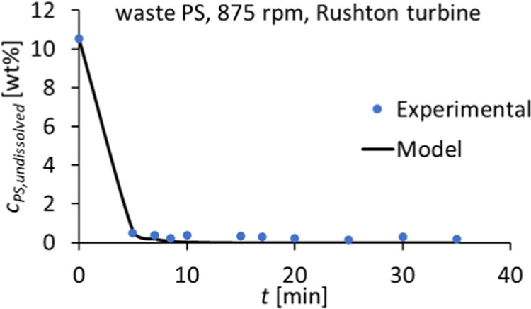
3.3. Case Study with Real Waste

The dissolution of a real PS waste sample in cyclohexene was studied in a baffled reactor. The waste sample consisted of foamed PS fish boxes that were compressed after collection at a sorting facility. Dissolution was performed at 50 °C and 875 rpm with particles in the range of 1.18–2.0 mm. The results show that full dissolution is obtained after 5 min, which is quite similar to the dissolution of pure PS at the same conditions (Figure 11). Despite the fact that the obtained EPS waste/cyclohexene had an unexpected yellowish color, the dissolution kinetics were not affected by the presence of these contaminants and/or additives.

Figure 11.

(a) Dissolution results for waste PS compared with pure PS and (b) dissolved waste in the reactor.

The kinetic model was also applied to the waste sample, which showed a very good fitting and a higher kinetic constant than the pure polystyrene dissolution, namely, of 0.56 min^–1 compared to 0.50 min^–1 for the pure PS at the same conditions (Figure 12). This may be related to the polymer (average) molar mass, which sometimes is lower for PS foams (M_w approximately at or above 200,000 g·mol^–1)⁵⁰ compared to that of pure GPPS for sheet extrusion (M_w typically above 250,000 g·mol^–1).⁵¹ Also, the low density may favor dissolution.

Figure 12.

First-order kinetic model (eq 2) fitting to experimental data of waste PS, K₁ = 0.56 min^–1.

4. Conclusions

In this work, a broad screening of promising solvents for polystyrene was performed, followed by the development of a multiple regression model to analyze the influence of solvent properties on the dissolution rate of polystyrene. The developed multiple regression model correlates with the experimental data with an adjusted R² of 0.9443, which is statistically significant. The results show that viscosity has the greatest influence on the dissolution of PS, followed by the individual Hansen solubility parameters, which describe the polarity of the solvent and thus the affinity for the solvent to the polymer. In future work, it would be interesting to apply and validate the model to other polymer–solvent systems.

Next, dissolution kinetic experiments were performed in a lab-scale reactor and a baffled reactor. The results indicate that a proper reactor design is able to decrease the dissolution time from 40 to 7 min. Furthermore, the impeller type plays an important role, and the results show that the Rushton turbine impeller performs very well with lower stirring velocities compared to the propeller-type impeller. The successful application of a first-order kinetics model confirmed that the dissolution in a baffled reactor is 5-fold faster than that in a lab-scale reactor, which again stresses the importance of a proper reactor design. It should be noted, however, that one of the limitations of a first-order kinetic model is that it is applicable only to a specific polymer–solvent system and cannot be extrapolated to other polymer–solvent systems. In future work, a more fundamental model would thus be relevant to understand and subdivide dissolution into diffusion and chain disentanglement phenomena.

Finally, the dissolution kinetics of a real PS waste sample from fish boxes were performed in the baffled reactor. After 5 min, dissolution was completed, which was confirmed by the first-order kinetic model. In summary, an increased dissolution rate is important for the industrial implementation of dissolution recycling of plastics, and this work shows which parameters mostly influence kinetics, including not only solvent properties but also proper reactor design.

Supporting Information Available

The Supporting Information is available free of charge at https://pubs.acs.org/doi/10.1021/acssuschemeng.3c08154.

• Reproducibility experiments results, correlation matrix, calibration curves, entanglement concentration determination, kinetic constants, and additional kinetic modeling results (PDF)

Author Contributions

R.K.: Conceptualization, methodology, software, validation, formal analysis, investigation, data curation, writing – original draft, and visualization; R.D.: conceptualization, methodology, software, writing – review & editing; G.B.: investigation, and validation, D.M.: investigation, writing – review & editing; E.B.-Z.: writing – review & editing; G.W.H.: formal analysis, writing – review & editing; N.N.: writing – review & editing; M.V.: writing – review & editing; A.L.: writing – review & editing; D.S.A.: writing – review & editing; S.D.M.: conceptualization, resources, writing – review & editing, supervision, project administration, and funding acquisition.

The authors declare no competing financial interest.

References

- Miller-Chou B. A.; Koenig J. L. A Review of Polymer Dissolution. Prog. Polym. Sci. 2003, 28 (8), 1223–1270. 10.1016/S0079-6700(03)00045-5. [DOI] [Google Scholar]
- Kol R.; De Somer T.; D’hooge D. R.; Knappich F.; Ragaert K.; Achilias D. S.; De Meester S. State-Of-The-Art Quantification of Polymer Solution Viscosity for Plastic Waste Recycling. ChemSusChem 2021, 14 (19), 4071–4102. 10.1002/cssc.202100876. [DOI] [PMC free article] [PubMed] [Google Scholar]
- Papanu J. S.; Soane Soong D. S.; Bell A. T.; Hess D. W. Transport Models for Swelling and Dissolution of Thin Polymer Films. J. Appl. Polym. Sci. 1989, 38 (5), 859–885. 10.1002/app.1989.070380509. [DOI] [Google Scholar]
- Peppas N. A.; Wu J. C.; von Meerwall E. D. Mathematical Modeling and Experimental Characterization of Polymer Dissolution. Macromolecules 1994, 27 (20), 5626–5638. 10.1021/ma00098a017. [DOI] [Google Scholar]
- Ghasemi M.; Singapati A. Y.; Tsianou M.; Alexandridis P. Dissolution of Semicrystalline Polymer Fibers: Numerical Modeling and Parametric Analysis. AIChE J. 2017, 63 (4), 1368–1383. 10.1002/aic.15615. [DOI] [Google Scholar]
- Marcon V.; van der Vegt N. F. A. How Does Low-Molecular-Weight Polystyrene Dissolve: Osmotic Swelling vs. Surface Dissolution. Soft Matter 2014, 10 (45), 9059–9064. 10.1039/C4SM01636J. [DOI] [PubMed] [Google Scholar]
- Mandema W.; Zeldenrust H. Diffusion of Polystyrene in Tetrahydrofuran. Polymer 1977, 18 (8), 835–839. 10.1016/0032-3861(77)90191-4. [DOI] [Google Scholar]
- Sánchez-Rivera K. L.; Munguía-López A. del C.; Zhou P.; Cecon V. S.; Yu J.; Nelson K.; Miller D.; Grey S.; Xu Z.; Bar-Ziv E.; Vorst K. L.; Curtzwiler G. W.; Van Lehn R. C.; Zavala V. M.; Huber G. W. Recycling of a Post-Industrial Printed Multilayer Plastic Film Containing Polyurethane Inks by Solvent-Targeted Recovery and Precipitation. Resour., Conserv. Recycl. 2023, 197, 107086 10.1016/j.resconrec.2023.107086. [DOI] [Google Scholar]
- Narasimhan B.; Peppas N. A. On the Importance of Chain Reptation in Models of Dissolution of Glassy Polymers. Macromolecules 1996, 29 (9), 3283–3291. 10.1021/ma951450s. [DOI] [Google Scholar]
- Valois P.; Verneuil E.; Lequeux F.; Talini L. Understanding the Role of Molar Mass and Stirring in Polymer Dissolution. Soft Matter 2016, 12 (39), 8143–8154. 10.1039/C6SM01206J. [DOI] [PubMed] [Google Scholar]
- Zhang Y.; Mallapragada S. K.; Narasimhan B. Dissolution of Waste Plastics in Biodiesel. Polym. Eng. Sci. 2010, 50 (5), 863–870. 10.1002/pen.21598. [DOI] [Google Scholar]
- Chen H.; Zhang E.; Dai X.; Yang W.; Liu X.; Qiu X.; Liu W.; Ji X. Influence of Solvent Solubility Parameter on the Power Law Exponents and Critical Concentrations of One Soluble Polyimide in Solution. J. Polym. Res. 2019, 26 (2), 39 10.1007/s10965-018-1694-0. [DOI] [Google Scholar]
- Kol R.; Nachtergaele P.; De Somer T.; D’hooge D. R.; Achilias D. S.; De Meester S. Toward More Universal Prediction of Polymer Solution Viscosity for Solvent-Based Recycling. Ind. Eng. Chem. Res. 2022, 61 (30), 10999–11011. 10.1021/acs.iecr.2c01487. [DOI] [PMC free article] [PubMed] [Google Scholar]
- Hansen C. M.Hansen Solubility Parameters: A User’s Handbook, 2007. [Google Scholar]
- EU Commission . Regulation (EC) No 1907/2006 of the European Parliament and of the Council of 18 December 2006 Concerning the Registration, Evaluation, Authorisation and Restriction of Chemicals (REACH), Establishing a European Chemicals Agency, Amending Directive 1999/45/EC and Repealing Council Regulation (EEC) No 793/93 and Commission Regulation (EC) No 1488/94 as Well as Council Directive 76/769/EEC and Commission Directives 91/155/EEC, 93/67/EEC, 93/105/EC and 2000/21/EC, 2006.
- Frisch M. J.; Trucks G. W.; Schlegel H. B.; Scuseria G. E.; Robb M. A.; Cheeseman J. R.; Scalmani G.; Barone V.; Petersson G. A.. et al. Gaussian 16, Rev. B.01.
- Becke A. D. Density-Functional Thermochemistry. III. The Role of Exact Exchange. J. Chem. Phys. 1993, 98 (7), 5648–5652. 10.1063/1.464913. [DOI] [Google Scholar]
- Lee C.; Yang W.; Parr R. G. Development of the Colle-Salvetti Correlation-Energy Formula into a Functional of the Electron Density. Phys. Rev. B 1988, 37 (2), 785–789. 10.1103/PhysRevB.37.785. [DOI] [PubMed] [Google Scholar]
- Tirado-Rives J.; Jorgensen W. L. Performance of B3LYP Density Functional Methods for a Large Set of Organic Molecules. J. Chem. Theory Comput. 2008, 4 (2), 297–306. 10.1021/ct700248k. [DOI] [PubMed] [Google Scholar]
- Kumari S. Multicollinearity: Estimation and Elimination. J. Contemp. Res. Manage. 2008, 3, 87–95. [Google Scholar]
- R Core Team . A Language and Environment for Statistical Computing, The R Project for Statistical Computing.
- Coker A.Fluid Mixing in Reactors. In Modeling of Chemical Kinetics and Reactor Design; Coker A. K., Ed.; Gulf Professional Publishing, 2001; pp 552–662. [Google Scholar]
- InstruLabo . InstruLabo.
- Doran P. M.Mixing. In Bioprocess Engineering Principles; Elsevier, 2012; pp 255–332. [Google Scholar]
- Gao Y.; Glennon B.; He Y.; Donnellan P. Dissolution Kinetics of a BCS Class II Active Pharmaceutical Ingredient: Diffusion-Based Model Validation and Prediction. ACS Omega 2021, 6 (12), 8056–8067. 10.1021/acsomega.0c05558. [DOI] [PMC free article] [PubMed] [Google Scholar]
- Costa P.; Sousa Lobo J. M. Modeling and Comparison of Dissolution Profiles. Eur. J. Pharm. Sci. 2001, 13 (2), 123–133. 10.1016/S0928-0987(01)00095-1. [DOI] [PubMed] [Google Scholar]
- Soetaert K.; Petzoldt T. Inverse Modelling, Sensitivity and Monte Carlo Analysis in R Using Package FME. J. Stat Software 2010, 33 (3), 1–28. 10.18637/jss.v033.i03. [DOI] [Google Scholar]
- Duda J. L.; Vrentas J. S.; Ju S. T.; Liu H. T. Prediction of Diffusion Coefficients for Polymer-Solvent Systems. AIChE J. 1982, 28 (2), 279–285. 10.1002/aic.690280217. [DOI] [Google Scholar]
- Taherzadeh M.; Haghbakhsh R.; Duarte A. R. C.; Raeissi S. Estimation of the Heat Capacities of Deep Eutectic Solvents. J. Mol. Liq. 2020, 307, 112940 10.1016/j.molliq.2020.112940. [DOI] [Google Scholar]
- Asmussen F.; Ueberreiter K. Velocity of Dissolution of Polymers. Part II. J. Polym. Sci. 1962, 57 (165), 199–208. 10.1002/pol.1962.1205716516. [DOI] [Google Scholar]
- Patterson D. Role of Free Volume Changes in Polymer Solution Thermodynamics. J. Polym. Sci., Part C: Polym. Symp. 1967, 16 (6), 3379–3389. 10.1002/polc.5070160632. [DOI] [Google Scholar]
- Saeki S.; Kuwahara N.; Nakata M.; Kaneko M. Upper and Lower Critical Solution Temperatures in Poly (Ethylene Glycol) Solutions. Polymer 1976, 17 (8), 685–689. 10.1016/0032-3861(76)90208-1. [DOI] [Google Scholar]
- Moldoveanu S.; David V.. Phase Transfer in Sample Preparation. In Modern Sample Preparation for Chromatography; Moldoveanu S.; David V., Eds.; Elsevier, 2021; pp 151–190. [Google Scholar]
- Ranade V. V.; Mashelkar R. A. Convective Diffusion from a Dissolving Polymeric Particle. AIChE J. 1995, 41 (3), 666–676. 10.1002/aic.690410323. [DOI] [Google Scholar]
- Ügdüler S.; De Somer T.; Van Geem K. M.; Roosen M.; Kulawig A.; Leineweber R.; De Meester S. Towards a Better Understanding of Delamination of Multilayer Flexible Packaging Films by Carboxylic Acids. ChemSusChem 2021, 14 (19), 4198–4213. 10.1002/cssc.202002877. [DOI] [PMC free article] [PubMed] [Google Scholar]
- Adebayo A. O.; Ipinmoroti K. O.; Ajayi O. O. Dissolution Kinetics of Chalcopyrite with Hydrogen Peroxide in Sulphuric Acid Medium. Chem. Biochem. Eng. Q. 2003, 17, 213–218. [Google Scholar]
- Baba A. A.; Adekola F. A.; Toye E. E.; Bale R. B. Dissolution Kinetics and Leaching of Rutile Ore in Hydrochloric Acid. J. Miner. Mater. Charact. Eng. 2009, 08, 787. 10.4236/jmmce.2009.810068. [DOI] [Google Scholar]
- Ismael M.; Mohammed H.; El Hussaini O.; El-Shahat M. Kinetics Study and Reaction Mechanism for Titanium Dissolution from Rutile Ores and Concentrates Using Sulfuric Acid Solutions. Physicochem. Probl. Miner. Process. 2021, 138–148. 10.37190/ppmp/145166. [DOI] [Google Scholar]
- Pekcan Ö.; Uĝur Ş.; Yılmaz Y. Real-Time Monitoring of Swelling and Dissolution of Poly(Methyl Methacrylate) Discs Using Fluorescence Probes. Polymer 1997, 38 (9), 2183–2189. 10.1016/S0032-3861(96)00769-0. [DOI] [Google Scholar]
- Kavanagh N.; Corrigan O. I. Swelling and Erosion Properties of Hydroxypropylmethylcellulose (Hypromellose) Matrices—Influence of Agitation Rate and Dissolution Medium Composition. Int. J. Pharm. 2004, 279 (1–2), 141–152. 10.1016/j.ijpharm.2004.04.016. [DOI] [PubMed] [Google Scholar]
- Reynolds T. D.; Gehrke S. H.; Ajaz S H.; Shenouda L. S. Polymer Erosion and Drug Release Characterization of Hydroxypropyl Methylcellulose Matrices. J. Pharm. Sci. 1998, 87 (9), 1115–1123. 10.1021/js980004q. [DOI] [PubMed] [Google Scholar]
- Asare-Addo K.; Kaialy W.; Levina M.; Rajabi-Siahboomi A.; Ghori M. U.; Supuk E.; Laity P. R.; Conway B. R.; Nokhodchi A. The Influence of Agitation Sequence and Ionic Strength on in Vitro Drug Release from Hypromellose (E4M and K4M) ER Matrices—The Use of the USP III Apparatus. Colloids Surf., B 2013, 104, 54–60. 10.1016/j.colsurfb.2012.11.020. [DOI] [PubMed] [Google Scholar]
- Asare-Addo K.; Levina M.; Rajabi-Siahboomi A. R.; Nokhodchi A. Study of Dissolution Hydrodynamic Conditions versus Drug Release from Hypromellose Matrices: The Influence of Agitation Sequence. Colloids Surf., B 2010, 81 (2), 452–460. 10.1016/j.colsurfb.2010.07.040. [DOI] [PubMed] [Google Scholar]
- Sedahmed G. Mass Transfer at the Impellers of Agitated Vessels in Relation to Their Flow-Induced Corrosion. Chem. Eng. J. 1998, 71 (1), 57–65. 10.1016/S1385-8947(98)00108-9. [DOI] [Google Scholar]
- Grisafi F.; Brucato A.; Caputo G.; Lima S.; Scargiali F. Modelling Particle Dissolution in Stirred Vessels. Chem. Eng. Res. Des. 2023, 195, 662–672. 10.1016/j.cherd.2023.06.026. [DOI] [Google Scholar]
- Green D.; Perry R.. Perry’s Chemical Engineers’ Handbook, 8th ed.; McGraw-Hill: New York, 2008. [Google Scholar]
- Askeland D. R.Lost Foam Casting (Disposable Mold). In Encyclopedia of Materials: Science and Technology; Jürgen Buschow K. H.; Cahn R. W.; Flemings M. C.; Ilschner B.; Kramer E. J.; Mahajan S.; Veyssière P., Eds.; Elsevier, 2001; pp 4641–4644. [Google Scholar]
- Wong C.-M.; Hung M.-L. Polystyrene Foams as Core Materials Used in Vacuum Insulation Panel. J. Cell. Plast. 2008, 44 (3), 239–259. 10.1177/0021955X08090420. [DOI] [Google Scholar]
Associated Data
This section collects any data citations, data availability statements, or supplementary materials included in this article.