Abstract
Tuberculosis (TB), primarily affecting the lungs, is caused by the bacterium Mycobacterium tuberculosis and poses a significant health risk. Detecting acid-fast bacilli (AFB) in stained samples is critical for TB diagnosis. Whole Slide (WS) Imaging allows for digitally examining these stained samples. However, current deep-learning approaches to analyzing large-sized whole slide images (WSIs) often employ patch-wise analysis, potentially missing the complex spatial patterns observed in the granuloma essential for accurate TB classification. To address this limitation, we propose an approach that models cell characteristics and interactions as a graph, capturing both cell-level information and the overall tissue micro-architecture. This method differs from the strategies in related cell graph-based works that rely on edge thresholds based on sparsity/density in cell graph construction, emphasizing a biologically informed threshold determination instead. We introduce a cell graph-based jumping knowledge neural network (CG-JKNN) that operates on the cell graphs where the edge thresholds are selected based on the length of the mycobacteria’s cords and the activated macrophage nucleus’s size to reflect the actual biological interactions observed in the tissue. The primary process involves training a Convolutional Neural Network (CNN) to segment AFBs and macrophage nuclei, followed by converting large (42831*41159 pixels) lung histology images into cell graphs where an activated macrophage nucleus/AFB represents each node within the graph and their interactions are denoted as edges. To enhance the interpretability of our model, we employ Integrated Gradients and Shapely Additive Explanations (SHAP). Our analysis incorporated a combination of 33 graph metrics and 20 cell morphology features. In terms of traditional machine learning models, Extreme Gradient Boosting (XGBoost) was the best performer, achieving an F1 score of 0.9813 and an Area under the Precision-Recall Curve (AUPRC) of 0.9848 on the test set. Among graph-based models, our CG-JKNN was the top performer, attaining an F1 score of 0.9549 and an AUPRC of 0.9846 on the held-out test set. The integration of graph-based and morphological features proved highly effective, with CG-JKNN and XGBoost showing promising results in classifying instances into AFB and activated macrophage nucleus. The features identified as significant by our models closely align with the criteria used by pathologists in practice, highlighting the clinical applicability of our approach. Future work will explore knowledge distillation techniques and graph-level classification into distinct TB progression categories.
Keywords: Acid-fast bacilli, cell graphs, convolutional neural network, granuloma, jumping knowledge neural network, pulmonary tuberculosis, whole slide image
I. INTRODUCTION
Tuberculosis (TB) is a contagious disease that is a significant cause of ill health and one of the leading causes of death worldwide. In 2022, it was diagnosed in 10.6 million human patients and resulted in 1.6 million deaths [1]. The infectious bacterium is the primary cause of pulmonary tuberculosis, which usually affects only the lungs after an airborne infection. Granulomas in the lung tissue are a defining feature of pulmonary TB in human and experimental animal models. The critical role of detecting acid-fast bacilli (AFB) in stained samples for TB diagnosis is a significant step in tuberculosis identification. WSI enables the digital examination of stained samples and allows for the analysis of tissues at a much higher resolution.
For many years, research on inbred laboratory mice has been instrumental in understanding the host reactions to Mycobacterium tuberculosis (M. tb), governed by individual cell types and genes. However, recently, researchers have focused on the introduction of genetically diverse animal models to pinpoint factors influencing lung damage from M.tb in immune-adequate hosts and the adoption of novel techniques to discover biomarkers in line with the World Health Organization’s (WHO) Target Product Profiles [2]. A new population of mice called Diversity Outbred (DO) mice, which has a level of genetic diversity comparable to that of humans is used in this study.
Currently, there are few known [3] automated algorithms that can identify specific, isolated cells within TB granulomas, such as specific AFB or specific activated macrophage nucleus. Several methods are in practice for TB diagnosis. These range from plain microscopic smears like Ziehl-Neelsen (ZN) stain to fluorescence smears such as auramine O and auramine-rhodamine stain. Molecular tests include transcription-mediated amplification, strand-displacement amplification, conventional PCR, and Xpert MTB/RIF. Other techniques include mycobacterial culture, drug susceptibility tests, histopathologic examinations, and immunologic tests like the tuberculin skin test (TST) and interferon-gamma releasing assay (IGRA) [4]. The ZN stained histopathological examination, recognized as the standard approach, is commonly adopted for diagnosing pulmonary TB because of its cost-effectiveness [5].
In digital pathology, deep learning techniques have been utilized to analyze WSI to predict lung and prostate cancer diagnoses and detect breast cancer metastases [6]. [7]. WSIs present a unique computational challenge due to their immense size, often exceeding one gigapixel. The predominant approach in deep learning for WSIs involves extracting a limited number of patches, typically ranging from 32 × 32 to 224*224, to manage the high dimensionality [8], [9], [10], [11], [12]. This selective input method is akin to manual feature selection and restricts the analysis to a fraction of the available data. Existing patch-based methods of WSI suffer from a trade-off between each image patch’s resolution and the available context. Working at higher resolutions enables the capture of finer cellular details, but it fails to capture the global tissue microenvironment. On the other hand, working at lower resolutions hinders access to cellular properties. Even if we could employ larger convolutional kernels to build Convolutional Neural Networks (CNNs) that handle larger images, the computational complexity of this operation would increase quadratically with the kernel size [13]. Another method known as a “bag of images” (a form of multi-instance learning) involves aggregating patch representations using autoregressive or attention-based methods to create a complete slide representation, disregarding regions outside of the tissue [14], [15], [16], [17]. However, they overlook crucial spatial relationships between patches by focusing on aggregated local features.
An emerging solution to fully leverage the rich information within WSIs is using cell graph representations that map the granuloma into a graph. However, existing methodologies [18], [19] for constructing cell graphs employ edge thresholding techniques, which can inadvertently discard vital biological information. This oversight may result in losing subtle yet crucial insights by producing overly sparse or dense graphs. Furthermore, the black-box nature of these models adds to the challenge by limiting interpretability, a critical aspect for domain experts who depend on transparent and actionable findings. Additionally, current approaches tend to simplify spatial interactions, ignoring the complexity of cellular interplay and thus compromising the predictive accuracy of the models.
The granuloma cell distribution is not random; instead, it is related to the underlying functional state. Cell graphs use graph features to mimic the interaction between different cells and the granuloma. We postulate that intricate spatial distribution information of the tissue environment is informative for predicting TB and that a graph neural network (GNN) model can efficiently utilize the functional patterns generated by cell graphs. A cell graph is constructed directly from the WSI, where the nucleus of activated macrophage and AFB are nodes, and graph edges are potential cellular interactions. The interactions are shaped using the biological context to provide a more informed representation. Our study introduces a Cell Graph Jumping Knowledge Neural Network (CG-JKNN) for node-level classification. To construct the feature set, we extract local and global graph-level attributes and neighborhood overlap features. Additionally, we derive the morphological features from the WSI without employing downsampling. Within our proposed graph model, we use the ideas of ‘jumping knowledge’ [20] from GraphSAGE layers. It gathers information from multiple network layers, not just the last one, allowing it to capture vital insights about each node. This jumping knowledge is then enhanced with GATv2’s attention mechanism, ensuring that the model pays the right amount of attention to the most informative nodes. We trained a set of ML algorithms, such as Random Forest [21], XGBoost [22], LightGBM [23], and Extra Trees [24], using our feature sets to assess their efficacy. Our proposed graph model’s performance was benchmarked against other graph models, including GraphSAGE with various aggregators [25] and Graph Attention Networks (GATv2 and GATConv) [26]. To better understand the decision-making process of our model, we utilized model interpretation methods like Shapely values and Integrated Gradients. The significance and logic behind these model interpretations were later interpreted with the help of the domain expert.
The major contributions of this work can be summarized as follows:
We introduced a novel approach to construct cell graphs by incorporating interaction threshold values based on the cord of mycobacterium and macrophage nucleus radius. This method enabled the creation of a biologically meaningful cell graph that accurately represented cell interactions.
To the best knowledge of the authors, this is the first study to utilize local and global neighborhood overlap features extracted from the cell graphs for TB detection.
A Graph neural network model with jumping knowledge that leveraged cell graphs, cell morphology features, and spatial information to achieve accurate node classification.
Conducted a thorough comparison of node classification performance between our graph-based and traditional machine learning (ML) models.
Conducted four ablation studies, focusing on diverse node aggregation techniques, combinations of features, the impact of jumping knowledge, and the impact of random weight initialization along with different data subsets.
Employed model interpretation techniques, including Shapely additive explanation (SHAP) [27] and Integrated Gradients [28], to gain insights into the model’s decision-making process and collaborated closely with domain experts to analyze the significance and rationale behind these interpretations.
The rest of the paper is organized as follows: Section II explains the related works. The methodology of the proposed work is described in Section III. The evaluation criteria are shown in Section IV. Section V represents the classification results of the study. The results of model interpretation are shown in Section VI. The results of the XGBoost with top K features are presented under section VII. The ablation studies are shown in the Section VIII. Section IX presents the work’s conclusion and future directions.
II. RELATED WORKS
Characterization of TB in Animal Models:
In tuberculosis research, using mice and other rodents has provided helpful information about the host’s susceptibility to M.tb infection. This knowledge has been used to know the pathological pathway of the bacteria once it infects a host and to create perfect tools for diagnosing, treating, and preventing tuberculosis [5]. Mice are commonly chosen as model animals for several practical reasons. These include the ready availability of immunological tools specifically designed for mice, the presence of genetically modified mouse strains that enable targeted research, and the convenient attributes of mice, such as their compact size and cost-effective maintenance in laboratory settings [29], [30], [31], [32]. In the literature, works involved designing a histological categorization system to assess the advancement of pulmonary lesions in TB animal models. This system involved evaluating granulomatus lesions and assigning numerical categories based on the number of inflammatory cells present and the pattern of their infiltration within the tissue [33]. In [2], they infected DO mice with aerosolized M.tb, resulting in a range of human-like phenotypes. After examining gene expression and immune responses, they measured 11 proteins in 482 mice (453 infected, 29 non-infected). Two mouse lung biomarkers were chosen through exhaustive testing of various classification algorithms and biomarker combinations. Their effectiveness in diagnosing active TB was tested on human samples from the Foundation for Innovative New Diagnostics. Deep learning methods have recently gained widespread adoption in this field, revolutionizing the analysis of pulmonary tissues in the tuberculosis mouse model. CNNs were utilized in [34] to classify seven distinct pathology features found in pulmonary tissues of the C3HeB/FeJ tuberculosis mouse model. In [35], the authors employed Attention-based deep learning to identify and quantify histopathology-based biomarkers in M.tb infected DO mice lung tissue samples. Unlike human pathologists, the model could accurately measure these features, making it a powerful tool for statistical analysis. The authors in [36] presented a novel approach that predicted specific gene expression values using histopathological images, serving as an intermediary step to detect ‘supersusceptible’ pulmonary tuberculosis in DO mice subjected to experimental infection.
Cell Graphs:
Cell graphs are a representation of the interactions between cells in the tissue. They are built by transforming tissue images into a graph structure, where each node represents a single cell, and the connections between nodes reflect possible interactions between cells. Adding incorrect information to graph formulations could harm the training process, highlighting the necessity for thorough examination [37]. The cell graph can be analyzed using various graph theoretical methods to extract information about the organization and behavior of cells in the tissue. This can be used to gain insights into cell behavior and aid in understanding biological processes.
Graph edges are configured to denote the potential cellular interactions. It is assumed that nearby cells are more likely to interact with one another. Researchers frequently construct graphs using Delaunay triangulation [38], [39] or the K-nearest-neighbor (KNN) approach [18], [19], [40], [41] to depict these interconnections. The Waxman model [42] is another alternative strategy that uses exponential decay based on Euclidean distance to represent cell interactions.
Based on the spatial proximity of the cells, edges are formed between individual cells or cell clusters that create a Delaunay triangle in the Delaunay triangulation technique. On the other hand, the K-nearest-neighbor technique links each cell or cluster to its K-nearest neighbors, highlighting the local cell-cell relationships. Cell graphs have applications in various biology and biomedical research tasks, from modeling bone tissue to predicting cancer and estimating distant metastasis. In [43], the authors combined the ECM formation with the distribution of cells in hematoxylin and eosin (H&E) stained histopathological images of bone tissue samples to achieve bone tissue modeling and classification. Cell graphs offer insights into the heterogeneity and complexity of the tumor microenvironment (TME), aiding in cancer staging. A hierarchical Transformer Graph Neural Network trained on cell graphs was employed for the colorectal adenocarcinoma grading task in [41], and a novel cell-graph convolutional neural network was employed for colorectal cancer grading in [40]. Graphs featuring 1000-3000 cells with 2000-10,000 links determined by spatial proximity enabled the distinction between cancerous, healthy, and inflamed cells in brain cancer tissue [44]. CGSignature, an AI-powered graph neural network approach utilizing spatial TME patterns from mIHC images to stage TME and digitally predict patient survival in gastric cancer, was proposed in [45]. All the abovementioned methods used simple spatial information, global graph-level features, or morphology features for further classification or clustering. In [37], the authors introduced a framework combining the global image-level insights obtained from CNNs with the cell-level spatial geometry captured by GNNs, enhancing overall image representation. They chose the edge threshold based on the tissue structure, image category, and magnification of the WSI. Augmented cell graphs with multilayer perceptron (MLP) were employed to classify brain cancer samples in [46]. Cell clusters were utilized as nodes in the cell cluster graph (CCG) constructed in [47]. Edges in the CCG were established using a decaying probability function with an exponent of −α. In [48], the authors introduced the Feature Driven Local Cell Graph (FeDeG) for constructing cell graphs from H&E stained tissue images and derived predictive metrics to train a linear discriminant classifier to predict lung cancer survival. A hierarchical cell-to-tissue-graph (HACT) model was developed in [49] that, compared to existing models, closely resembled pathological diagnostic procedures and captured both cellular interactions and tissue morphology for detecting breast cancer. By positioning nodes in Euclidean space and linking them with edges where the likelihood of a link exponentially decays with their Euclidean distance, the Waxman model proposed in [42] created a cell graph that reflected the incidence of cancer or disease-related traits.
Graph Neural Network With Cell Graphs for Disease Prediction/Classification:
There have been recent advancements in using GNN to learn patterns from the TME [40]. The detailed spatial distribution within the TME holds valuable information that plays a vital role in predicting diseases. A GNN model can understand the intricate patterns in cell graphs, turning them into valuable insights for diagnosis and prognosis. In [45], the authors constructed and compared four distinct GNN model architectures: GCNSag, GCNTopK, GINSag, and GINTopK to achieve accurate prediction of patient survival in gastric cancer. Adaptive GraphSAGE was employed in [40] to dynamically merge multi-scale graph features to classify colorectal cancer cases. In [50], the authors utilized a Graph Convolutional Network combined with Jumping Knowledge and GraphSAGE to distinguish between Dysplastic and normal intestinal glands. They explored various message-passing neural network variants, contrasting them with a traditional graph method using approximated graph edit distance and a K-nearest neighbors classifier. The authors in [41] introduced a hierarchical network to achieve the grading of colorectal cancer images. It integrated the GIN module with the Min-CutPool module for enhanced graph differentiation. Additionally, a Transformer module was incorporated to capture long-distance dependencies. The authors in [19] introduced the CGAT network for precisely classifying pancreatic cancer and its precursors from immunofluorescence histology images. It integrated a unique self-attention mechanism at its output, enhancing interactions among graph nodes. This mechanism assigned weights to node embeddings, with higher-weighted nodes playing a more significant role in model predictions.
In existing studies, cell graph construction lacked biological context, often prioritizing proximity-based interactions or striving for a balance between connected-only and complete graphs. Additionally, they either focused on simple spatial metrics such as the X and Y coordinates of the cell (center of the cell) or the morphology of the cells. Furthermore, they used the same settings across different models and did not fine-tune the model’s hyperparameters for each feature set.
CT and X-Ray Imaging in Tuberculosis Diagnosis:
In [51], the authors proposed a 3D-ResNet framework based on Computed Tomography (CT) Scan images to differentiate nontuberculous mycobacterium lung disease (NTM-LD) from mycobacterium tuberculosis lung disease (MTB-LD). Using data from 301 NTM-LD and 804 MTB-LD patients, the model achieved AUCs of 0.90, 0.88, and 0.86 in training, validation, and testing, respectively, and 0.78 on an external test set. The study concluded that 3D-ResNet, significantly outperforming radiologists in detecting lung abnormalities, was an effective rapid diagnostic tool for NTM-LD and MTB-LD, offering the potential for improving treatment strategies. In [52], they introduced Healthcare-As-A-Service (HAAS), a novel cloud-based lung cancer diagnosis service utilizing HAASNet, a CNN with a 96.07% accuracy rate. Integrating cloud technology and the Internet of Medical Things, HAAS offered accurate, globally accessible lung cancer diagnostics, achieving precision, recall, and F1-scores of 96.47%, 95.39%, and 94.81%, respectively. In [53], the authors introduced a depth-enhanced 3D block-based ResNet (depth-ResNet) for classifying the severity of TB from CT pulmonary images, addressing challenges in small datasets and localized abnormalities. The depth-ResNet demonstrated superior performance with a 92.70% accuracy in predicting TB severity scores, outperforming the standard ResNet-50. It also effectively assessed high severity probabilities, achieving average accuracies of 75.88% and 85.29% using innovative probability-based severity measures.
LungNet, a novel hybrid deep-convolutional neural network model that leveraged CT scans and medical IoT data to diagnose lung cancer accurately, was proposed in [54]. With its unique 22-layer CNN architecture, LungNet achieved a high accuracy of 96.81% and a low false positive rate of 3.35%, efficiently classifying lung cancer into five classes and further into sub-stages 1A, 1B, 2A, and 2B with 91.6% accuracy. This advanced diagnostic capability positioned LungNet as a significant advancement in automatic lung cancer detection systems. In [55], a multiclass lung disease classification using a fine-tuned CNN model was proposed to identify ten different lung diseases from chest X-rays, including COVID-19, Tuberculosis, and Pneumonia. Initially employing eight pre-trained models like VGG16 and ResNet50, the VGG16 was then enhanced into LungNet22, a customized model achieved by adding several layers to the VGG16 model. This model achieved a notable accuracy of 98.89%. This approach, validated through performance metrics like ROC curves and AUC values, marked a significant step in efficient, reliable lung disease diagnosis using X-ray imaging. The works discussed here utilize CT scan and X-ray images for diagnosing lung diseases. CT scans are invaluable for identifying granulomas’ location, size, and spread. However, CT scans and X-rays, while effective for macroscopic analysis, do not allow for direct observation of tissues at the cellular level, such as individual cells or bacteria. This limitation is due to the nature of CT imaging and X-rays, which are not designed for cellular-level detail, unlike WSI, which offers rich microscopic information.
The summary of the works that use cell graphs for disease classification is tabulated in Table 2.
TABLE 2.
Related works.
| Model | Dataset | Performance | Ref |
|---|---|---|---|
| GraphSAGE-mean | Placenta Histology Data | Accuracy: 88.94 ±0.38 | [56] |
| MLP and Transformer | CRC-MSI, STAD-MSI, and GIST-PDL1 | AUC improvement of more than 5% on various network backbones | [37] |
| Adaptive GraphSAGE with Graph Clustering module | Colorectal Cancer Data | Patch Accuracy : 91.60 ± 1.26, Image Accuracy: 97.00 ± 1.10 % | [40] |
| Hierarchical Transformer Graph Neural Network | Colorectal Cancer Dataset (CRC) and Extended Colorectal cancer dataset (Extended CRC) | Accuracy on CRC:98.55±1.26 %, Accuracy on Extended CRC : 95.33±0.58 % | [41] |
| GINConv+TopKPool | Gastric Cancer | AUC of Binary classification: 0.960±0.01, AUC of Ternary classification: 0.904±0.012 | [45] |
| Cell-Graph Attention (CGAT) network | Pancreatic Diseases and Cancer | Precision: 0.73, Recall:0.65 and F1-score:0.62 | [19] |
| Augmented Cell Graph and MLP | Brain Cancer | Sensitivity: 97.53% and Specificities of inflamed and healthy: 93.33% and 98.15% | [46] |
| Extracellular matrix (ECM)-aware cell-graph with Support Vector Machine (SVM) | Bone Cancer | Accuracy: 90% | [43] |
| Hierarchical Cell-to-Tissue (HACT) network | Breast Carcinoma Subtyping Set | Weighted F1 score : 61.53±0.87 | [49] |
| Feature Driven Local Cell Graph with linear discriminant classifier | Lung Cancer | AUC = 0.68 | [48] |
| Cell Cluster Graph with SVM | Prostrate Cancer | Accuracy : 83.1 ±1.2% | [47] |
| Hierarchical Cell Graphs and SVM | Breast Cancer | Accuracy :81.8% | [18] |
III. METHOD
The workflow of the proposed study is presented in figure 1.
FIGURE 1.
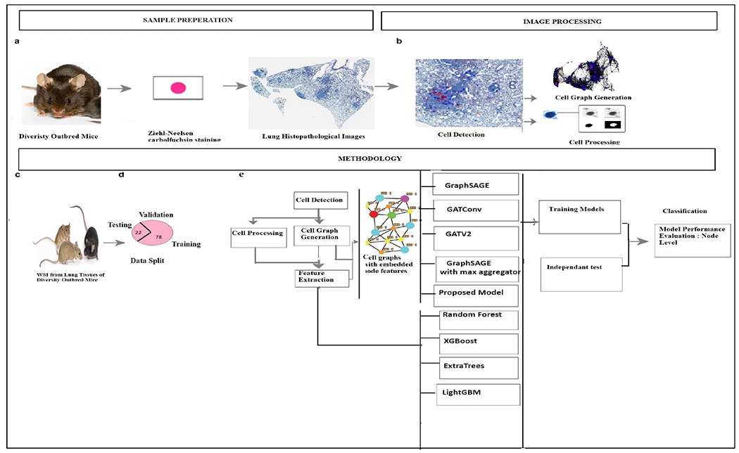
Overall Workflow: (a). Specimen processing: Extract lung tissues from DO mice and stain them with Ziehl-Neelsen stain. (b). Detect cells, construct cell graphs, and process them. (c). A total of 44 cases are considered (Images of mice in this figure are adapted from The Jackson Laboratory (2023). Retrieved from https://www.jax.org/strain/009376). (d). Split of Data. (e). Overall Methodolog.
A. DATASET
Eight-week-old female DO mice, sourced from The Jackson Laboratory in Bar Harbor, ME, were accommodated in a Biosafety Level 3 facility at the New England Regional Biosafety Laboratory, part of Tufts University’s Cummings School of Veterinary Medicine in North Grafton, MA. These mice underwent an infection process, exposing them to 20-100 Colony Forming Units of M.tb Erdman, utilizing the CH Technologies nose-only exposure technique, as cited in prior studies [57], [58]. WSI was then generated from these stained lung tissue samples for further analysis in our proposed method.
For this work, we used 44 WSI with an average size of 42831*41159 at 40X magnification. The cells in the images are divided into AFB and the nucleus of activated macrophage. The dataset was split into training, validation, and test sets, with 34 WSI in the training and validation set and 10 in the test set. Given that the focus of the study was primarily on infected samples, only two were uninfected, with the majority being infected. This resulted in more AFBs than the nucleus of activated macrophages, leading to an imbalanced dataset. Sample images from the dataset are shown in figure 2.
FIGURE 2.
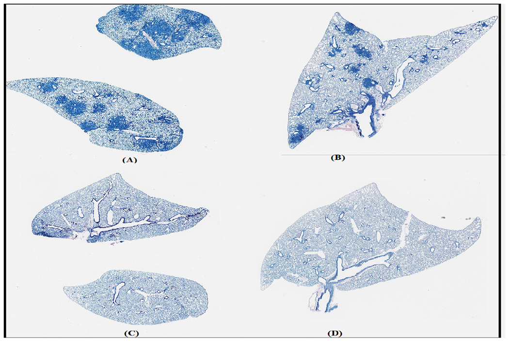
Sample images. (A) and (B). TB infected. (C) and (D). Uninfected.
B. DETECTION AND SEGMENTATION OF NUCLEUS OF ACTIVATED MACROPHAGES AND AFB
The detection of M.tb, which stains positive using the modified Ziehl-Neelsen method, plays a crucial role in diagnosing tuberculosis. Activated macrophages are a vital component of the immune response to infection. A two-layer CNN was developed to detect these two types of cells using Aiforia Cloud version 5.1.1 from Aiforia Technologies in Helsinki, Finland. The main advantage of using this platform is that the researchers can focus on data annotating and improving AI models’ performance without worrying about fine-tuning hyperparameters. The model was trained on WSI from experimental mouse tuberculosis infections.
The training set consisted of 18 whole slide images from the lungs of DO mice, C57BL/6J mice, and BALB/c mice [59]. The first layer was trained to segment the tissue in the WSI, while the second layer was trained to classify three different types of objects within the segmented tissue layer: individual AFB, clusters of AFBs, and nuclei of activated macrophages. The training images were manually annotated by a second-year veterinary student (Diana Choi, DC) under the supervision of a board-certified veterinary pathologist (Gillian Beamer, GB). The individual and cluster of AFBs were recognized by their dark red color, small size in longitudinal, oblique, or cross-sectional profiles, and intracellular or extracellular location. The macrophage nucleus was recognized by its relatively large size, “open-faced” appearance, and abundant cytoplasm. AFBs were annotated using an object diameter of 5μm and the nucleus of activated macrophage was annotated using an object diameter of 10μm. In this two-layered training approach, the first layer is designed to identify and remove non-relevant elements, such as artifacts and white spaces, from the images. The second layer is specifically trained to focus on distinguishing and excluding histological features that are neither acid-fast bacilli (AFBs) nor the nuclei of activated macrophages. The model was tested on 160 WSI. The error rate was used as a performance metric to evaluate the accuracy of the model’s predictions. The algorithm successfully detected lung tissue, the nucleus of activated macrophage, and AFBs with error rates of 3.09%, 2.27 %, and 9.05% (when compared with ground truth annotations). Figure 3 displays a heatmap of the regions segmented, while Figure 4 illustrates an example of a false positive result produced. In the rest of this article, the term ‘nuclei’ is used to refer to the nucleus of an activated macrophage.
FIGURE 3.
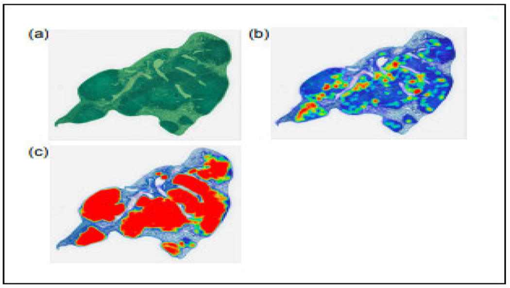
(a) Green region indicates model detection of lung tissue from a whole slide image. (b) The heat map shows activated macrophage nuclei detected by the model. (c) The heat map shows AFB detected by the model. The heat maps demonstrate the location and spatial information of AFB and activated macrophage nuclei within lung tissue.
FIGURE 4.
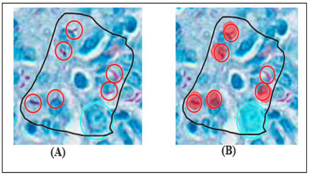
Verification of model training: example of a false negative result. (A) A human annotation of 6 single AFBs (red open circles) and 1 normal nucleus (blue open circle) within the training region. (b) The AI model detected 5 AFBs and one nucleus. The filled in circles indicate successful detection, true positives. The red open circle indicates where the model did not detect.
1). PROCESSING OF AFB AND NUCLEUS FOR MORPHOLOGICAL FEATURE EXTRACTION
The OpenSlide library [60] facilitated direct access to the high-resolution SVS files (WSI) without downsampling. The AFB and nucleus of activated macrophage were extracted with dimensions (40 × 40) centered around specific coordinates in the input image provided by our model and then converted to grayscale. The bounding box dimensions were chosen based on the object detector size used in the cell detection stage. A series of morphological operations, including top-hat and black-hat transforms with structuring elements of size (3,3), were applied to enhance the grayscale image. A threshold value obtained using global Otsu’s threshold was used to convert the image to binary. Post-processing was considered in the proposed method to get an accurate region of interest. Morphological opening and erosion using an ellipse-shaped structuring element of size (1,1) were performed to remove noise and imperfections from the binary image [61].
The hole-filling operation was performed as it helps to complete regions that might have been missed during the previous processing steps. The distance transform was computed using “ndi.distance_transform_edt()”. Peak local maxima within this distance-transformed image were detected using “peak_local_max().”The identified peak maxima were used to generate a marker image by applying the “ndi.label()” [62] function, which assigns unique labels to each detected maximum. Watershed segmentation was then performed on the distance-transformed image using the marker image as the input. This segmentation technique effectively separated overlapping objects and defined their clear boundaries. The processing quality was validated in collaboration with a domain expert, who assessed the results using a representative sample of images. The final image with the region of interest was considered for morphological feature extraction. The cell processing stages are shown in Figure 5.
FIGURE 5.
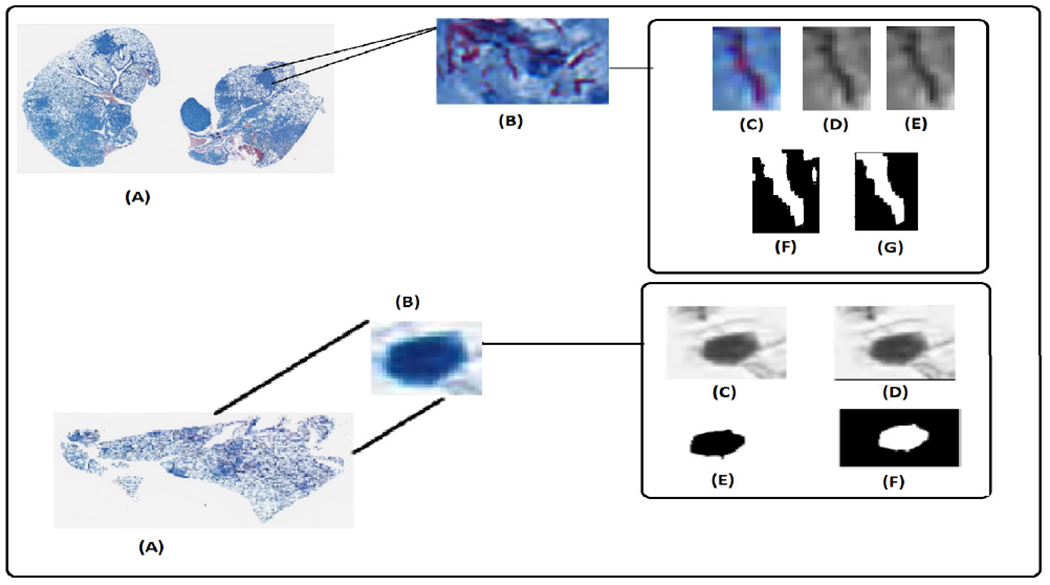
Upper Row: (A). Original Image. (B). Region of Granuloma with AFB. (C). Single AFB at the location (pixel) (46200,12954)in the original image. (D). Grayscale image. (E). Enhanced image. (F). Binary image before post-processing. (G). AFB. Lower Row: (A). Original Image. (B). Activated macrophage nucleus at the location (pixel) (25424,16909) in the original image. (C). Grayscale image. (D). Enhanced image. (E). Image after morphological operations. (F). Nucleus.
C. CONSTRUCTION OF THE CELL GRAPH
The threshold (edge threshold) for intercellular communication plays a pivotal role in cellular studies, and many studies have been conducted to determine the effective distance threshold for intercellular communication. The inputs from pathologists can offer valuable insights for improving the graph representation, ensuring it accurately reflects the biological relationships between the cells [50].
Euclidean distance as a proximity measure is a common approach in image analysis. A threshold distance of 20 micrometers between cell-cell pairs was used in [45]. Any cell-cell pairs closer than this distance would be connected by an edge in the graph. A fixed distance was used in [40] to assign an edge between two nuclei. Each node’s maximum degree was also set to k, the number of its k-nearest neighbors. Graphs with three different edge thresholds, 60, 75, and 90μm, were constructed and tested to identify the suitable threshold value in [63]. The threshold value 75μm resulted in a densely connected graph and was finally opted. The likelihood of nodes being connected decreased as a function of the distance in [64]. The probability of two cells being linked (i.e., being grown from the same parent cell) was related to the distance between them. The closer the cells were to each other, the more likely they were linked. A slightly different approach was employed in [18] where a hierarchical graph was formed by first identifying individual cells in the breast tissue image, and a grid was used to divide the image into smaller regions. The probability that each region is a cluster (lobe) of cells was calculated by dividing the number of cells in the region by the region’s size. A threshold value was set, and regions with a probability more significant than this threshold were considered clusters. In [65], the threshold values were chosen based on nucleus-membrane ratio and cell diameter. A 10-fold cross-validation approach was employed to identify the threshold value between the cells in the bone tissue modeling [43]. The threshold ranging from 20 to 60 pixels with increments of 5 pixels was selected that determined the sparsity or density of the resulting graphs. Lower thresholds resulted in sparser graphs, and higher thresholds resulted in denser graphs with more distant nodes being connected [66]. In [37], the authors chose the edge threshold based on the tissue structure, image category, and magnification of the WSI. A dataset was developed to forecast microanatomical tissue structures using cell graphs derived from placenta histology whole slide images in [56]. The authors of this paper constructed the intersection graph by combining two edge-building algorithms, KNN, and Delaunay Triangulation, using a value of k=5. A cell graph was generated in [42] using the Waxman model with edges where the probability of a link exponentially decayed with their Euclidean distance.
The cords of the M.tb infected cells are very long, reaching a length of up to 150 micrometers after 72 hours of infection [67]. Unlike the nucleus of activated macrophages, which are typically spherical, AFBs exhibit a distinct shape. This non-spherical morphology facilitates more significant detection as the macrophages extend pseudopods to sense their environment [68]. The position of the cells in the tissue affected by M.tb determines which cells will interact with each other. Cells can extend part of their body (pseudopods) beyond their normal boundary (radius) to detect other cells that are farther away, allowing the detection range to exceed the standard limit of the cell’s radius [68].
We hypothesize that AFBs can interact with other AFBs within 150 μm [67]. It is equivalent to 615 pixels in the magnification of this study. The nucleus of activated macrophages can interact among themselves and other AFBs if they are at a distance of 200 times [68] their radius, which comes up to 500 μm. It is equivalent to 2049 pixels in the magnification of this study. These threshold values have also been reviewed and approved by our domain expert. As a result of these interactions, the cell graphs in our study exhibited an average of 3.2k nodes per graph. This number was comparable to the number of nodes per graph reported in [40]. The adjacency matrix can be computed as follows:
Distance denotes Euclidean distance computing using the equation 1. The coordinates (xu, yu) belongs to node ‘u’ and the coordinates (xv, yv) belons to node ‘v’ in the image.
| (1) |
The distance threshold values chosen are tabulated in the table 3.
TABLE 3.
Distance thresholds.
| Node ’u’ | Node ’v’ | Distance ’d’ in pixels |
|---|---|---|
| AFB | AFB | 615 |
| AFB | Nucleus | 2049 |
| Nucleus | AFB | 2049 |
| Nucleus | Nucleus | 2049 |
Figure 6, (A) shows the cell graph of an uninfected case. (B) shows the cell graph of an infected case. The density of cell interactions is observed to be higher in cases of infection. This can be attributed to the presence of granulomas in the infected lung tissues, which are absent in uninfected lung tissue samples. This difference in the number of cell interactions between the two cases can be used as a diagnostic marker for infection or disease progression, and it also provides insight into the underlying mechanisms of the disease. Figure 7 presents the cell graphs overlaid on the WSI.
FIGURE 6.
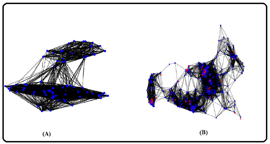
Blue nodes indicate nucleus of activated macrophage. Red nodes denoted AFB. Black lines (edges) denote the interactions between the nodes. (A). Cell graph of an uninfected sample. (B). Cell graph of an infected sample.
FIGURE 7.
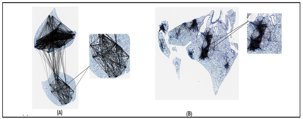
Typical cell graphs from (A) Uninfected Sample (B) Infected Sample.
D. ARCHITECTURE OF CELL GRAPH NETWORK
A graph is defined as G = (V, E), where V denotes the set of nodes. Each node v is associated with a d-dimensional feature vector . Edges are denoted as E where eu,v = (u, v) ∈ E signifies the presence of an edge between nodes u and v. The adjacency matrix represents the graph. Let denote the hidden features of node v in the l-th layer of a neural network. We initialize the input layer as , meaning the initial hidden features in the network equal the node features for the input layer.
In the proposed CG-JKNN, we use GraphSAGE to learn the nodes’ hidden representation. Each GraphSAGE layer processes the predefined aggregation function (in this case, ‘mean’ aggregation) to gather information from neighboring nodes. The mean aggregation computes the average of neighboring node representations. After processing through each layer with mean aggregation, the model combines the multi-level node representations by concatenating them. The neighborhood aggregation step is written as eq. 2 and combining step is demonstrated in eq. 3.
| (2) |
where represents the aggregated representation of the neighborhood N(v) for node v at layer l. represents the representation of neighboring node u at the previous layer (l − 1).
| (3) |
where represents the updated representation of node v at layer l. represents the aggregated neighborhood representation for node v at layer l, which was computed in the neighborhood aggregation step. W represents a learnable weight matrix that is applied to the concatenated representations of and .
The “jumping knowledge representation learning” was introduced in [20]. This approach allows a model to aggregate information from all hidden layers, not just the final layer. This can lead to a more comprehensive node representation that captures local and global graph structures. The authors in [20] experimented with three aggregation mechanisms: concatenation, max-pooling, and an LSTM-attention mechanism.
We incorporate a concatenation-based jumping knowledge mechanism into our network. Figure 8 depicts the overall architecture, and Figure 9 illustrates the concept of the jumping knowledge. Like typical neighborhood aggregation networks, each layer expands the range of influence by gathering information from neighborhoods in the previous layer [20]. At the last layer, for each node, we select all the intermediate representations from layers 1 to layer l-1 (total ‘l’ layers) representations which “jump” to the last layer. The total number of layers varies based on the feature set. The final hidden representation of a node is obtained by concatenating its hidden representations from each GraphSAGE layer. Specifically, after each layer, we store the intermediate node representations. At the end of the network’s forward pass, these stored representations for a specific node from all layers are concatenated to produce the node’s comprehensive and final hidden representation. Eq 4 represents the concatenation. This aggregation mechanism optimizes the weights to combine subgraph features in a manner that is most suitable for the dataset as a whole rather than being node-adaptive. We do not incorporate the max readout operation [40], [41] used for graph-level classification tasks, as our focus is on node-level classification. After obtaining the hidden representation through concatenation, these concatenated features are then fed into the GATv2 layer [69]. This layer further refines the node representations by leveraging attention mechanisms.
| (4) |
FIGURE 8.

Overview of the CG-JKNN.
FIGURE 9.
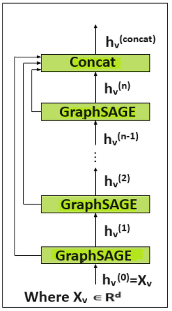
Jumping knowledge architecture.
As shown in eq. 5, for a node v and its neighboring node u, the attention mechanism can be expressed to capture the importance of node u to node v.
| (5) |
Here, a is the attention mechanism’s weight vector, and W is a weight matrix transforming the concatenated node representations. The updated node representation is obtained using eq.6.
| (6) |
where denotes the neighbors of node v, and σ is the activation function. We use a rectified linear unit (ReLU) as the activation function. We finally apply the softmax function to the output to obtain the node-level predictions.
Over-Smoothing Problem:
Over-smoothing has been consistently identified as a significant challenge in the GNNs, as reported in numerous works in the existing literature [40], [70], [71], [72], [73], [74]. Over-smoothing occurs when deep graph convolutional networks utilize too many layers, causing nodes to lose their original input characteristics and making training difficult.
Several techniques exist aimed at mitigating over-smoothing issues in GNNs. Energetic Graph Neural Networks introduce energy-based modeling [75], while Graph DropConnect adds graph-specific dropout [76].
Graph-coupled oscillator Networks use non-linear oscillators coupled through the graph to change GNN dynamics [77]. Additionally, adding residual connections in deep GNNs aids information flow and mitigates oversmoothing [78]. The DropEdge approach employed in this study addresses both issues by selectively removing edges during training, enhancing model performance, and avoiding over-smoothing. It also consistently leads to performance improvements in various GCNs, whether they are shallow or deep [79]. During each training epoch, the DropEdge technique simulates edge dropout in the input graph by randomly removing a proportion ‘p’ of edges from the adjacency matrix [79]. ‘A_drop’ signifies the resulting matrix, ‘A’ is the original matrix, and ‘A0’ is a primarily empty matrix with some extra connections randomly chosen from the initial set of connections represented by ‘E’. ‘Vp’ denotes the number of additional connections selected randomly from ‘E’ to expand the sparse matrix ‘A0’. The approach is as follows:
| (7) |
V is the total number of edges, and p is the dropping rate. We conducted experiments using a range of probability values, spanning from 0.1 to 0.9, and finally chose p = 0.1 for our overall experiment. In the proposed work, we utilize the edge index representation to represent the connections in the graph.
E. FEATURE EXTRACTION
GNN is a deep learning model designed explicitly for graph-structured data. It can effectively capture the complex relationships between nodes in a graph and learn valuable representations that can be used for various graph-related tasks. Many research papers [18], [40], [43], [45], [50], [64] in this domain have focused on using morphological features or graph features or simple spatial information. In contrast, our paper takes a unique approach by not only extracting a wide range of graph-based features (including both local and global neighborhood overlap metrics) but also incorporating various morphological features. The neighborhood overlap features prove valuable as they address the gap created by the limitations of node and graph level features in capturing relationships between neighboring nodes [80]. Table 4 and 5 list the features and descriptions. The features are scaled using the standard scaler (due to the wide variation between feature values) before training the graph-based models. It helps to ensure that all features are on a similar scale and can help reduce outliers’ impact [81]. There is an argument that handcrafted features are less effective than learned features, such as CNN features, and CNN-based methods can obtain more comprehensive morphological information [41]. Given the limited size of our dataset, we decided to utilize handcrafted morphology features.
TABLE 4.
Graph features.
| Feature | Description | Feature | Description |
|---|---|---|---|
|
| |||
| Number_of_nodes | The number of nodes in the graph . | Eigen_one_L | Number of eigenvalues of Laplacian matrix that have a value of one . |
| Number_of_edges | The number of edges in the graphs (interaction between the nodes). | Eigen_two_L | Number of eigenvalues of Laplacian matrix that have a value of two . |
| Eccentricity | The maximum graph distance between a vertex v and any other vertex u in a connected graph G . | Lower_slope_L | Line segment’s slope that corresponds to Laplacian matrix’s eigenvalues between 0 and 1. |
| Diameter | Maximum eccentricity. | Upper_Slope_L | Line segment’s slope that corresponds to Laplacian matrix’s eigenvalues between 1 and 2. |
| Radius | Minimum eccentricity. | Lower_slope_A | Line segment’s slope that corresponds to adjacency matrix’s eigenvalues between 0 and 1. |
| Center | The group of nodes having an eccentricity equal to the radius. | Upper_slope_A | Line segment’s slope that corresponds to adjacency matrix’s eigenvalues between 1 and 2 |
| Closeness_of_node | Denotes node’s proximity to all other nodes in the network. | Eigen_zero_A | Number of eigenvalues of adjacency matrix that have a value of zero. |
| Average_clustering | Mean of local clustering of the graph. | Eigen_one_A | Number of eigenvalues of adjacency matrix that have a value of one. |
| Node_clustering | Degree to which nodes in a graph tend to cluster together. | Eigen_two_A | Number of eigenvalues of adjacency matrix that have a value of two. |
| Trace_A | Sum of the diagonal elements of the adjacency matrix from upper left to lower right. | Sorenson | Ratio of nodes u and v’s common neighbors to their average node degrees. |
| Energy_A | Sum of absolute value of adjacency matrix’s eigenvalues . | Salton | Angle between columns of the adjacency matrix corresponding to the specified vertices, expressed as a cosine. |
| Connected_ratio | Number of nodes in the graph’s largest connected component divided by the overall number of nodes. | Hub_promoted | Ratio of common neighbors of nodes a and b to the minimum of their node degrees . |
| Trace_L | Sum of its diagonal entries and the sum of its eigenvalues of Laplacian matrix. | Hub_Depressed | Ratio of common neighbors of nodes a and b to the maximum of their node degrees . |
| Energy_L | Absolute value sum of Laplacian matrix’s eigenvalues . | Global_overlap | The number of all possible paths between two particular nodes. |
| Node_degree_0 | Number of nodes with degree zero . | Mean_all_neighbors | The mean of the distance between a vertex v and all its neighbors in the graph G. |
| Node_degree_one | Number of nodes with degree one . | Skew_all_neighbors | Skewness of edge lengths between a node v and all its neighbors. |
| Eigen_zero_L | Number of eigenvalues of Laplacian matrix that have a value of zero. | Kurtosis_all_neighbors | Kurtosis of edge lengths between a node v and all its neighbors. |
TABLE 5.
Shape and texture features.
| Features | Description |
|---|---|
|
| |
| X | X coordinate of the cell center. |
| Y | Y coordinate of the cell center. |
| Contrast | Measures the local variations in the gray-level co-occurrence matrix. |
| Energy | Computes the sum of squared elements in the GLCM. |
| Correlation | Calculates the combined likelihood that the provided pixel pairs will occur. |
| Homogeneity | The degree to which the distribution of elements in the GLCM is close to the GLCM diagonal. |
| ASM Value | Measure of homogeneity of an image. |
| Dissimilarity | The distance between two objects (pixels) in the region of interest. |
| Variance | The gray level distribution’s dispersion (with respect to the mean). |
| Mean Image | Ratio of sum of pixel values to the total number of pixel values . |
| Standard Deviation | Measure of image gray level intensity dispersion. |
| Area | Measures the actual number of pixels in the region. |
| Major Axis | Length (in pixels) of the ellipse’s major axis that shares the same normalized second central moments as the region. |
| Minor_axis | Length (in pixels) of the ellipse’s minor axis that shares the same normalized second central moments as the region. |
| Eccentricity | The eccentricity is determined by dividing the ellipse’s major axis length by the distance between its foci. |
| Perimeter | Computes the distance around the region’s border. |
| Diameter (Average) | Represents the mean of major axis and minor axis length. |
| Circularity | Computes the roundness of the object. |
| Mean_convex_hull | Mean of the group of pixels contained in the smallest convex polygon that encircles each white input pixel. |
| SD_convex_hull | Standard Deviation of the group of pixels contained in the smallest convex polygon that encircles each white input pixel. |
IV. EVALUATION CRITERIA
To evaluate the performance of the model, accuracy, AUPRC, and F1-score are calculated for each set (training set, validation set, and test set), respectively. F1-score represents the harmonic mean of precision and recall. It is a valuable metric for evaluating the performance of a model on an imbalanced dataset. Accuracy measures how well a model can predict the correct output. It is defined as the number of accurate predictions the model makes divided by the total number of predictions made. In this particular scenario, it measures the model’s correctness in class label identification as either the nucleus of activated macrophage or AFB.
The F1-score is computed using the equation 8. The accuracy is obtained using equation 9. AUPRC is particularly well suited for datasets with class imbalances because it thoroughly evaluates the trade-off between accuracy and recall [82], [83]. In our study, the minority class (nucleus of activated macrophage) is also of more interest as its detection will help identify if the sample is infected/uninfected. The computation is described in the equation 10. In this paper, we have chosen to show the AUPRC achieved on the test set, as it serves as an apt metric to evaluate our model’s performance on an unseen imbalanced dataset.
| (8) |
| (9) |
where TP denotes True positives and TN denotes True Negatives.
| (10) |
where p(r) is the precision at recall r.
A. EXPERIMENTAL SETUP
We implemented the models using the PyTorch framework [84] and ran them on one NVIDIA A100 GPU. Ensuring a systematic and fair comparison requires the optimization of hyperparameters for every model and test problem individually [85]. In contrast to prior literature [40], [41], which utilized the same hyperparameters across all models and feature sets, we performed hyperparameter tuning individually for each of the morphology and graph features across all models. However, we employed the Adam optimizer for training all our models and trained them for 50 epochs. We set the batch size to 10. The Adam optimizer is chosen because of its adjustable learning rates and effectiveness in obtaining quicker convergence and stability in several deep learning tasks. The Adam optimizer has also been used in [37], [40], and [56], further demonstrating its efficacy. Additionally, we employed the cross-entropy loss as our objective function.
The hyperparameters for the GNN models are chosen with the assistance of Optuna [86], a Python library for hyperparameter optimization. We ran 100 trials to optimize the model hyperparameters to achieve the highest F1 score on the validation set.
In the architecture of our CG-JKNN model, the number of GraphSAGE layers was carefully determined through extensive hyperparameter tuning using Optuna. We explored layer counts ranging from 1 to 10. While using morphology and combined features, we employed 3 GraphSAGE layers. This decision was based on maximizing the validation F1 score. Specifically, when utilizing graph features, the CG-JKNN comprised 4 GraphSAGE layers. Importantly, we emphasize that the test set was not involved in this decision-making process. All decisions regarding the number of GraphSAGE layers were based solely on the model’s performance on the validation set, ensuring the integrity and generalizability of our results.
The performance on the test set was then evaluated using the best hyperparameters from these trials. Similarly, the Hyperopt [87] was employed for hyperparameter tuning of ML models.
V. RESULTS
A. DECISION ON NOT PRUNING CELL GRAPHS
The pruning of cell graphs in computational pathology involves selectively removing certain elements, such as edges or nodes, from the graph to simplify the structure and reduce computational complexity. Typically, there are two primary approaches to pruning:
Edge threshold selection: In this approach, as proposed in [18] and [43], the edge threshold is varied to determine the optimal connectivity that balances graph density and performance. It involves experimenting with different threshold values and assessing their impact on classification accuracy.
Cell sampling techniques: Strategies such as random or farthest point sampling are implemented to reduce the number of cells/nodes in the graph as proposed in [40]. It assumes that certain cells carry redundant information and that a representative subset can maintain overall interpretability and accuracy.
In our study, we chose a specific edge threshold guided by domain expertise and supported by relevant literature [67], [68], mainly focusing on the cord of mycobacterium and the macrophage nucleus radius. This decision was made based on the recommendations of Dr. Gillian Beamer, a veterinary pathologist and a research scientist specializing in tuberculosis. Dr. Beamer emphasized that each AFB and macrophage nucleus carries unique information, and their connectivity is crucial to our analysis, making it imperative to include all of them in our cell graphs. Given the domain expert guidance and the unique nature of our study’s focus on mycobacterium, we decided not to prune the cell graphs through either of the approaches above. Pruning the cell graphs for our study would lead to the loss of valuable information that each cell contributes to, potentially impacting the performance of our models.
B. COMPARISON WITH OTHER MODELS
To demonstrate the effectiveness of our proposed graph model for node classification, we conducted a comparative analysis against the latest state-of-the-art techniques. We trained various state-of-the-art graph models on this dataset, including GraphSAGE with mean aggregator and max aggregator, GATv2, and GATConv. In this work, we employed the GraphSAGE-based model incorporating the SAGEConv layer. This SageConv variant improves upon the standard GraphSAGE by enhancing its expressive power and information capture capabilities. It offers degree-normalized aggregation skip connections for improved training stability and computational efficiency. Subsequently, we systematically compared the performance of these benchmark models against our proposed model.
We also carried out experiments with ML models, including Random Forest, XGBoost, LightGBM, and Extra Trees. The ML models were used in two ways:
Evaluation and Assessing Feature Set Efficacy: We used Random Forest, XGBoost, LightGBM, and Extra Trees to evaluate the feature sets derived from cell morphology and graphs. These ML models were trained exclusively on these feature sets without incorporating cell graph structure, unlike our GNN models, which integrated the cell graph structure with the features. The performance of these ML models with our derived feature sets was compared against that of our GNN models. This approach helped us evaluate the effectiveness of these features across different modeling techniques.
Feature Agreement Analysis: We analyzed the agreement in feature selection (as mentioned under the section VI) between the traditional ML models and our CG-JKNN model. This comparison was performed to validate the relevance of the features identified by our graph-based approach against the insights of domain experts.
We could not evaluate the efficacy of our model using the CRC/extended CRC dataset (for colorectal cancer) used in [40] and [41] as our model is specifically designed for node-level classification, rather than the graph-level classification required by this dataset.
C. CLASSIFICATION RESULTS
The performance of the ML models with different feature sets is tabulated in the table 6 and 7. These tables showcase the evaluation metrics associated with the best split. ‘Best split’ refers to the specific combination of train-test-validation sets that yielded the optimal results.
TABLE 6.
Graph features: performance and hyperparameters of ML models.
| Model | Train_Acc | Val_Acc | Test_Acc | Train_F1 | Val_F1 | Test_F1 | Hyperparameters |
|---|---|---|---|---|---|---|---|
| XGBOOST | 99.9 | 97.78 | 97.77 | 0.999 | 0.9731 | 0.9734 | estimators=100, max_depth=100, lr=0.1 |
| Random Forest | 99.99 | 96.54 | 96.54 | 0.9999 | 0.9579 | 0.9586 | max_depth=100, min_samples_leaf=1, min_samples_split=6, estimators=60 |
| LightGBM | 95.2 | 94.8 | 94.72 | 0.9422 | 0.9372 | 0.937 | lr=0.1,estimators=100, min_child_samples=20, num_leaves=31 |
| Extra Trees | 92.27 | 92.13 | 92.08 | 0.9039 | 0.9012 | 0.9025 | criterion=entropy,min_samples_leaf=5, min_samples_split=2, estimators=100 |
TABLE 7.
Morphology features: performance and hyperparameters of ML models.
| Model | Train_Acc | Val_Acc | Test_Acc | Train_F1 | Val_F1 | Test_F1 | Hyperparameters |
|---|---|---|---|---|---|---|---|
| XGBoost | 88.88 | 86.14 | 86.8 | 0.853 | 0.8174 | 0.829 | gamma=0.1, learning_rate=0.2, max_depth=5, estimators=100, reg_alpha=0.2, reg_lambda=0.3 |
| Random Forest | 85.29 | 82.99 | 83.58 | 0.8471 | 0.7786 | 0.7901 | min_samples_leaf=1, min_samples_split=6, estimators=400 |
| LightGBM | 87.15 | 85.73 | 86.29 | 0.831 | 0.812 | 0.822 | lr=0.1, max_depth: −1, min_child_samples: 20, num_leaves=31 |
| Extra Trees | 86.66 | 82.51 | 83.36 | 0.817 | 0.758 | 0.773 | criterion=gini, min_samples_leaf=10, min_samples_split=5, estimators=100 |
Figure 10 illustrates the AUPRC achieved by ML models on the test set. The XGBoost model, when utilizing graph-based features, achieved an F1 score of 0.9734 on the test set. Random Forest achieved a test F1 score of 0.9586. LightGBM, with a test F1 score of 0.937, also demonstrated considerable effectiveness. Extra Trees showed a test F1 score of 0.9025.
FIGURE 10.

Area under the precision-recall curve of ML models with different feature sets obtained with best split. (A). With local graph features. (B). With morphological features.
However, when only morphology features were used, the F1 score attained by XGBoost was 0.829. Random Forest achieved a test F1 score of 0.7901. LightGBM showed a competitive performance with a test F1 score of 0.822. Extra Trees obtained a test F1 score of 0.773. While this is the lowest among the models chosen, it still represents a decent level of performance. Feature scaling was omitted in our approach for ML models, as these models are tree-based and inherently robust to scaling [88]. In developing our GNN models, we employed the Standard Scaler technique [81] for feature scaling, as GNN models require scaled features to ensure that each input feature contributes proportionately to the model’s learning process [40].
Table 8 and 9 show the results of the graph-based models averaged over three trials. Figure 11 illustrates the AUPRC achieved by graph models on the test set. The results show that the proposed CG-JKNN outperforms the other graph models by achieving a test F1 score of 0.8713 by utilizing morphology features and an F1 score of 0.9157 by using the graph-based features. However, we also observe that the graph-based models, including CG-JKNN, do not outperform the ML models, and we attribute this primarily to the limited dataset size. Despite fine-tuning each model for various feature sets, we notice that graph models typically require larger datasets to learn effectively.
TABLE 8.
Morphology features: performance and hyperparameters of graph models.
| Model | Train_Acc | Val_Acc | Test_Acc | Train_F1 | Val_F1 | Test_F1 | Hyperparameters |
|---|---|---|---|---|---|---|---|
| GraphSAGE_mean | 79.6 ±0.27 | 78.03 ±0.52 | 74.8 ±0.16 | 0.78 ±0.02 | 0.80 ±0.02 | 0.86 ±0.006 | hidden_dimensions=12, lr=0.01, dropout=0.5, Aggr=mean num_layers=2 |
| GraphsAGE_max | 77.65 ±0.423 | 76.63 ±0.5 | 70.9 ±0.87 | 0.774 ±0.01 | 0.81 ±0.01 | 0.813 ±0.005 | hidden_dimensions=12, lr=0.01, dropout=0.5, Aggr=max num_layers=2 |
| GATV2 | 80.29 ±0.33 | 78.1 ±0.56 | 72.8 ±2.52 | 0.768 ±0.019 | 0.773 ±0.024 | 0.8468±0.024 | lr=le-2,heads=2, dropout=0.6, weight_decay=0.0005, num_layers=2 |
| GatConv | 73.23 ±2.14 | 71.74 ±2.96 | 64.39±3.5 | 0.726±0.002 | 0.782 ±0.03 | 0.838±0.043 | lr=le-2,heads=2, dropout=0.2, weight_decay=0.0005, num_layers=2 |
| Proposed Model | 83.5 ±2.047 | 79.12 ±2.70 | 73.39 ±1.23 | 0.813 ±0.005 | 0.795 ±0.009 | 0.861 ±0.012 | lr=0.01,hidden_channels=20, num_SAGE_layers=3, dropout=0.2, heads=1 |
TABLE 9.
Graph features: performance and hyperparameters of graph models.
| Model | Train_Acc | Val_Acc | Test_Acc | Train_F1 | Val_F1 | Test_F1 | Hyperparameters |
|---|---|---|---|---|---|---|---|
| GraphsAGE_mean | 92.67 ±0.2 | 87.71 ±0.111 | 84.61 ±0.621 | 0.955±0.004 | 0.943 ±0.006 | 0.881 ±0.011 | hidden_dimensions=78, lr=0.01 ,dropout=0.309, Aggr=mean, num_layers=2 |
| GraphSAGE_max | 90.46 ±0.08 | 86.61 ±0.4243 | 83.42 ±0.825 | 0.909 ±0.005 | 0.880 ±0.003 | 0.868 ±0.005 | hidden_dimensions=78, lr=0.01,dropout=0.309, Aggr=max, num_layers=2 |
| GATV2 | 91.42 ±0.888 | 87.79 ±0.601 | 85.83±0.096 | 0.927 ±0.029 | 0.915 ±0.030 | 0.891±0.01 | lr=le-2,heads=8, dropout=0.6, weight_decay=5e-4, num_layers=2 |
| GatConv | 88.35 ±1.266 | 85.08 ±1.53 | 84.12±1.03 | 0.874±0.041 | 0.852±0.03 | 0.8825 ±0.01 | lr=0.0047, dropout=0.6928, heads=8, weight_decay=5e-4, num_layers=2 |
| Proposed Model | 92.88 ±0.021 | 88.47 ±0.62 | 87.21 ±0.98 | 0.9681 ±0.004 | 0.9603 ±0.005 | 0.9057 ±0.01 | lr=0.01, hidden_channel=33, num_layers=4, dropout=0.2, heads=1, num_layers=4 |
FIGURE 11.

Area under the precision-recall curve of graph models that resulted in best results across the three trials with different feature sets. (A). With graph features. (B). With morphological features.
The introduction of the CG-JKNN model in our study presents new avenues for potential research. The performance of GNN models can be significantly enhanced through knowledge distillation [88], [89]. This process could enable the GNN models to require even fewer parameters than XGBoost while delivering comparable performance. The preliminary experiments we conducted that were aimed at exploring the potential of knowledge distillation with CG-JKNN as a teacher model to enhance the performance of GNN models are showing promising results. This is part of our ongoing research, and the results of these experiments are not included in this paper. In particular, models like GATv2 show performance levels comparable to XGBoost, requiring significantly fewer parameters. Additionally, GNNs have inherent advantages in explainability, making them valuable interpretive analysis tools. This aspect is further supported by the feature attribution results of our proposed graph model, which show a high degree of agreement with both the outcomes of the XGBoost model and the insights provided by domain experts, as detailed in section VI. Additionally, including GNN models such as CG-JKNN in our study, alongside traditional models such as XGBoost, allowed us to compare how each model identifies essential features. This comparison enhances our knowledge of the distinct strengths of each model. It also highlighted the capability of GNNs to provide insights consistent with expert evaluations, demonstrating their practical value in analytical tasks.
VI. MODEL INTERPRETATION AND DOMAIN EXPERT ANALYSIS
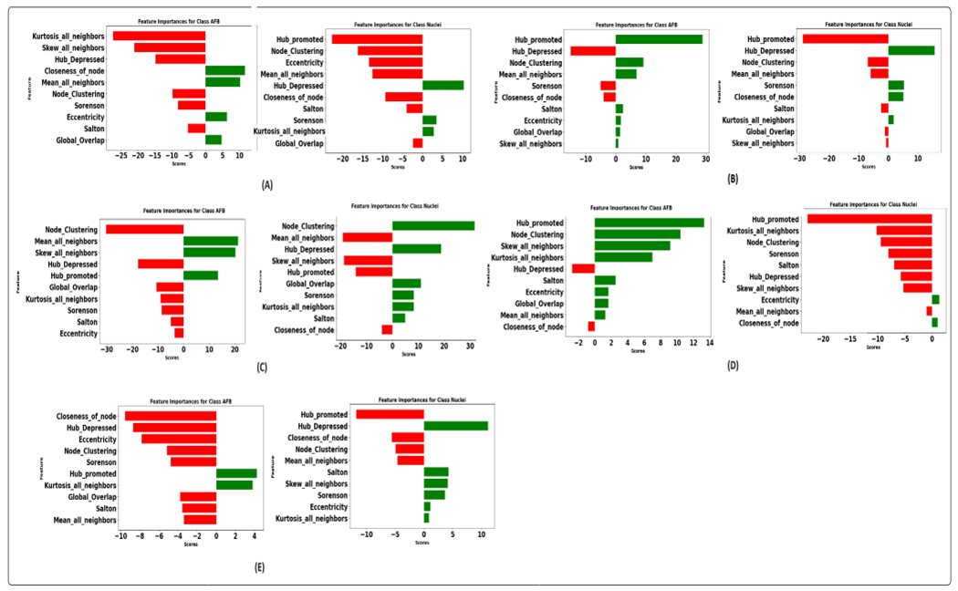
The construction of the graph is task-specific and significantly depends on domain knowledge. Therefore, a thorough evaluation is necessary to identify how much the geometric data affects the prediction tasks [37]. A comprehensive analysis was conducted using established model interpretation techniques to understand the influence of geometric (spatial) data and other features on the predictions. The SHAP method was employed for the machine learning models, whereas the integrated gradient technique was utilized for the graph-based models. These interpretative tools facilitate the identification of features that drive the predictive outcomes of the models. Additionally, the outcomes of these analyses were subjected to discussion and validation by domain experts to ensure the results' robustness and validity. The results of the SHAP summary plots to interpret the extent of each feature’s influence over the predictions are shown in the figure 13 and 14. These plots allowed us to identify which specific features substantially impact our model’s predictions. This section will focus on the models that demonstrated the best performance, namely XGBoost and CG-JKNN. As shown in figure 13, AFBs have a higher hub-promoted index than nuclei in the network; it indicates that the node representing AFB is connected to other nodes with a higher degree or number of connections.
FIGURE 13.
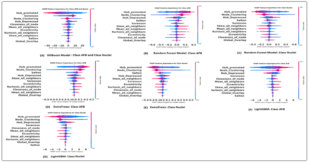
SHAP summary plot utilizing graph features: (A). XGBoost model. (B) and (C). Random forest model. (D) and (E). Extra trees model. (F) and (G). LightGBM model.
FIGURE 14.
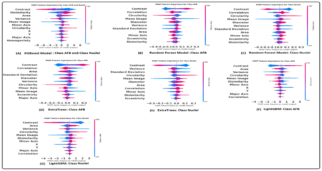
SHAP summary plot utilizing morphology features: (A). XGBoost model. (B) and (C). Random forest model. (D) and (E). Extra trees model. (F) and (G). LightGBM model.
The domain expert concurred with this observation as the bacteria’s ability to move around is contingent upon the host cell’s interaction with them. AFBs also have higher values for the closeness of nodes. This means that a node representing AFB plays a significant role in connecting different network parts and acts as a hub. This higher hub-promoted index suggests that the node denoting AFB strongly influences the overall network structure and information flow. According to the domain expert, it resonates with the biological context as the host’s inflammatory responses and immune system are triggered by the presence of the bacteria. We also see a higher node clustering coefficient for the node denoting AFB. It implies that the neighboring nodes of the node representing AFB are more likely to be connected, forming local clusters or communities. This can indicate a higher level of interconnectivity and cohesive structure around this node. They also have lower eccentricity values, suggesting that AFBs are more localized or closely connected within their immediate neighborhood or cluster of cells. This might align well with reality as the clusters of bacteria tend to replicate themselves. Their interactions with the host cell or granuloma environment are also local.
As shown in the figure 14, higher values of the contrast and lower values of circularity and area correspond to AFB. According to the expert, AFB exhibits distinct transitions or boundaries between different texture regions. This might be related to the unique cell wall properties of AFBs, which create sharp intensity transitions within the cells and give them well-defined edges or structures. The staining procedure involves using a red dye for AFB and a blue color for the other tissue. This might be the cause for higher GLCM contrast for the AFB. They are also smaller than the nucleus of activated macrophages and possess a rod shape compared to the disk-shaped nucleus. Pathologists also recognize AFB and macrophage nucleus with the help of circularity and size. AFBs tend to have higher values of variance. Bacterial cells have outer walls that surround them. These walls are made up of various molecules and structures. When we use a staining process to color the bacteria in an image, these walls can react differently to the staining. Some bacteria might have walls that absorb colors more efficiently, while others might absorb less colors. Bacteria with varying levels of absorbed red color will show higher variations in pixel intensities. This is because some parts of the bacteria will be intensely colored due to more absorbed color, while others will have lower pixel values due to less absorbed color.
Pathologists also rely on the chromatic pattern of the nucleus as a diagnostic indicator. GLCM features can potentially assess alterations in the pattern of nuclear chromatin [89], [90], [91]. The nucleus of the activated macrophage exhibited a lower energy value in its GLCM analysis. This lower energy value indicates that the texture patterns within this nucleus are characterized by non-uniformity, suggesting variations and irregularities in its structure. As per the insights from domain experts, the nucleus showcases a range of chromatin patterns with dense and sparse configurations. Figure 12 shows an example of both the patterns. Lower energy values can be attributed to the nature of the chromatin pattern. However, it is worth noting that domain experts consider the nuclear chromatin pattern as a final step for distinguishing between macrophage nucleus and AFB. Their initial approach involves assessing circularity, size, and color as primary factors for differentiation.
FIGURE 12.
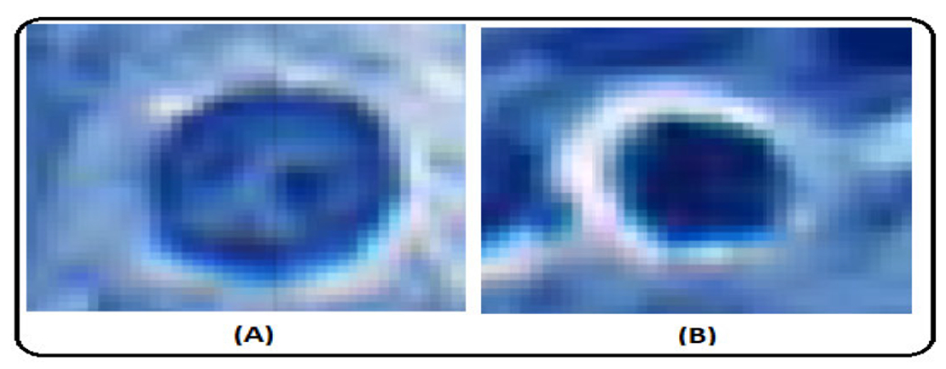
Nucleus of activated macrophage. (A). Sparse chromatin pattern. (B). Dense chromatin pattern.
Figure 15 illustrates the integrated gradient feature attribution results of morphology features using different graph models. The results of our proposed graph model exhibit a high degree of agreement with both the XGBoost model and the domain expert’s insights. Specifically, for class AFB, the feature attribution analysis reveals that the model assigns negative scores to perimeter and homogeneity while assigning a positive score to variance. These findings closely align with the domain expert’s qualitative analysis, confirming the model’s interpretability. Additionally, there is a strong inverse correlation between homogeneity and contrast [92]. This implies that instances belonging to class AFB tend to exhibit higher contrast. This observation aligns with the practices of domain experts who frequently rely on assessing contrast as a critical feature during their analytical processes. Similarly, for the instances within the class macrophage nucleus, our feature attribution analysis shows that a negative score is allocated to eccentricity, indicating that nuclei tend to have lower eccentricity values, implying a more circular or less elongated shape. The nucleus also has a higher homogeneity score than AFB, suggesting lower contrast. Furthermore, the negative score assigned to the variance indicates that the nucleus consistently and uniformly absorbs the stain. Figure 16 illustrates graph features’ integrated gradient feature attribution results using different graph models. CG-JKNN agrees with XGBoost for the AFB class, demonstrating a higher score for features such as the mean of all neighbors and node closeness and a lower score for the hub-depressed index. In contrast, for detecting nucleus, CG-JKNN assigns a lower score for the hub-promoted index, node closeness, and node clustering but a higher score for the hub-depressed index. The model interpretation results highlight how closely the models align with the insights of domain experts.
FIGURE 15.
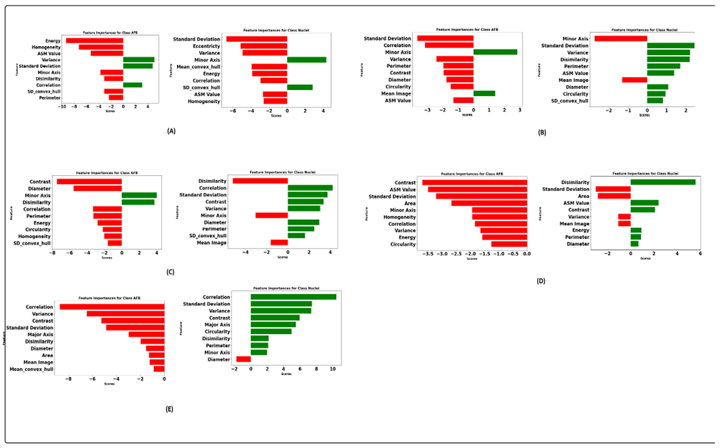
Integrated gradient feature attribution utilizing morphology features: (A). Proposed model. (B). GraphSAGE with max aggregator (C). GraphSAGE with mean aggregator (D). GATConv. (E). GATV2.
FIGURE 16.
Integrated gradient feature attribution utilizing graph features: (A). Proposed model. (B). GraphSAGE with max aggregator (C). GraphSAGE with mean aggregator (D). GATConv. (E). GATV2.
VII. RESULTS OF XGBOOST MODEL (TOP PERFORMING MODEL) WITH TOP K GRAPH AND MORPHOLOGY FEATURES
We trained the XGBoost model by gradually adding features based on their importance from a SHAP plot (Features are sorted in descending order by Shapley values). We started with the most important feature, then added the next one, and so on, until we included the top 11 features. When we added a new feature for each step, we trained the model again. At every step, we checked how well the model did by looking at the accuracy, F1 score, and AUPRC on the test set. This experiment was conducted with morphology and graph-based features.
The table 10 presents the performance of the XGBoost model as it sequentially incorporates the top K morphology features identified from a SHAP analysis. As more features are added (increasing K value), there is a general trend of improvement across all three metrics. This suggests that each additional feature provides new information that helps the model make better predictions. The F1 score also shows an upward trend. It starts at 0.65 for K=1 and goes up to 0.82 for K=11. The AUPRC value starts at 0.71 and increases to 0.8565. Figure 17 shows the performance plot with morphology features.
TABLE 10.
Performance metrics achieved with morphology features for every K value.
| K Value | Test Accuracy | Test F1 score | Test AUPRC |
|---|---|---|---|
| 1 | 0.727148237 | 0.651203501 | 0.713969089 |
| 2 | 0.763916467 | 0.69669247 | 0.751091436 |
| 3 | 0.786922287 | 0.719184263 | 0.772249125 |
| 4 | 0.796439575 | 0.727022312 | 0.78117288 |
| 5 | 0.821225608 | 0.763260495 | 0.808666456 |
| 6 | 0.82978432 | 0.773464553 | 0.81772094 |
| 7 | 0.842177337 | 0.787420456 | 0.83110704 |
| 8 | 0.850393701 | 0.799375631 | 0.840057218 |
| 9 | 0.86203355 | 0.816065723 | 0.852615778 |
| 10 | 0.865183156 | 0.819870094 | 0.856086222 |
| 11 | 0.865525505 | 0.820113574 | 0.856493032 |
FIGURE 17.

Morphology features (A). Plot of accuracy versus K. (B). Plot of F1 Score versus K. (C). Plot of AUPRC versus K.
The table 11 presents the performance of the XGBoost model as it sequentially incorporates the top K graph features identified from a SHAP analysis. As more features are added (increasing K value), there is an improvement across all three metrics (similar to morphology features). Figure 18 shows the performance plot with graph features.
TABLE 11.
Performance metrics achieved with graph features for every K value.
| K Value | Test Accuracy | Test F1 score | Test AUPRC |
|---|---|---|---|
| 1 | 0.726350088 | 0.623723834 | 0.731050091 |
| 2 | 0.87351103 | 0.852534562 | 0.878307163 |
| 3 | 0.916190374 | 0.898872059 | 0.920405592 |
| 4 | 0.914908392 | 0.897378084 | 0.919122938 |
| 5 | 0.925965493 | 0.911039795 | 0.92925645 |
| 6 | 0.933710806 | 0.91976466 | 0.937584011 |
| 7 | 0.941028791 | 0.92863607 | 0.944584073 |
| 8 | 0.945836227 | 0.934453782 | 0.949200114 |
| 9 | 0.9490946 | 0.93848835 | 0.952099228 |
| 10 | 0.9490946 | 0.938512162 | 0.952039998 |
| 11 | 0.949521927 | 0.939020456 | 0.952469116 |
FIGURE 18.

Graph features (A). Plot of accuracy versus K. (B). Plot of F1 Score versus K. (C). Plot of AUPRC versus K.
While the XGBoost model trained with the top 11 SHAP-selected features shows promising results, it is essential to note that there is a slight decrease in performance when compared to the model trained with all features. Specifically, the model with all features (as seen from the table 7) achieves a test accuracy of 86.8%, a test F1 score of 0.829, and a test AUPRC of 0.8654. In contrast, the model with the top 11 features achieves a test accuracy of 86.5%, an F1 score of 0.82, and an AUPRC of 0.856. However, the reduced model with 11 features still performs quite close to the full model, which speaks to the effectiveness of SHAP-based feature selection.
Next, when we utilized the full suite of graph features, it resulted in a test accuracy of 97.77%, an F1 score of 0.9734, and an AUPRC of 0.9797, as seen in Table 6. Upon applying feature selection to our XGBoost model and choosing the top 11 features indicated by the SHAP plot, there was a slight decrease in performance compared to using all features. The test accuracy decreased from 97.77% to 94.95%, the F1 score from 0.9734 to 0.9390, and the AUPRC from 0.9797 to 0.9525.
The table detailing the mean and standard deviation of the top K morphology features, as identified by the SHAP analysis, for both AFB and macrophage nucleus samples are shown in table 14. For the ‘Contrast’ feature, our data table indicates that the AFB has a higher mean value (on average, samples classified as AFB tend to have a greater ‘Contrast’ value) than the macrophage nucleus. Looking at the SHAP plot, we find that higher ‘Contrast’ values (indicated by the red color) are more associated with the AFB. Feature ‘Dissimilarity’ has a higher mean value for the macrophage nucleus, which is consistent with the SHAP plot’s indication that higher values of ‘Dissimilarity’ are influential in predicting the macrophage nucleus. Upon analyzing the ‘Homogeneity’ feature, we observe a relatively small difference in mean values between the AFB and macrophage nucleus. This is also reflected in the SHAP analysis, where ‘Homogeneity’ demonstrates lower importance than other features. The more minor mean difference suggests that ‘Homogeneity’ is not critical in distinguishing between the two classes.
TABLE 14.
Mean and standard deviation of top K morphology features.
| Feature | Class | Mean | Standard Deviation | Feature | Class | Mean | Standard Deviation |
|---|---|---|---|---|---|---|---|
| Contrast | AFB | 646.2373865 | 396.8268519 | Contrast | Nuclei | 277.2003633 | 148.4284912 |
| Dissimilarity | AFB | 11.01069996 | 3.603985191 | Dissimilarity | Nuclei | 14.20189472 | 2.595008892 |
| Area | AFB | 601.075684 | 349.4440592 | Area | Nuclei | 799.9927811 | 324.6724006 |
| Variance | AFB | 1729.357846 | 702.181662 | Variance | Nuclei | 1341.688406 | 673.6550925 |
| Mean Image | AFB | 114.9900388 | 20.90206066 | Mean Image | Nuclei | 115.9660491 | 24.40160937 |
| Minor Axis | AFB | 26.13620804 | 9.390976421 | Minor Axis | Nuclei | 30.19215891 | 8.608271603 |
| Circularity | AFB | 0.286050579 | 0.145519674 | Circularity | Nuclei | 0.382546318 | 0.19272632 |
| X | AFB | 22928.19947 | 12815.17536 | X | Nuclei | 23783.46309 | 11294.84367 |
| Y | AFB | 21116.11055 | 10360.14116 | Y | Nuclei | 19488.45966 | 11328.62783 |
| Major Axis | AFB | 40.54857861 | 9.474486534 | Major Axis | Nuclei | 41.74726661 | 8.220087311 |
| Homogeneity | AFB | 0.131664255 | 0.026637661 | Homogeneity | Nuclei | 0.144224389 | 0.026481044 |
The table detailing the mean and standard deviation of the top K graph features identified by the SHAP analysis for both AFB and macrophage nucleus samples is shown in Table 12. For the ‘Hub Promoted’ feature, our data table indicates that the AFB has a higher mean value than the macrophage nucleus. When we look at the SHAP plot, we find that higher ‘Hub Promoted’ values (indicated in red) are more associated with the class AFB. For the AFB, the ‘Sorenson’ feature has a mean of approximately 59.55 and a standard deviation of about 61.24. For the macrophage nucleus, the mean is significantly higher at 95.15, with a standard deviation of approximately 71.56, which is consistent with the SHAP plot’s indication that higher values of ‘Sorenson’ are influential in predicting the macrophage nucleus. The ‘Global_Overlap’ feature, as observed in our dataset, exhibits minimal differences in its mean values between the AFB and macrophage nucleus. The feature ‘Global_Overlap’, as seen from our statistics table, does not vary significantly between the two classes. Corroborating this, the SHAP feature importance plot places ‘Global_Overlap’ at the lower end of the spectrum, indicating its relatively minor role in influencing the model’s predictions compared to other features.
TABLE 12.
Mean and standard deviation of top K graph features.
| Feature | Class | Mean | Standard Deviation | Feature | Class | Mean | Standard Deviation |
|---|---|---|---|---|---|---|---|
| Hub_promoted | AFB | 136.4581739 | 84.26090681 | Hub_promoted | Nuclei | 68.0801658 | 68.03701789 |
| Sorenson | AFB | 59.54648759 | 61.23655717 | Sorenson | Nuclei | 95.15423665 | 71.56260057 |
| Node_Clustering | AFB | 0.783554612 | 0.073479537 | Node_Clustering | Nuclei | 0.61096627 | 0.175413699 |
| Hub_Depressed | AFB | 54.05654923 | 56.46057638 | Hub_Depressed | Nuclei | 79.4676893 | 64.29050645 |
| Closeness_of_node | AFB | 4.542566512 | 4.071530728 | Closeness_of_node | Nuclei | 4.150767665 | 3.636215078 |
| Mean_all_neighbors | AFB | 22.53811236 | 122.2853582 | Mean_all_neighbors | Nuclei | 10.07845304 | 45.3923509 |
| Eccentricity | AFB | 16.18867582 | 4.85997634 | Eccentricity | Nuclei | 15.28154962 | 4.325327836 |
| Kurtosis_all_neighbors | AFB | −0.014420408 | 1.296525604 | Kurtosis_all_neighbors | Nuclei | −0.447366478 | 0.905347493 |
| Skew_all_neighbors | AFB | 0.400163852 | 0.548024782 | Skew_all_neighbors | Nuclei | 0.073265344 | 0.502343919 |
| Salton | AFB | 100.9123406 | 72.42727025 | Salton | Nuclei | 60.27787393 | 61.67832625 |
| Global_Overlap | AFB | 2.48E-05 | 0.013335022 | Global_Overlap | Nuclei | 0.00054195 | 0.02069925 |
Also, it is essential to differentiate between the variability of a feature’s influence on model predictions, as illustrated by the spread of SHAP values, and the dispersion of the feature’s actual values within the dataset, quantified by the standard deviation. The spread in SHAP values depicted in the SHAP feature importance plot reflects the range of influence that the feature exerts across different instances in the model’s predictions. This influence variability is separate from the standard deviation of the feature’s values. The standard deviation is a separate statistical measure that indicates the extent to which the feature values are spread around their mean in the dataset.
VIII. ABLATION STUDIES
Four pivotal ablation studies were undertaken to assess the robustness of our models. The first study focused on establishing consensus across models trained on distinct subsets of train-validation and test data. This investigation aimed to reveal the models’ generalization capabilities and ability to deliver consistent results regardless of dataset variations. The second study investigated the impact of morphology and graph-based features on model performance. By integrating these distinct feature sets, we aimed to determine their effects on improving the predictive capabilities. The third study dealt with measuring the performance with different node aggregation mechanisms. The fourth and final ablation study evaluated the effectiveness of the jumping knowledge technique implemented in our model. This study involved conducting experiments both with and without the application of jumping knowledge.
A. MODEL CONSENSUS: EFFECT OF RANDOM WEIGHTS INITIALIZATION AND DIFFERENT SUBSETS OF DATA
We conducted experiments to explore whether the consensus (in terms of feature stability) [93] among models varies across different subsets of training, validation, and test data. We generated SHAP summary plots for each ML model using these distinct subsets and extracted the top 6 features from each plot. Similarly, we followed a similar procedure for the graph models but selected the top 6 features from the integrated gradient plots. This process allowed us to derive the final consensus among the models. Figure 19 shows the consensus among the ML models concerning both graph and morphology features.
FIGURE 19.
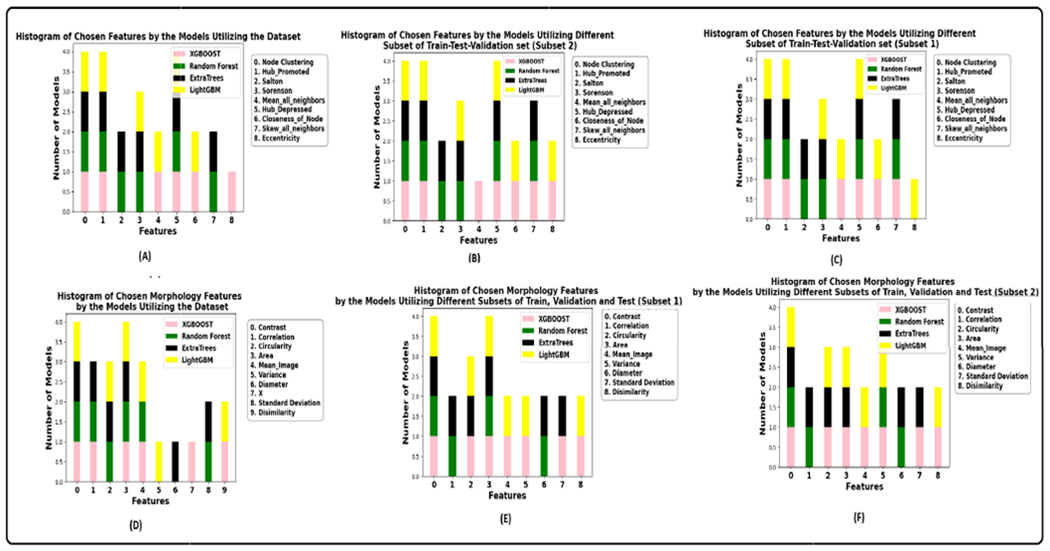
ML model consensus for class AFB and class macrophage nucleus; Upper Row: Graph Features (A). Consensus among the models while using the best-performing split. (B). Consensus among the models while using a different subset of the train-val-test set. (C). Consensus among the models while using another subset of the train-val-test set. Lower Row: Morphology Features (D). Consensus among the models while using the best-performing split. (E). Consensus among the models while using a different subset of the train-val-test set. (F). Consensus among the models while using another subset of the train-val-test set.
During our experiments, we noticed that SHAP summary plots (not shown here) consistently highlighted the same features, with minor variations in their ranking order. Several factors contribute to the consistent feature importance rankings observed in our analysis. Firstly, the selected features may exhibit a high degree of robustness and informativeness across various subsets of the data. These features consistently capture essential patterns and relationships, even when trained on different data samples. Additionally, the inherent regularization mechanisms employed by the machine learning models used in our analysis play a pivotal role. The regularization techniques, such as feature sampling and depth limitations, contribute to the stability of feature importance rankings [94]. We also conducted experiments using graph-based models with random weight initialization to investigate the variability in feature attribution. Specifically, we were interested in observing whether the selection of influential features changed across different trials of the model. In our study, we conducted three separate trials for the proposed model.
Figure 20 and 21 illustrate the feature attribution results for class AFB and class macrophage nucleus averaged across the test instances for the three trials. The term ‘nuclei’ refers to the macrophage nucleus. We observed variations in the morphology features identified as influential in each trial, although some similarities were also observed. This is due to random weight initialization that leads to different starting points for the model’s parameters in each run. These initial differences can set the model on distinct learning trajectories, causing it to assign varying importance to features during training. We observed a relatively slight variation in the choice of graph features, as the model consistently selected almost the same set of features (with differences in importance scores) in each trial, as seen in Figure 21. The consistent selection of these specific graph features across multiple trials with random weight initialization shows their robustness and impact on the model’s predictions. Figure 22 shows the consensus among the graph models that yielded the best results across the three trials, considering each of the feature sets.
FIGURE 20.
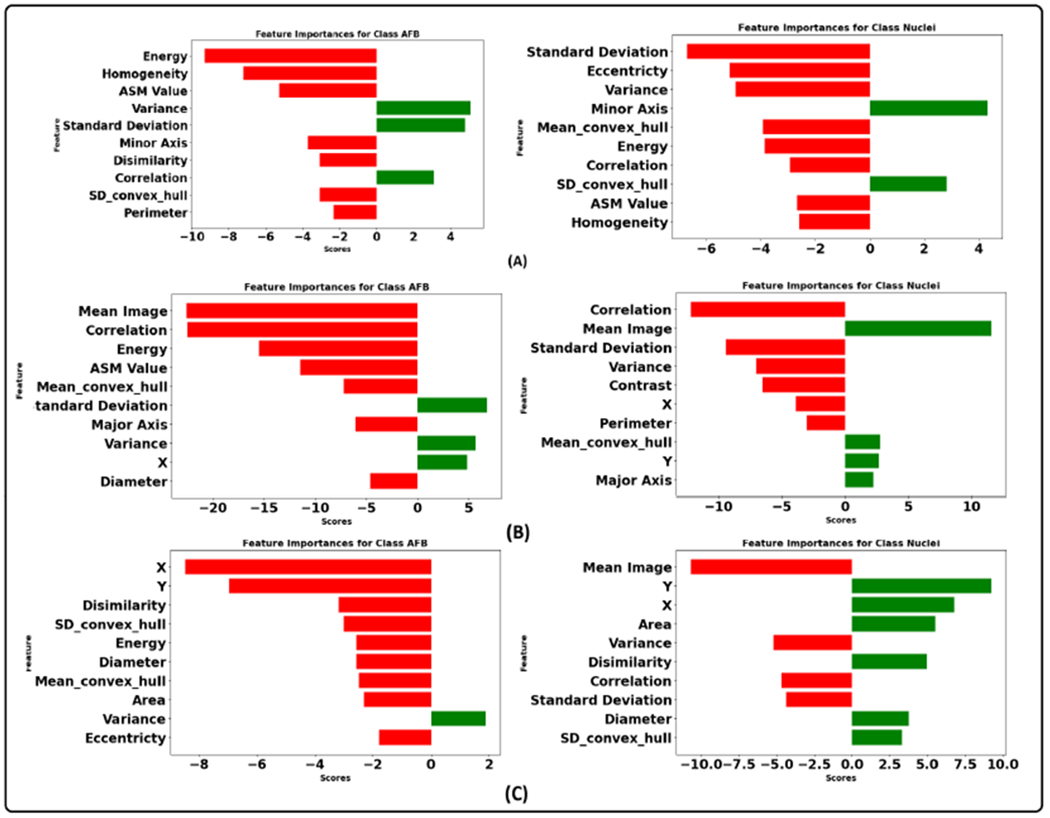
Integrated gradient feature attribution by employing proposed model utilizing the morphology features (A). Attribution scores of features for class AFB and class macrophage nucleus during the run 1. (B). Attribution scores of features for class AFB and class macrophage nucleus during the run 2. (C). Attribution scores of features for class AFB and class macrophage nucleus during the run 3.
FIGURE 21.
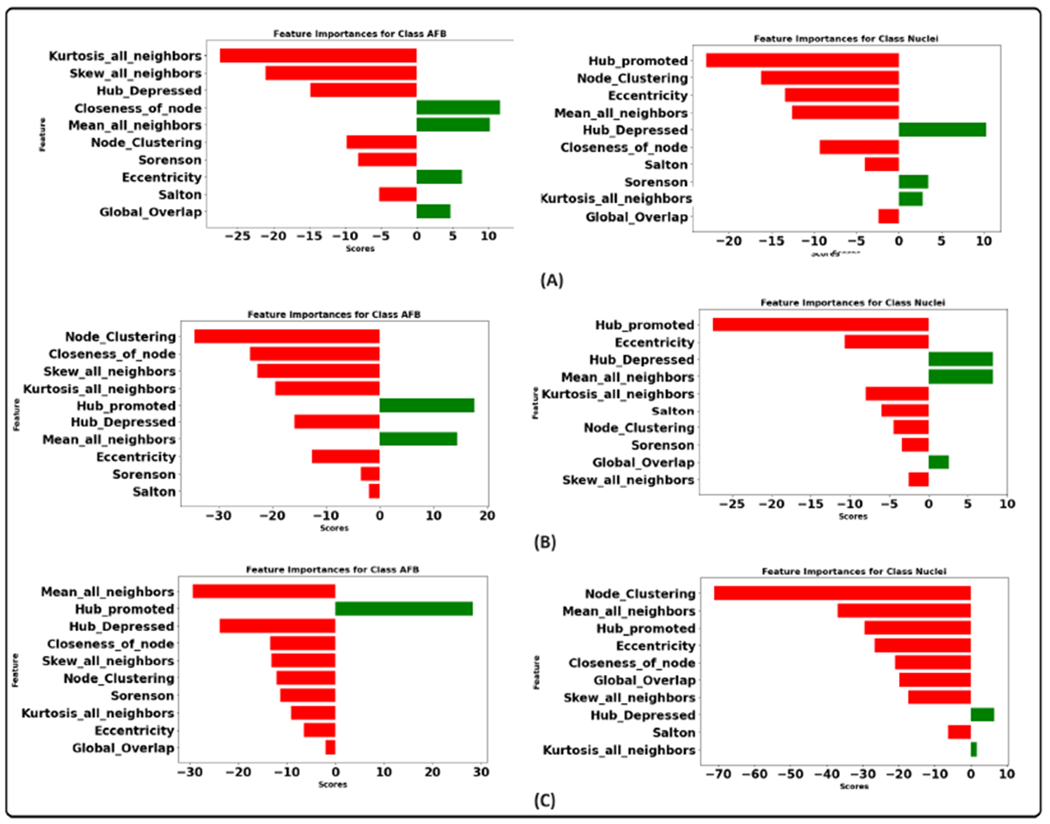
Integrated gradient feature attribution by employing proposed model utilizing the graph features (A). Attribution scores of features for class AFB and class macrophage nucleus during the run 1. (B). Attribution scores of features for class AFB and class macrophage nucleus during the run 2. (C). Attribution scores of features for class AFB and class macrophage nucleus during the run 3.
FIGURE 22.
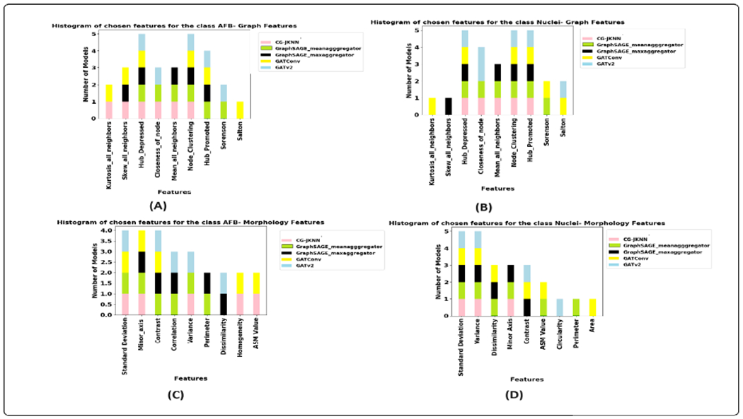
Graph model consensus for class AFB and class macrophage nucleus; Upper row: Graph features (A). Consensus among the models for class AFB. (B). Consensus among the models for class macrophage nucleus. Lower Row: Morphology Features (C). Consensus among the models for class AFB. (D).Consensus among the models for class macrophage nucleus.
By comparing Figure 19 and Figure 22, it is evident that both the ML models and graph models consistently highlight the importance of hub-promoted index, hub-depressed index, and node clustering as top features for the classification. Regarding morphological features, models consistently opt for contrast and variance as the top features. Notably, while global graph features may not be extremely useful in node-level classification, their relevance will be seen for graph-level classification, mainly when categorizing M.tb infected DO mice samples into Supersusceptible Progressor, Asymptomatic Controller and Susceptible Controller categories [95].
B. EFFECT OF NODE FEATURES
We constructed the cell graph using morphological and graph features to test their effectiveness. We also trained the ML models with these feature sets. We will refer to this specific combination of features throughout the rest of the article as the “combined feature set”. The results can be seen in Table 15 and 16. The test F1 score of XGBoost using morphological features is 15.23% lower than the model with combined features, highlighting the importance of cell structure for node classification. The test f1 score with graph features is 0.79% below the score with combined features, demonstrating the significance of the structural relationships and interactions between cells within the tissue sample. The combination of morphological and graph-based features provides the best predictive power for our model. The AUPRC results for both ML and graph-based models using combined features on the test set are presented in Figure 23. While morphological features are informative, they do not perform well independently. Likewise, graph-based features are helpful but benefit from integrating morphological features to achieve the highest F1 score on the test data. We see similar results in graph-based models. When utilizing combined features, the CG-JKNN model achieved a test F1 score, surpassing its performance with only graph features by 4.35% and exceeding its results with just morphological features by 9.39%.
TABLE 15.
Combined features: performance and hyperparameters of ML models.
| Model | Train_Acc | Val_Acc | Test_Acc | Train_F1 | Val_F1 | Test_F1 | Hyperparameters |
|---|---|---|---|---|---|---|---|
| XGBoost | 99.99 | 98.7 | 98.56 | 0.99 | 0.9832 | 0.9813 | gamma=0.073,learning_rate=0.2459, max_depth=10, estimators=171, reg_alpha=0.2, reg_lambda=0.3 |
| Random Forest | 99.83 | 96.76 | 96.41 | 0.9979 | 0.9579 | 0.95328 | min_samples_leaf=1, min_samples_split=9, estimators=112,max_depth=30 |
| LightGBM | 99.76 | 98.25 | 98.21 | 0.9969 | 0.9774 | 0.9768 | lr=0.313, max_depth= 23, min_child_samples=12, num_leaves=46,max_depth= 23 |
| Extra Trees | 99.35 | 96.33 | 95.8 | 0.9916 | 0.9528 | 0.9461 | min_samples_leaf=1, min_samples_split=3, estimators=100, max_depth=20 |
TABLE 16.
Combined features: performance and hyperparameters of graph models.
| Model | Train_Acc | Val_Acc | Test_Acc | Train_F1 | Val_F1 | Test_F1 | Hyperparameters |
|---|---|---|---|---|---|---|---|
| GraphSAGE_mean | 95.136 ±0.07 | 90.183 ±0.069 | 86.656 ±0.209 | 0.9605 ±0.001 | 0.9532 ±0.003 | 0.8972 ±0.004 | hidden dim=78, lr=0.0054, dropout=0.1975, Aggr=mean |
| GraphSAGE_max | 93.04 ±0.65 | 88.57 ±0.655 | 84.593±0.499 | 0.9261 ±0.015 | 0.9111 ±0.025 | 0.9092±0.012 | hidden dim=78, lr=0.0054, dropout=0.1975, Aggr=max |
| GATV2 | 93.30 ±0.28 | 89.68 ±0.88 | 83.78±1.013 | 0.9448 ±0.024 | 0.9359 ±0.014 | 0.8975±0.025 | lr=0.012,heads=8, dropout=0.1, weight_decay=5e-4 |
| GatConv | 90.38 ±1.28 | 87.38 ±1.34 | 81.73±1.136 | 0.9524±0.012 | 0.948 ±0.013 | 0.8818±0.031 | lr=0.073,heads=8, dropout=0.111, weight_decay=0.0005 |
| Proposed Model | 94.50 ±0.385 | 89.86 ±0.194 | 87.23 ±0.172 | 0.9642 ±0.001 | 0.9601 ±0.007 | 0.9509 ±0.004 | lr=0.001, dropout=0.1 num_sage_layers=3, hidden_channel=33 |
FIGURE 23.
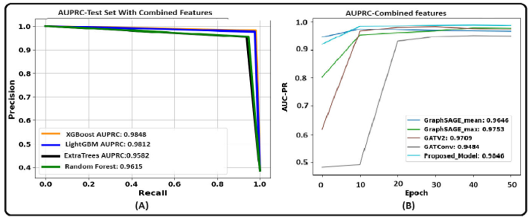
Area under the precision-recall curve of ML models and graph based models with combined feature set (A). Performance of ML models (B). Performance of graph based models.
However, despite these improvements, the XGBoost model still outperforms the CG-JKNN. The upper bound of trainable parameters in the XGBoost model is estimated based on the maximum potential size of each decision tree. For a tree of maximum depth ‘d’, the total number of nodes (and hence parameters) is approximately 2Λ(d + 1) − 1. When multiplied by the number of trees (‘n_estimators’), this gives us an overall upper bound. According to our calculations, assuming each tree grows to its maximum depth, which might not always be the case due to pruning, the total number of parameters is approximately 171 · (2Λ11) − 1, equaling 350,037. Table 15 indicates that the gamma value is too small to result in significant pruning.
Despite the current performance gap, we believe that the efficiency of GNN models like CG-JKNN can be substantially improved through the concept of knowledge distillation [96]. This technique could enable these models to achieve performance comparable to XGBoost while requiring significantly fewer parameters. This approach allows us to simultaneously make GNN models better and more efficient, meeting the need for models that work well without requiring significant computing power.
C. IMPACT OF DIFFERENT NODE AGGREGATION TECHNIQUE
One of the pivotal operations within graph neural networks is the aggregation process. Its primary objective is to systematically exploit the information from neighboring nodes, leading to the gradual updation of the target node’s latent representation [97]. We investigate the impact of two aggregation techniques: Mean aggregator and Max aggregator [25], [98]. The experimental results can be seen in Table 17. The plot of the AUPRC on the test set is shown in the figure 24. We achieved an F1-score of 0.8707 with mean aggregator and morphology features. Furthermore, we attained an even higher F1-score of 0.9157 using the mean aggregator with graph features. We chose the mean aggregator as our aggregation technique based on these results because it performs better than the max aggregator. Previous literature has consistently demonstrated the superiority of the mean aggregator over other aggregation techniques in node classification tasks [97], [98]. This is seen in the studies involving rich node features and where the distribution of the features in the neighborhood provides a strong and valuable signal, significantly enhancing the performance [98].
TABLE 17.
Ablation study on various aggregation techniques.
| Features | Aggregator | Train Acc | Val Acc | Test Acc | Train F1 | Val F1 | Test F1 |
|---|---|---|---|---|---|---|---|
|
| |||||||
| Morphology | Mean | 83.50 ±2.04 | 79.12 ±2.70 | 73.39 ±2.7 | 0.8132 ±0.005 | 0.7959 ±0.009 | 0.8617 ±0.009 |
| Max | 80.99 ±2.63 | 78.16 ±1.988 | 71.84 ±1.386 | 0.7409 ±0.038 | 0.749 ±0.058 | 0.787 ±0.049 | |
|
| |||||||
| Graph | Mean | 92.88 ±0.021 | 88.47 ±0.6276 | 87.21 ±0.984 | 0.9681 ±0.004 | 0.9603 ±0.005 | 0.9057 ±0.01 |
| Max | 89.143 ±0.122 | 86.92 ±0.412 | 84.84 ±0.239 | 0.8832 ±0.016 | 0.899 ±0.027 | 0.867 ±0.004 | |
|
| |||||||
| Combined | Mean | 94.503 ±0.385 | 89.863 ±0.194 | 87.233 ±0.172 | 0.9642 ±0.001 | 0.9601 ±0.007 | 0.9509 ±0.004 |
| Max | 92.97 ±0.6648 | 89.283 ±0.9871 | 80.53 ±2.09 | 0.9431 ±0.0007 | 0.957 ±0.011 | 0.9309 ±0.023 | |
FIGURE 24.

Performance of different aggregation techniques: (A). Proposed model with Mean and Max Aggregator and Graph Features. (B). Proposed model with Mean and Max Aggregator and Morphology Features. (C). Proposed model with mean and max aggregator and combined features.
D. IMPACT OF JUMPING KNOWLEDGE ON CG-JKNN
In this section, we learn the specific impact of the jumping knowledge technique on CG-JKNN’s performance. Previous works employing cell graph methodologies have demonstrated the efficacy of Jumping Knowledge, particularly in graph-level classification tasks [40], [41], [50]. To comprehensively assess this aspect, we conducted a series of experiments both with and without the implementation of jumping knowledge. Concatenation was selected among three jumping knowledge techniques: concatenation, max-pooling, and an LSTM-attention mechanism. The concatenation-based jumping knowledge technique aggregated node features across different layers rather than just the last layer. Our experiments were conducted with different feature sets, including graph features, morphology features, and a combination of both. To ensure the validity and reliability of our findings, we maintained consistency in the data points used across all experiments. This approach ensured that any observed changes in the model’s performance could be attributed directly to the presence or absence of jumping knowledge, thereby eliminating the potential influence of varying data points.
The results of the models are averaged over three trials. The table 18 presents a detailed comparison of the CG-JKNN model’s performance using graph-based features, both with and without the incorporation of jump knowledge. Table 19 presents a detailed comparison of the CG-JKNN model’s performance using morphology-based features, both with and without the incorporation of jump knowledge, and table 20 presents a detailed comparison of the CG-JKNN model’s performance using combined features, both with and without the incorporation of jump knowledge.
TABLE 18.
Graph features: comparison of proposed model with and without jump knowledge.
| Model | Train_Acc | Val_Acc | Test_Acc | Train_F1 | Val_F1 | Test_F1 |
|---|---|---|---|---|---|---|
| Proposed Model with Jump Knowledge | 92.88 ± 0.021 | 88.47 ± 0.62 | 87.21 ± 0.98 | 0.9681 ± 0.004 | 0.9603 ± 0.005 | 0.9057 ± 0.01 |
| Proposed Model without Jump Knowledge | 89.57 ± 1.029 | 87.67 ± 1.889 | 85.30 ± 0.755 | 0.883 ± 0.005 | 0.8981 ± 0.0171 | 0.892 ± 0.0018 |
TABLE 19.
Morphology features: comparison of proposed model with and without jump knowledge.
| Model | Train_Acc | Val_Acc | Test_Acc | Train_F1 | Val_F1 | Test_F1 |
|---|---|---|---|---|---|---|
| Proposed Model with Jump Knowledge | 83.5 ± 2.047 | 79.12 ± 2.70 | 73.39 ± 1.23 | 0.813 ± 0.005 | 0.795 ± 0.009 | 0.861 ± 0.012 |
| Proposed Model without Jump Knowledge | 78.42 ± 0.473 | 78.06 ± 0.422 | 75.685 ± 1.657 | 0.765 ± 0.016 | 0.8139 ± 0.031 | 0.82 ± 0.006 |
TABLE 20.
Combined features: comparison of proposed model with and without jump knowledge.
| Model | Train_Acc | Val_Acc | Test_Acc | Train_F1 | Val_F1 | Test_F1 |
|---|---|---|---|---|---|---|
| Proposed Model with Jump Knowledge | 94.50 ± 0.385 | 89.86 ± 0.194 | 87.23 ± 0.172 | 0.9642 ± 0.001 | 0.9601 ± 0.007 | 0.9509 ± 0.004 |
| Proposed Model without Jump Knowledge | 91.72 ± 0.765 | 88.77 ± 0.9073 | 86.19 ± 1.06 | 0.9306 ± 0.033 | 0.927 ± 0.027 | 0.9057 ± 0.0109 |
When analyzing the performance of our models using graph features, as seen from the table 18, the F1 scores show improvement with jump knowledge across training, validation, and test datasets. The Train F1 score sees an increase from 0.883±0.005 to 0.9681±0.0040, the val F1 score improves from 0.8981±0.0171 to 0.9603±0.005, and the test F1 improves from 0.892±0.0018 to 0.9057±0.01. The utilization of jumping knowledge alongside morphological features exhibits a consistent trend of performance improvement, mirroring the improvements seen with graph features. Train F1 score rises from 0.765±0.016 to 0.813±0.005, and test F1 score increases from 0.82±0.006 to 0.861±0.012. When analyzing the performance of our models using combined features, the addition of jumping knowledge led to substantial improvements in the F1 scores across all evaluation phases. For the training phase, the F1 score increased from 0.9306 ±0.033 to 0.9642±0.001. During validation, we observed an improvement in the F1 score from 0.927 ±0.027 to 0.9601± 0.007. The test F1 score, indicative of the model’s performance on new data, also improved from 0.9057±0.0109 to 0.9509±0.004. AUPRC results (obtained after 50 epochs), as shown in Figure 25 across various feature sets, clearly demonstrate that incorporating jumping knowledge consistently improves performance.
FIGURE 25.
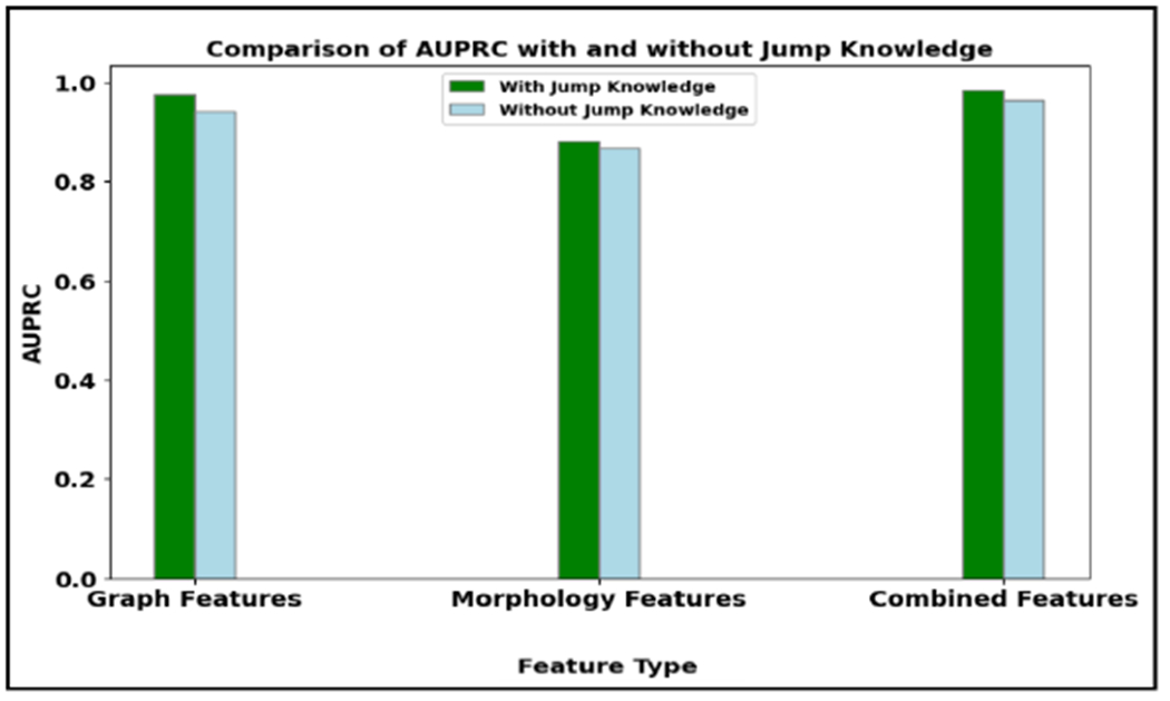
Comparison of AUPRC with and without jump knowledge with different feature sets.
IX. CONCLUSION AND FUTURE DIRECTIONS
In our study, we introduce the CG-JKNN model, a cell graph convolutional network integrating the ‘jumping knowledge’ mechanism, offering a new perspective in analyzing GNNs with cell graphs. Our unique approach in constructing cell graphs focuses on mycobacterium bacteria’s cords and the radius of the activated macrophage nucleus in activated macrophages, reflecting actual cellular interactions within the granuloma. The CG-JKNN model effectively combines morphological features with spatial information of cells, showing promising results compared to classical GNN architectures. Notably, XGBoost outperforms other ML models, indicating the effectiveness of cell graph-derived features. We have also integrated model interpretation techniques, revealing key features such as contrast, circularity, and area that align with domain expert insights. The model’s attention to attributes like node clustering mirrors cellular interconnections in the tissue microenvironment. However, our approach faces limitations due to the small dataset size and the need to consider temporal dynamics in disease progression. For future work, we aim to categorize M.tb-affected DO mice samples into three groups at the graph level: Supersusceptible Progressor, Asymptomatic Controller, and Susceptible Controller. We also plan to expand the dataset and develop a more complex teacher model for knowledge distillation, assessing the performance of our proposed model in comparison with Scalable Inception Graph Neural Networks.
TABLE 1.
Abbreviations and acronyms.
| TB | Tuberculosis |
| ZN | Ziel-Neelsen |
| AFB | Acid Fast Bacilli |
| CG | Cell Graph |
| JKNN | Jumping Knowledge Neural Network |
| WSI | Whole Slide Image |
| GNN | Graph Neural Network |
| XGBoost | Extreme Gradient Boosting |
| GAT | Graph Attention Network |
| DO | Diversity Outbred |
| ML | Machine Learning |
| SHAP | Shapely Additive Explanation |
| TME | Tissue Microenvironment |
| AUPRC | Area under the precision-recall curve |
| GLCM | Gray Level Co-Occurrence Matrix |
| IGRA | Interferon-gamma Releasing Assay |
| SVM | Support Vector Machine |
| KNN | K-Nearest Neighbors |
| MLP | Multilayer perception |
| GIN | Graph Isomorphism Network |
| AUC | Area under the ROC Curve |
TABLE 13.
Performance achieved with top 11 features.
| Feature | Model | Train_Acc | Val_Acc | Test_Acc | Train_F1 | Val_F1 | Test_F1 | Train_AUPRC | Val_AUPRC | Test_AUPRC |
|---|---|---|---|---|---|---|---|---|---|---|
| Morphology | XGBoost | 88.2179 | 86.54 | 86.552 | 0.84675 | 0.8229 | 0.82011 | 0.87841 | 0.86038 | 0.85649 |
| Graph | XGBoost | 95.489 | 94.9842 | 94.952 | 0.945 | 0.939 | 0.939 | 0.9578 | 0.9529 | 0.952 |
ACKNOWLEDGMENT
The assistance from the National Institutes of Health NHLBI and Boehringer Ingelheim Veterinary Scholars Program has been instrumental in advancing their research.
The work of Diana Choi was supported by the Boehringer Ingelheim Veterinary Scholars Program. The work of Gillian Beamer was supported by the National Institutes of Health National Heart, Lung, and Blood Institute (NHLBI) under Grant R01HL14541.
Biographies

VASUNDHARA ACHARYA received the B.E. degree in information science and engineering from the N.M.A.M. Institute of Technology, Nitte, the M.Tech. degree in software engineering from the Manipal Institute of Technology (M.I.T.), Manipal Academy of Higher Education (M.A.H.E.), Manipal, and the master’s degree in computer science from the Rensselaer Polytechnic Institute (RPI), where she is currently pursuing the Ph.D. degree with the Department of Computer Science. Her current interests include medical image processing and the application of artificial intelligence in healthcare.

DIANA CHOI received the degree in biology from the Mount Holyoke College, MA, USA, and the Doctor of Veterinary Medicine degree from the Cummings School of Veterinary Medicine, Tufts University, North Grafton, MA. She is a Veterinarian with the Symphony Vet Center, New York. Her interests include cardiology, dermatology, ultrasonography, and diagnostic imaging.

BÜLENT YENER (Fellow, IEEE) received the M.S. and Ph.D. degrees in computer science from Columbia University, in 1987 and 1994, respectively. He is a Professor with the Department of Computer Science with a courtesy appointment in the ECSE Department, Rensselaer Polytechnic Institute (RPI), Troy, NY, USA. He has been the Founding Director of the Data Science Research Center, and the Associated Director of IDEA, RPI. Before joining RPI, he was a member of the Technical Staff at Bell Laboratories, Murray Hill, NJ, USA. His current research interests include applied machine learning in bioinformatics, medical informatics, and cyber security. He is a Senior Member of ACM and a member of AAA.

GILLIAN BEAMER received the V.M.D. degree from the University of Pennsylvania, in 2000, and the Ph.D. degree from The Ohio State University, in 2009. She has completed a residency in veterinary anatomic pathology from The Ohio State University. She is a veterinary pathologist and a research scientist studying tuberculosis. She is an Adjunct Associate Professor and an Independent Staff Scientist with Texas Biomed. She has about 20 years of experience in veterinary medicine, pathology, and scientific research. She is a Board Certified Diplomate with the American College of Veterinary Pathologists. In 2022, she joined Texas Biomedical Research Institute, San Antonio, TX, USA, as an Adjunct Associate Professor; and Aiforia Inc., Cambridge, MA, USA, as the Director of research pathology.
Footnotes
This work involved human subjects or animals in its research. Approval of all ethical and experimental procedures and protocols was granted by the Tufts Institutional Animal Care and Use Committee (IACUC) (approved animal experiments) under Approval Nos. G2012-53, G2015-33, and G2018-33; and the Tufts Institutional Biosafety Committee (approved biohazardous infectious agent work) under Approval Nos. GRIA04, GRIA10, and GRIA17.
A. ABBREVIATIONS AND ACRONYMS
The abbreviations and acronyms used throughout the paper are tabulated in the Table 1.
ETHICS STATEMENT
Tufts Institutional Animal Care and Use Committee (IACUC) approved animal experiments under protocols G2012-53; G2015-33; G2018-33. Tufts Institutional Biosafety Committee approved biohazardous infectious agent work under registrations GRIA04; GRIA10; and GRIA17.
CONFLICTS OF INTEREST
The authors do not have any conflicts of interest to disclose.
REFERENCES
- [1].Bagcchi S, “Who’s global tuberculosis report 2022,” Lancet Microbe, vol. 4, no. 1, p. e20, 2023. [DOI] [PubMed] [Google Scholar]
- [2].Koyuncu D, Niazi MKK, Tavolara T, Abeijon C, Ginese M, Liao Y, Mark C, Gower AC, Gatti DM, Kramnik I, Gurcan M, Yener B, and Beamer G, “Tuberculosis biomarkers discovered using diversity outbred mice,” medRxiv, pp. 1–44, Jan. 2021. [DOI] [PMC free article] [PubMed] [Google Scholar]
- [3].Tavolara TE, Niazi MKK, Beamer G, and Gurcan MN, “Segmentation of mycobacteriumtuberculosis bacilli clusters from acid-fast stained lung biopsies: A deep learning approach,” Proc. SPIE, vol. 11320, pp. 92–98, Mar. 2020. [Google Scholar]
- [4].Lee J and Lee J, “A study of mycobacteriumtuberculosis detection using different neural networks in autopsy specimens,” Diagnostics, vol. 13, no. 13, p. 2230, Jun. 2023. [DOI] [PMC free article] [PubMed] [Google Scholar]
- [5].Soldevilla P, Vilaplana C, and Cardona P-J, “Mouse models for mycobacteriumtuberculosis pathogenesis: Show and do not tell,” Pathogens, vol. 12, no. 1, p. 49, Dec. 2022. [DOI] [PMC free article] [PubMed] [Google Scholar]
- [6].Yu K-H, Zhang C, Berry GJ, Altman RB, Ré C, Rubin DL, and Snyder M, “Predicting non-small cell lung cancer prognosis by fully automated microscopic pathology image features,” Nature Commun., vol. 7, no. 1, p. 12474, Aug. 2016. [DOI] [PMC free article] [PubMed] [Google Scholar]
- [7].Pati P, Jaume G, Foncubierta-Rodríguez A, Feroce F, Anniciello AM, Scognamiglio G, Brancati N, Fiche M, Dubruc E, Riccio D, Di Bonito M, De Pietro G, Botti G, Thiran J-P, Frucci M, Goksel O, and Gabrani M, “Hierarchical graph representations in digital pathology,” Med. Image Anal, vol. 75, Jan. 2022, Art. no. 102264. [DOI] [PubMed] [Google Scholar]
- [8].Hou L, Samaras D, Kurc TM, Gao Y, Davis JE, and Saltz JH, “Patch-based convolutional neural network for whole slide tissue image classification,” in Proc. IEEE Conf. Comput. Vis. Pattern Recognit. (CVPR), Jun. 2016, pp. 2424–2433. [DOI] [PMC free article] [PubMed] [Google Scholar]
- [9].Cruz-Roa A, Basavanhally A, González F, Gilmore H, Feldman M, Ganesan S, Shih N, Tomaszewski J, and Madabhushi A, “Automatic detection of invasive ductal carcinoma in whole slide images with convolutional neural networks,” Proc. SPIE, vol. 9041, Mar. 2014, Art. no. 904103. [Google Scholar]
- [10].Mousavi HS, Monga V, Rao G, and Rao AUK, “Automated discrimination of lower and higher grade gliomas based on histopathological image analysis,” J. Pathol. Informat, vol. 6, no. 1, p. 15, Jan. 2015. [DOI] [PMC free article] [PubMed] [Google Scholar]
- [11].Xu Y, Jia Z, Ai Y, Zhang F, Lai M, and Chang EI, “Deep convolutional activation features for large scale brain tumor histopathology image classification and segmentation,” in Proc. IEEE Int. Conf. Acoust., Speech Signal Process. (ICASSP), Apr. 2015, pp. 947–951. [Google Scholar]
- [12].Zhou Y, Chang H, Barner K, Spellman P, and Parvin B, “Classification of histology sections via multispectral convolutional sparse coding,” in Proc. IEEE Conf. Comput. Vis. Pattern Recognit, Jun. 2014, pp. 3081–3088. [DOI] [PMC free article] [PubMed] [Google Scholar]
- [13].Ciga O, Xu T, Nofech-Mozes S, Noy S, Lu F-I, and Martel AL, “Overcoming the limitations of patch-based learning to detect cancer in whole slide images,” Sci. Rep, vol. 11, no. 1, p. 8894, Apr. 2021. [DOI] [PMC free article] [PubMed] [Google Scholar]
- [14].van der Laak J, Ciompi F, and Litjens G, “No pixel-level annotations needed,” Nature Biomed. Eng, vol. 3, no. 11, pp. 855–856, Oct. 2019. [DOI] [PubMed] [Google Scholar]
- [15].Hao J, Kosaraju SC, Tsaku NZ, Song DH, and Kang M, “PageNet: Interpretable and integrative deep learning for survival analysis using histopathological images and genomic data,” in Proc. Pacific Symp. Biocomputing Singapore: World Scientific, 2019, pp. 355–366. [PubMed] [Google Scholar]
- [16].Lu MY, Chen RJ, Wang J, Dillon D, and Mahmood F, “Semi-supervised histology classification using deep multiple instance learning and contrastive predictive coding,” 2019, arXiv:1910.10825. [Google Scholar]
- [17].Gadermayr M and Tschuchnig M, “Multiple instance learning for digital pathology: A review on the state-of-the-art, limitations & future potential,” 2022, arXiv:2206.04425. [DOI] [PubMed] [Google Scholar]
- [18].Bilgin C, Demir C, Nagi C, and Yener B, “Cell-graph mining for breast tissue modeling and classification,” in Proc. 29th Annu. Int. Conf. IEEE Eng. Med. Biol. Soc, Aug. 2007, pp. 5311–5314. [DOI] [PubMed] [Google Scholar]
- [19].Baranwal M, Krishnan S, Oneka M, Frankel T, and Rao A, “CGAT: Cell graph ATtention network for grading of pancreatic disease histology images,” Frontiers Immunol., vol. 12, Sep. 2021, Art. no. 727610. [DOI] [PMC free article] [PubMed] [Google Scholar]
- [20].Xu K, Li C, Tian Y, Sonobe T, Kawarabayashi K-I, and Jegelka S, “Representation learning on graphs with jumping knowledge networks,” in Proc. Int. Conf. Mach. Learn, 2018, pp. 5453–5462. [Google Scholar]
- [21].Breiman L, “Random forests,” Mach. Learn, vol. 45, pp. 5–32, Oct. 2001. [Google Scholar]
- [22].Chen T and Guestrin C, “XGBoost: A scalable tree boosting system,” in Proc. 22nd ACM SIGKDD Int. Conf. Knowl. Discovery Data Mining, Aug. 2016, pp. 785–794. [Google Scholar]
- [23].Ke G, Meng Q, Finley T, Wang T, Chen W, Ma W, Ye Q, and Liu T-Y, “LightGBM: A highly efficient gradient boosting decision tree,” in Proc. Adv. Neural Inf. Process. Syst, vol. 30, 2017, pp. 1–9. [Google Scholar]
- [24].Geurts P, Ernst D, and Wehenkel L, “Extremely randomized trees,” Mach. Learn, vol. 63, no. 1, pp. 3–42, Apr. 2006. [Google Scholar]
- [25].Hamilton W, Ying Z, and Leskovec J, “Inductive representation learning on large graphs,” in Proc. Adv. Neural Inf. Process. Syst, vol. 30, 2017, pp. 1–19. [Google Scholar]
- [26].Ković PV, Cucurull G, Casanova A, Romero A, Lió P, and Bengio Y, “Graph attention networks,” 2017, arXiv:1710.10903. [Google Scholar]
- [27].Lundberg SM and Lee S-I, “A unified approach to interpreting model predictions,” in Proc. Adv. Neural Inf. Process. Syst, vol. 30, 2017, pp. 1–10. [Google Scholar]
- [28].Sundararajan M, Taly A, and Yan Q, “Axiomatic attribution for deep networks,” in Proc. Int. Conf. Mach. Learn, 2017, pp. 3319–3328. [Google Scholar]
- [29].Orme IM, “The mouse as a useful model of tuberculosis,” Tuberculosis, vol. 83, nos. 1–3, pp. 112–115, Feb. 2003. [DOI] [PubMed] [Google Scholar]
- [30].Gupta UD and Katoch VM, “Animal models of tuberculosis,” Tuberculosis, vol. 85, nos. 5–6, pp. 277–293, Sep. 2005. [DOI] [PubMed] [Google Scholar]
- [31].Cooper AM, “Mouse model of tuberculosis,” Cold Spring Harbor Perspect. Med, vol. 5, no. 2, Feb. 2015, Art. no. a018556. [DOI] [PMC free article] [PubMed] [Google Scholar]
- [32].Fonseca KL, Rodrigues PNS, Olsson IAS, and Saraiva M, “Experimental study of tuberculosis: From animal models to complex cell systems and organoids,” PLoS Pathogens, vol. 13, no. 8, Aug. 2017, Art. no. e1006421. [DOI] [PMC free article] [PubMed] [Google Scholar]
- [33].Basaraba RJ, Dailey DD, McFarland CT, Shanley CA, Smith EE, Mcmurray DN, and Orme IM, “Lymphadenitis as a major element of disease in the Guinea pig model of tuberculosis,” Tuberculosis, vol. 86, no. 5, pp. 386–394, Sep. 2006. [DOI] [PubMed] [Google Scholar]
- [34].Asay BC, Edwards BB, Andrews J, Ramey ME, Richard JD, Podell BK, Gutiérrez JFM, Frank CB, Magunda F, Robertson GT, Lyons M, Ben-Hur A, and Lenaerts AJ, “Digital image analysis of heterogeneous tuberculosis pulmonary pathology in non-clinical animal models using deep convolutional neural networks,” Sci. Rep, vol. 10, no. 1, p. 6047, Apr. 2020. [DOI] [PMC free article] [PubMed] [Google Scholar]
- [35].Tavolara TE, Niazi MKK, Ginese M, Piedra-Mora C, Gatti DM, Beamer G, and Gurcan MN, “Automatic discovery of clinically interpretable imaging biomarkers for mycobacteriumtuberculosis supersusceptibility using deep learning,” eBioMedicine, vol. 62, Dec. 2020, Art. no. 103094. [DOI] [PMC free article] [PubMed] [Google Scholar]
- [36].Tavolara TE, Niazi MKK, Gower AC, Ginese M, Beamer G, and Gurcan MN, “Deep learning predicts gene expression as an intermediate data modality to identify susceptibility patterns in mycobacteriumtuberculosis infected diversity outbred mice,” EBioMedicine, vol. 67, May 2021, Art. no. 103388. [DOI] [PMC free article] [PubMed] [Google Scholar]
- [37].Shen Y, Zhou B, Xiong X, Gao R, and Guang Wang Y, “How GNNs facilitate CNNs in mining geometric information from large-scale medical images,” 2022, arXiv:2206.07599. [Google Scholar]
- [38].Nair A, Arvidsson H, Gatica V JE, Tudzarovski N, Meinke K, and Sugars RV, “A graph neural network framework for mapping histological topology in oral mucosal tissue,” BMC Bioinf., vol. 23, no. 1, p. 506, 2022. [DOI] [PMC free article] [PubMed] [Google Scholar]
- [39].Yener B, “Cell-graphs: Image-driven modeling of structure-function relationship,” Commun. ACM, vol. 60, no. 1, pp. 74–84, Dec. 2016. [Google Scholar]
- [40].Zhou Y, Graham S, Koohbanani NA, Shaban M, Heng P-A, and Rajpoot N, “CGC-Net: Cell graph convolutional network for grading of colorectal cancer histology images,” in Proc. IEEE/CVF Int. Conf. Comput. Vis. Workshop (ICCVW), Oct. 2019, pp. 388–398. [Google Scholar]
- [41].Su Y, Bai Y, Zhang B, Zhang Z, and Wang W, “Hat-Net: A hierarchical transformer graph neural network for grading of colorectal cancer histology images,” in Proc. Brit. Mach. Vis. Conf, 2021, pp. 1–15. [Google Scholar]
- [42].Bhattacharyya D, Pal AJ, and Kim T-H, “Cell-graph coloring for cancerous tissue modelling and classification,” Multimedia Tools Appl., vol. 66, no. 2, pp. 229–245, Sep. 2013. [Google Scholar]
- [43].Bilgin CC, Bullough P, Plopper GE, and Yener B, “ECM-aware cell-graph mining for bone tissue modeling and classification,” Data Mining Knowl. Discovery, vol. 20, no. 3, pp. 416–438, May 2010. [DOI] [PMC free article] [PubMed] [Google Scholar]
- [44].Gunduz C, Yener B, and Gultekin SH, “The cell graphs of cancer,” Bioinformatics, vol. 20, no. 1, pp. 145–151, Aug. 2004. [DOI] [PubMed] [Google Scholar]
- [45].Wang Y, Wang YG, Hu C, Li M, Fan Y, Otter N, Sam I, Gou H, Hu Y, Kwok T, Zalcberg J, Boussioutas A, Daly RJ, Montúfar G, Lió P, Xu D, Webb GI, and Song J, “Cell graph neural networks enable the precise prediction of patient survival in gastric cancer,” npj Precis. Oncol, vol. 6, no. 1, pp. 1–12, Jun. 2022. [DOI] [PMC free article] [PubMed] [Google Scholar]
- [46].Demir C, Gultekin SH, and Yener B, “Augmented cell-graphs for automated cancer diagnosis,” Bioinformatics, vol. 21, no. 2, pp. 7–12, Sep. 2005. [DOI] [PubMed] [Google Scholar]
- [47].Ali S, Veltri R, Epstein JA, Christudass C, and Madabhushi A, “Cell cluster graph for prediction of biochemical recurrence in prostate cancer patients from tissue microarrays,” Proc. SPIE, vol. 8676, pp. 164–174, Mar. 2013. [Google Scholar]
- [48].Lu C, Wang X, Prasanna P, Corredor G, Sedor G, Bera K, Velcheti V, and Madabhushi A, “Feature driven local cell graph (FeDeG): Predicting overall survival in early stage lung cancer,” in Proc. 21st Int. Conf. Med. Image Comput. Comput.-Assist. Intervent., Granada, Spain. Cham, Switzerland: Springer, 2018, pp. 407–416. [Google Scholar]
- [49].Pati P, Jaume G, Fernandes LA, Foncubierta-Rodríguez A, Feroce F, Anniciello AM, Scognamiglio G, Brancati N, Riccio D, Di Bonito M, De Pietro G, Botti G, Goksel O, Thiran J-P, Frucci M, and Gabrani M, “Hact-Net: A hierarchical cell-to-tissue graph neural network for histopathological image classification,” in Proc. 2nd Int. Workshop Uncertainty Safe Utilization Mach. Learn. Med. Imag., Graphs Biomed. Image Anal., 3rd Int. Workshop, Lima, Peru, Springer, 2020, pp. 208–219. [Google Scholar]
- [50].Studer L, Wallau J, Dawson H, Zlobec I, and Fischer A, “Classification of intestinal gland cell-graphs using graph neural networks,” in Proc. 25th Int. Conf. Pattern Recognit. (ICPR), Jan. 2021, pp. 3636–3643. [Google Scholar]
- [51].Wang L, Ding W, Mo Y, Shi D, Zhang S, Zhong L, Wang K, Wang J, Huang C, Zhang S, Ye Z, Shen J, and Xing Z, “Distinguishing nontuberculous mycobacteria from mycobacteriumtuberculosis lung disease from CT images using a deep learning framework,” Eur. J. Nucl. Med. Mol. Imag, vol. 48, no. 13, pp. 4293–4306, Dec. 2021. [DOI] [PMC free article] [PubMed] [Google Scholar]
- [52].Faruqui N, Yousuf MA, Kateb FA, Hamid MA, and Monowar MM, “Healthcare as a service (HAAS): CNN-based cloud computing model for ubiquitous access to lung cancer diagnosis,” Heliyon, vol. 9, no. 11, Nov. 2023, Art. no. e21520. [DOI] [PMC free article] [PubMed] [Google Scholar]
- [53].Gao XW, James-Reynolds C, and Currie E, “Analysis of tuberculosis severity levels from CT pulmonary images based on enhanced residual deep learning architecture,” Neurocomputing, vol. 392, pp. 233–244, Jun. 2020. [Google Scholar]
- [54].Faruqui N, Yousuf MA, Whaiduzzaman M, Azad AKM, Barros A, and Moni MA, “LungNet: A hybrid deep-CNN model for lung cancer diagnosis using CT and wearable sensor-based medical IoT data,” Comput. Biol. Med, vol. 139, Dec. 2021, Art. no. 104961. [DOI] [PubMed] [Google Scholar]
- [55].Shamrat FMJM, Azam S, Karim A, Islam R, Tasnim Z, Ghosh P, and De Boer F, “LungNet22: A fine-tuned model for multiclass classification and prediction of lung disease using X-ray images,” J. Personalized Med, vol. 12, no. 5, p. 680, Apr. 2022. [DOI] [PMC free article] [PubMed] [Google Scholar]
- [56].Vanea C, Campbell J, Dodi O, Salumäe L, Meir K, Hochner-Celnikier D, Hochner H, Laisk T, Ernst LM, Lindgren CM, and Nellåker C, “A new graph node classification benchmark: Learning structure from histology cell graphs,” 2022, arXiv:2211.06292. [Google Scholar]
- [57].Niazi MKK, Beamer G, and Gurcan MN, “Detecting and characterizing cellular responses to mycobacteriumtuberculosis from histology slides,” Cytometry A, vol. 85, no. 2, pp. 151–161, Feb. 2014. [DOI] [PubMed] [Google Scholar]
- [58].Harrison DE, Astle CM, Niazi MKK, Major S, and Beamer GL, “Genetically diverse mice are novel and valuable models of age-associated susceptibility to mycobacteriumtuberculosis,” Immunity Ageing, vol. 11, no. 1, pp. 1–7, Dec. 2014. [DOI] [PMC free article] [PubMed] [Google Scholar]
- [59].Fukushima A, Yamaguchi T, Ishida W, Fukata K, Taniguchi T, Liu F-T, and Ueno H, “Genetic background determines susceptibility to experimental immune-mediated blepharoconjunctivitis: Comparison of Balb/c and C57BL/6 mice,” Experim. Eye Res, vol. 82, no. 2, pp. 210–218, Feb. 2006. [DOI] [PubMed] [Google Scholar]
- [60].Goode A, Gilbert B, Harkes J, Jukic D, and Satyanarayanan M, “OpenSlide: A vendor-neutral software foundation for digital pathology,” J. Pathol. Informat, vol. 4, no. 1, p. 27, Jan. 2013. [DOI] [PMC free article] [PubMed] [Google Scholar]
- [61].Goyal M, “Morphological image processing,” Int. J. Comput. Sci. Trends Technol, vol. 2, no. 4, p. 59, 2011. [Google Scholar]
- [62].SciPy v1.12.0 Manual. Accessed: Jan. 3, 2023. [Online]. Available: https://docs.scipy.org/doc/scipy/reference/generated/scipy.ndimage.label.html
- [63].McKeen-Polizzotti L, Henderson KM, Oztan B, Bilgin CC, Yener B, and Plopper GE, “Quantitative metric profiles capture three-dimensional temporospatial architecture to discriminate cellular functional states,” BMC Med. Imag, vol. 11, no. 1, pp. 1–14, Dec. 2011. [DOI] [PMC free article] [PubMed] [Google Scholar]
- [64].Demir C, Gultekin SH, and Yener B, “Learning the topological properties of brain tumors,” IEEE/ACM Trans. Comput. Biol. Bioinf, vol. 2, no. 3, pp. 262–270, Jul. 2005. [DOI] [PubMed] [Google Scholar]
- [65].Lund AW, Bilgin CC, Hasan MA, McKeen LM, Stegemann JP, Yener B, Zaki MJ, and Plopper GE, “Quantification of spatial parameters in 3D cellular constructs using graph theory,” J. Biomed. Biotechnol, vol. 2009, pp. 1–16, 2009. [DOI] [PMC free article] [PubMed] [Google Scholar]
- [66].Oztan B, Kong H, Gürcan MN, and Yener B, “Follicular lymphoma grading using cell-graphs and multi-scale feature analysis,” Proc. SPIE, vol. 8315, pp. 345–353, Feb. 2012. [Google Scholar]
- [67].Lerner TR, Queval CJ, Lai RP, Russell M, Fearns A, Greenwood DJ, Collinson L, Wilkinson RJ, and Gutierrez MG, “Mycobacteriumtuberculosis cording in the cytosol of live lymphatic endothelial cells,” bioRxiv, Apr. 2019, Art. no. 595173. [Google Scholar]
- [68].Warrender C, Forrest S, and Koster F, “Modeling intercellular interactions in early mycobacterium infection,” Bull. Math. Biol, vol. 68, no. 8, pp. 2233–2261, Nov. 2006. [DOI] [PubMed] [Google Scholar]
- [69].Chadalapaka V, Ustun V, and Liu L, “Leveraging graph networks to model environments in reinforcement learning,” in Proc. Int. Conf. FLAIRS, vol. 36, 2023, pp. 1–7. [Google Scholar]
- [70].Chen D, Lin Y, Li W, Li P, Zhou J, and Sun X, “Measuring and relieving the over-smoothing problem for graph neural networks from the topological view,” in Proc. AAAI Conf. Artif. Intell, vol. 34, no. 4, 2020, pp. 3438–3445. [Google Scholar]
- [71].Min Y, Wenkel F, and Wolf G, “Scattering GCN: Overcoming oversmoothness in graph convolutional networks,” in Proc. Adv. Neural Inf. Process. Syst, vol. 33, 2020, pp. 14498–14508. [PMC free article] [PubMed] [Google Scholar]
- [72].Jiang B, Chen Y, Wang B, Xu H, and Luo B, “DropAGG: Robust graph neural networks via drop aggregation,” Neural Netw., vol. 163, pp. 65–74, Jun. 2023. [DOI] [PubMed] [Google Scholar]
- [73].Elinas P and Bonilla EV, “Revisiting over-smoothing in graph neural networks,” in Proc. ICLR, 2022, pp. 1–15. [Google Scholar]
- [74].Cai C and Wang Y, “A note on over-smoothing for graph neural networks,” 2020, arXiv:2006.13318. [Google Scholar]
- [75].Zhou K, Huang X, Zha D, Chen R, Li L, Choi S-H, and Hu X, “Dirichlet energy constrained learning for deep graph neural networks,” in Proc. Adv. Neural Inf. Process. Syst, vol. 34, 2021, pp.21834–21846. [Google Scholar]
- [76].Hasanzadeh A, Hajiramezanali E, Boluki S, Zhou M, Duffield N, Narayanan K, and Qian X, “Bayesian graph neural networks with adaptive connection sampling,” in Proc. Int. Conf. Mach. Learn, 2020, pp. 4094–4104. [Google Scholar]
- [77].Rusch TK, Chamberlain B, Rowbottom J, Mishra S, and Bronstein M, “Graph-coupled oscillator networks,” in Proc. Int. Conf. Mach. Learn, 2022, pp. 18888–18909. [Google Scholar]
- [78].Liu M, Gao H, and Ji S, “Towards deeper graph neural networks,” in Proc. 26th ACM SIGKDD Int. Conf. Knowl. Discovery Data Mining, Aug. 2020, pp. 338–348. [Google Scholar]
- [79].Rong Y, Huang W, Xu T, and Huang J, “DropEdge: Towards deep graph convolutional networks on node classification,” 2019, arXiv:1907.10903. [Google Scholar]
- [80].Hamilton WL, Graph Representation Learning. San Rafael, CA, USA: Morgan & Claypool, 2020. [Google Scholar]
- [81].de Amorim LBV, Cavalcanti GDC, and Cruz RMO, “The choice of scaling technique matters for classification performance,” Appl. Soft Comput, vol. 133, Jan. 2023, Art. no. 109924. [Google Scholar]
- [82].Sofaer HR, Hoeting JA, and Jarnevich CS, “The area under the precision-recall curve as a performance metric for rare binary events,” Methods Ecol. Evol, vol. 10, no. 4, pp. 565–577, Apr. 2019. [Google Scholar]
- [83].Saito T and Rehmsmeier M, “The precision-recall plot is more informative than the ROC plot when evaluating binary classifiers on imbalanced datasets,” PLoS One, vol. 10, no. 3, Mar. 2015, Art. no. e0118432. [DOI] [PMC free article] [PubMed] [Google Scholar]
- [84].Paszke A, Gross S, Chintala S, Chanan G, Yang E, DeVito Z, Lin Z, Desmaison A, Antiga L, and Lerer A, “Automatic differentiation in PyTorch,” in Proc. 31st Conf. Neural Inf. Process. Syst., 2017, pp. 1–4. [Google Scholar]
- [85].Deshmukh V, Baskar S, Berger TE, Bradley E, and Meiss JD, “Comparing feature sets and machine-learning models for prediction of solar flares: Topology, physics, and model complexity,” Astron. Astrophys, vol. 674, p. A159, Jun. 2023. [Google Scholar]
- [86].Akiba T, Sano S, Yanase T, Ohta T, and Koyama M, “Optuna: A next-generation hyperparameter optimization framework,” in Proc. 25th ACM SIGKDD Int. Conf. Knowl. Disc. Data Mining, 2019, pp. 2623–2631. [Google Scholar]
- [87].Bergstra J, Komer B, Eliasmith C, Yamins D, and Cox DD, “Hyperopt: A Python library for model selection and hyperparameter optimization,” Comput. Sci. Discovery, vol. 8, no. 1, Jul. 2015, Art. no. 014008. [Online]. Available: http://stacks.iop.org/1749-4699/8/i=1/a=014008 [Google Scholar]
- [88].Murorunkwere BF, Ihirwe JF, Kayijuka I, Nzabanita J, and Haughton D, “Comparison of tree-based machine learning algorithms to predict reporting behavior of electronic billing machines,” Information, vol. 14, no. 3, p. 140, Feb. 2023. [Google Scholar]
- [89].Pantic I, Valjarevic S, Cumic J, Paunkovic I, Terzic T, and Corridon PR, “Gray level co-occurrence matrix, fractal and wavelet analyses of discrete changes in cell nuclear structure following osmotic stress: Focus on machine learning methods,” Fractal Fractional, vol. 7, no. 3, p. 272, Mar. 2023. [Google Scholar]
- [90].Pantic I, Cumic J, Dugalic S, Petroianu GA, and Corridon PR, “Gray level co-occurrence matrix and wavelet analyses reveal discrete changes in proximal tubule cell nuclei after mild acute kidney injury,” Sci. Rep, vol. 13, no. 1, p. 4025, Mar. 2023. [DOI] [PMC free article] [PubMed] [Google Scholar]
- [91].Kanai R, Ohshima K, Ishii K, Sonohara M, Ishikawa M, Yamaguchi M, Ohtani Y, Kobayashi Y, Ota H, and Kimura F, “Discriminant analysis and interpretation of nuclear chromatin distribution and coarseness using gray-level co-occurrence matrix features for lobular endocervical glandular hyperplasia,” Diagnostic Cytopathol., vol. 48, no. 8, pp. 724–735, Aug. 2020. [DOI] [PubMed] [Google Scholar]
- [92].Gadkari D, “Image quality analysis using GLCM,” Electronic Theses and Dissertations. 187, Univ. Central Florida, Orlando, FL, USA, 2004. [Google Scholar]
- [93].Nogueira S, Sechidis K, and Brown G, “On the stability of feature selection algorithms,” J. Mach. Learn. Res, vol. 18, no. 1, pp. 6345–6398, 2017. [Google Scholar]
- [94].Agarwal A, Kenney AM, Shuo Tan Y, Tang TM, and Yu B, “MDI+: A flexible random forest-based feature importance framework,” 2023, arXiv:2307.01932. [Google Scholar]
- [95].Koyuncu D, Niazi MKK, Tavolara T, Abeijon C, Ginese ML, Liao Y, Mark C, Specht A, Gower AC, Restrepo BI, Gatti DM, Kramnik I, Gurcan M, Yener B, and Beamer G, “CXCL1: A new diagnostic biomarker for human tuberculosis discovered using diversity outbred mice,” PLoS Pathogens, vol. 17, no. 8, Aug. 2021, Art. no. e1009773. [DOI] [PMC free article] [PubMed] [Google Scholar]
- [96].Yang Y, Qiu J, Song M, Tao D, and Wang X, “Distilling knowledge from graph convolutional networks,” in Proc. IEEE/CVF Conf. Comput. Vis. Pattern Recognit. (CVPR), Jun. 2020, pp. 7074–7083. [Google Scholar]
- [97].Sarigün A and Rifaioglu AS, “Multi-mask aggregators for graph neural networks,” in Proc. 1st Learn. Graphs Conf., 2022, pp. 1–10. [Google Scholar]
- [98].Xu K, Hu W, Leskovec J, and Jegelka S, “How powerful are graph neural networks?” 2018, arXiv:1810.00826. [Google Scholar]


