High-resolution 3D refractive index microscopy of multiple-scattering samples from intensity images

Abstract

Optical diffraction tomography (ODT) reconstructs a sample’s volumetric refractive index (RI) to create high-contrast, quantitative 3D visualizations of biological samples. However, standard implementations of ODT use interferometric systems, and so are sensitive to phase instabilities, complex mechanical design, and coherent noise. Furthermore, their reconstruction framework is typically limited to weakly scattering samples, and thus excludes a whole class of multiple-scattering samples. Here, we implement a new 3D RI microscopy technique that utilizes a computational multi-slice beam propagation method to invert the optical scattering process and reconstruct high-resolution (NA > 1.0) 3D RI distributions of multiple-scattering samples. The method acquires intensity-only measurements from different illumination angles and then solves a nonlinear optimization problem to recover the sample’s 3D RI distribution. We experimentally demonstrate the reconstruction of samples with varying amounts of multiple-scattering: a 3T3 fibroblast cell, a cluster of C. elegans embryos, and a whole C. elegans worm, with lateral and axial resolutions of ≤ 240 nm and ≤ 900 nm, respectively. The results of this work lays groundwork for future studies into using optical wavelengths to probe 3D RI distributions of highly scattering biological organisms.

1. INTRODUCTION

Fluorescent imaging has enabled stunning visualizations of biological processes at a variety of size scales and resolutions, for studies of gene expression, protein interactions, intracellular dynamics, etc. [1–4]. However, the fluorescent techniques require exogenous biological labels, and thus do not directly give endogenous information about a sample’s biological structure.

Optical diffraction tomography (ODT) also targets 3D biological imaging. In contrast to fluorescent methods, ODT avoids the use of exogenous biological labels and instead utilizes the intrinsic optical variation within a sample to reconstruct its 3D refractive-index (RI) distribution [5–11]. Hence, ODT avoids some of fluorescent imaging’s main drawbacks, such as photobleaching, slow acquisition speed, low signal-to-noise (SNR) ratio, and complex sample-preparation protocol. Furthermore, RI imaging enables the examination of the structural, mechanical, and biochemical properties of a sample, which are important for studies in morphology, mass, shear stiffness, and spectroscopy [9,12–15].

Standard implementations of ODT use either a rotating sample or a scanning laser beam to capture the angle-specific scattering arising from the sample [5,7,16–18]. Under the assumption of weak scattering (i.e., 1st Born or Rytov approximations), 2D electric-field measurements directly yield information about the sample’s 3D scattering potential [19–21]. Standard ODT reconstruction algorithms utilize the Fourier diffraction theorem to project the information contained in each electric-field measurement onto spherical shells (i.e., Ewald surfaces) in the 3D Fourier space of the sample’s scattering potential [22,23]. After sufficient 3D coverage of the sample’s scattering potential has been achieved, 3D RI distributions can be reconstructed [7,24,25]. This reconstruction framework is efficient and fast and has found great success in visualizing individual unlabeled cells with quantitative refractive indexes.

Unfortunately, standard ODT has two main drawbacks that limit its utility in biological research: (1) it requires sensitive electric-field measurements via laser illumination and interferometry, which associate with coherent noise, phase instabilities, and complex system-alignment protocols, and (2) the Fourier diffraction theorem relies on the sample being weakly scattering, which limits applications to predominantly individual cells. This excludes a whole class of biologically-relevant samples, such as densely packed clusters of cells or multicellular organisms, which are optically transparent but multiple-scattering.

Advances in computational phase retrieval have introduced alternative techniques that utilize optimization [26–34] for 3D sample reconstruction. Unlike the standard ODT framework, which relies on an analytical inversion of the scattering process via the Fourier diffraction theorem [7,22], or weak-phase approximation [35,36], such computational techniques iteratively refine an initial estimate of the 3D sample towards a solution that minimizes the difference between the observed measurements and the expected measurements, as predicted by a physical forward model. While analytical inversion for multiple-scattering is often not feasible, forward models based on multiple-scattering are feasible. Hence, for scenarios where the sample is not weakly scattering and there exist no robust analytical inverter, optimization-based iterative solvers are a promising alternative.

Recent work by Tian and Waller [34] introduced a computational technique to invert multiple-scattering. Angled illuminations of the sample, incorporated into the multi-slice beam-propagation (MSBP) forward model, were used to reconstruct the sample’s 3D phase distribution from intensity measurements, without physical sample scanning. To do so, however, the reconstruction framework utilized a 2D gradient-descent protocol to iteratively invert 3D scattering. This simplification accumulates error as the axial sampling density is increased, making the framework untenable for high numerical aperture (NA) 3D RI imaging. Subsequent work by Kamilov et al. [33] introduced a framework, based on MSBP and sparse regularization, to rigorously invert high-NA 3D multiple-scattering from electric-field measurements captured by a laser-based interferometer. However, such interferometer systems typically associate with mechanical instabilities and coherent artifacts, which cannot be easily accounted for in the reconstruction model. Thus, this can give rise to instabilities or over-regularization in the nonlinear iterative solver, degrading effective resolution.

In this work, we present a new 3D RI microscopy technique, also based on the multi-slice beam-propagation (MSBP) forward model, that uses intensity-only measurements to iteratively reconstruct 3D RI of multiple-scattering biological samples. Similar to the works described above, our technique illuminates the sample from different angles in order to encode 3D information into 2D measurements and then recovers the sample’s 3D RI distribution. Beyond the work by Tian and Waller [34], we present a rigorous nonlinear optimization protocol that performs robustly at high resolutions (NA > 1.0) and enables full axial sampling of the system’s diffraction limited point-spread-function. Even better resolution may be achieved due to the multiple-scattering within the sample [34,37,38], but is difficult to specifically characterize. To the best of our knowledge, this work presents the first demonstration of high-resolution (250 nm lateral and 900 nm axial resolution) inversion of 3D biological multiple-scattering from intensity-only measurements.

2. THEORY

A. Multi-Slice Beam-Propagation Forward Model

Beam-propagations methods generally use a set of initial conditions to calculate the electric-field at a separate location in space (or time) [39,40]. Multi-slice beam-propagation (MSBP) methods specifically approximate 3D objects as a series of thin layers, where light propagation through the sample is modeled via sequential layer-to-layer propagation of the electric-field [33,34,41]. Mathematically, this can be recursively written as

$$y_k\left(\mathit{r}\right)=t_k\left(\mathit{r}\right)\cdot {𝒫}_{\Delta z}\left\{y_{k-1}\left(\mathit{r}\right)\right\},$$ (1)

where $\mathit{r}$ denotes the 2D spatial position vector, $\left\{y_k\left(\mathit{r}\right)\mid k=\mathrm{1,2},\dots N\right\}$ denotes the electric-field at the kth layer of an object that is approximated with $N$ equally-spaced layers separated by distance $\Delta z,\left\{\left.t_k\left(\mathit{r}\right)=\mathrm{e}\mathrm{x}\mathrm{p}\left(j\left(\frac{2\pi }{\lambda }\right)\Delta z\left(n_k\left(\mathit{r}\right)-n_m\right)\right)\right|k=\mathrm{1,2},\dots N\}\right.$ is the object’s kth-layer complex transmittance, $\left\{n_k\left(\mathit{r}\right)\mid k=\mathrm{1,2},\dots N\right\}$ is the object’s kth-layer complex-valued refractive index, and $n_m$ denotes the homogenous refractive index of the surrounding media. ${𝒫}_{\Delta z}\{\cdot \}$ is the mathematical operator to propagate an electric-field by distance $\Delta z$, according to the angular spectrum propagation method, i.e., ${{𝒫}_{\Delta z}\{\cdot \}=ℱ}^{-1}\left\{\mathrm{e}\mathrm{x}\mathrm{p}\left(-j\Delta z{\left({\left(\frac{2\pi }{\lambda }\right)}^2-|\mathit{k}{|}^2\right)}^{1/2}\right)ℱ\{\cdot \}\right\}$, with $ℱ\{\cdot \}$ and ${ℱ}^{-1}\{\cdot \}$ denoting the 2D Fourier and inverse Fourier transforms, respectively, and $\mathit{k}$ denting the 2D spatial frequency vector. The boundary condition to initialize Eq. (1) is simply the incident planar electric-field illuminating the sample at a particular angle, i.e., $y_0\left(\mathit{r}\right)=\mathrm{e}\mathrm{x}\mathrm{p}\left(j{\mathit{k}}_0\cdot \mathit{r}\right)$, where ${\mathit{k}}_0$ is the 2D illumination wave-vector.

The exit electric-field, $y_N\left(\mathit{r}\right)$, accounts for the accumulation of the diffraction and multiple-scattering processes that occurred during optical propagation through the sample and contains information about the sample’s 3D structure. The final electric-field and intensity distributions at the image plane are

$$E\left(\mathit{r}\right)={ℱ}^{-1}\left\{p\left(\mathit{k}\right)\cdot ℱ\left\{{𝒫}_{-\hat{z}}\left\{y_N\left(\mathit{r}\right)\right\}\right\}\right\},$$ (2)

$$I\left(\mathit{r}\right)=|E\left(\mathit{r}\right){|}^2,$$ (3)

respectively, where $p\left(\mathit{k}\right)$ denotes the system’s pupil function, and $\hat{z}$ refers to the distance between the plane of $y_N\left(\mathit{r}\right)$ and the plane within the object’s volume at conjugate focus to the imaging plane of the system. When the imaging system is focused at the center of the object, $\hat{z}=\Delta zN/2$.

B. Inverse Problem Formulation

Multiple measurements of the object are captured at varying illumination angles. We denote $y_0^{\ell }\left(\mathit{r}\right)=\mathrm{e}\mathrm{x}\mathrm{p}\left(j{\mathit{k}}_0^{\ell }\cdot \mathit{r}\right)$ for $\ell =\mathrm{1,2},\dots ,L$ as a set of $L$ planar electric-fields incident onto the first layer of the sample, at various angles set by their wave-vectors ${\mathit{k}}_0^{\ell }$. The corresponding intensity measurements are denoted by $I^{\ell }\left(\mathit{r}\right)$.

The reconstruction framework can be formulated as a least-squares minimization that seeks to estimate the sample’s 3D RI by minimizing the difference between the measured amplitude (square-root of intensity [42]) and those expected via the forward model,

$$\hat{n}\left({\mathit{r}}_{3\text{D}}\right)=\underset{n\left({\mathit{r}}_{3\text{D}}\right)}{\text{arg}\text{min}}\sum _{\ell =1}^L\sum _{\mathit{r}}{\left|\sqrt{I^{\ell }\left(\mathit{r}\right)}-\left|{𝒢}^{\ell }\left\{n\left({\mathit{r}}_{3\text{D}}\right)\right\}\right|\right|}^2.$$ (4)

Here, ${\mathit{r}}_{3\mathrm{D}}=⟨\mathit{r},k⟩$ is a 3D spatial position vector, such that $n\left({\mathit{r}}_{3\mathrm{D}}\right)=n_k\left(\mathit{r}\right),k=\mathrm{1,2},3,\dots ,N$. The nonlinear operator ${𝒢}^{\ell }\{\cdot \}$ denotes the ${\mathbb{C}}^3\to {\mathbb{C}}^2$ forward model operation that predicts the 2D electric-field distribution measured at the camera after illuminating $n\left({\mathit{r}}_{3\mathrm{D}}\right)$ with the incident electric-field $y_0^{\ell }\left(\mathit{r}\right)$, as described by Eqs. (1) and (2). We note that $\hat{n}\left({\mathit{r}}_{3\mathrm{D}}\right)$ is a complex-valued quantity, where the real and imaginary components give information about the object’s 3D phase and absorption distributions, respectively.

C. Reconstruction Framework

Our proposed framework to minimize Eq. (4) and reconstruct $\hat{n}\left({\mathit{r}}_{3D}\right)$ draws from previous MSBP works by Kamilov et al. [33] and Tian and Waller [34], and utilizes an iterative scheme to interleave back-propagation and gradient-descent steps into each iteration. We describe below the steps taken for the iterative reconstruction.

1. Initialize $N$-layer reconstruction volume with constant refractive index, $n_m$. This will serve as the initial estimate of $n\left({\mathit{r}}_{3\mathrm{D}}\right)$. Then, initialize the iteration index to $d=0$.

2. To start a new iteration, increment the iteration index, $d\leftarrow d+1$, and initialize the per-iteration cost function, $c\left(d\right)=0$.

3. Randomly choose (without replacement) an illumination angle, with electric-field $y_0^{\ell }\left(\mathit{r}\right)=\mathrm{e}\mathrm{x}\mathrm{p}\left(j{\mathit{k}}_0^{\ell }\cdot \mathit{r}\right)$ and raw intensity measurement $I^{\ell }\left(\mathit{r}\right)$, from the complete set of $\ell =\mathrm{1,2},\dots ,L$.

4. For the chosen illumination field $y_0^{\ell }\left(\mathit{r}\right)$, use Eqs. (1) and (4) to recursively compute and store the electric-field at each layer of the reconstruction volume $\left\{y_k^{\ell }\left(\mathit{r}\right)\mid k=\mathrm{1,2},\dots ,N\right\}$ and the estimate of the final intensity measurement as predicted by the forward model, ${𝒢}^{\ell }\left\{n\left({\mathit{r}}_{3\mathrm{D}}\right)\right\}$.

5. Increment the cost function for the current iteration, $c\left(d\right)\leftarrow c\left(d\right)+{\sum }_{\mathit{r}}{\left|\sqrt{I^{\ell }\left(\mathit{r}\right)}-\left|{𝒢}^{\ell }\left\{n\left({\mathit{r}}_{3\text{D}}\right)\right\}\right|\right|}^2$

6. Initialize a residual term denoted by $q_{N+1}^{\ell }\left(\mathit{r}\right)$. The variable $q_0\left(\mathit{r}\right)$ below is used only for notational simplicity

   $$\begin{gathered} q_0\left(\mathit{r}\right)=\mathrm{e}\mathrm{x}\mathrm{p}\left(j\mathrm{\angle }{𝒢}^{\ell }\left\{n\left({\mathit{r}}_{3\mathrm{D}}\right)\right\}\right)\cdot \left(\left|{𝒢}^{\ell }\left\{n\left({\mathit{r}}_{3\mathrm{D}}\right)\right\}\right|-\sqrt{I^{\ell }\left(\mathit{r}\right)}\right) \\ {q}_{N+1}^{\ell }={𝒫}_{\hat{z}}\left\{{ℱ}^{-1}\left\{\stackrel{-}{p\left(\mathbf{k}\right)}\cdot ℱ\left\{q_0\left(\mathit{r}\right)\right\}\right\}\right\} \end{gathered}$$ (5)
7. For each layer of the reconstruction volume occupied by the sample, compute the back-propagation term $s_k^{\ell }\left(\mathit{r}\right)$ by recursively propagating backwards (i.e., $k=N,(N-1),\dots ,\mathrm{2,1})$,

   $$s_k^{\ell }\left(\mathit{r}\right)=\left(-j\frac{2\pi \Delta z}{\lambda }\right)\cdot \stackrel{-}{t_k\left(\mathit{r}\right)}\cdot \stackrel{-}{{𝒫}_{\Delta z}\left\{y_{k-1}^{\ell }\left(\mathit{r}\right)\right\}}\cdot q_{k+1}^{\ell }\left(\mathit{r}\right),$$ (6)

   $$q_k^{\ell }\left(\mathit{r}\right)={𝒫}_{-\Delta z}\left\{\stackrel{-}{t_k\left(\mathit{r}\right)}\cdot q_{k+1}^{\ell }\left(\mathit{r}\right)\right\},$$ (7)

   $$n_k\left(\mathit{r}\right)\leftarrow n_k\left(\mathit{r}\right)-\alpha \cdot s_k^{\ell }\left(\mathit{r}\right),$$ (8)

   where the notation $\stackrel{-}{g\left(\mathit{r}\right)}$ designates the complex conjugate of a 3D complex-valued variable $g\left(\mathit{r}\right)$. Note that Eq. (8) is the gradient-descent step for the back-propagation process, where $\alpha$ is a manually-tuned parameter to adjust the step-size [33].

8. Repeats steps (3)–(7) for each illumination angle $\ell =\mathrm{1,2},\dots ,L$, to incrementally refine $\left\{n_k\left(\mathit{r}\right)\mid k=\mathrm{1,2},\dots N\right\}$. After one round through all the illumination angles is complete, consolidate all of the RI layers into a single 3D RI volume, $\left\{n_k\left(\mathit{r}\right)\mid k=\mathrm{1,2},\dots N\right\}\Rightarrow n\left({\mathit{r}}_{3\mathrm{D}}\right)$.

9. Implement 3D total-variation (TV) regularization on $n\left({\mathit{r}}_{3\mathrm{D}}\right)$ to stabilize the iterative convergence in the presence of noise and poor conditioning (see Supplement 1), set by the parameter $\beta$,

   $$n\left({\mathit{r}}_{3\mathrm{D}}\right)\leftarrow \mathrm{p}\mathrm{r}\mathrm{o}\mathrm{x}\left\{n\left({\mathit{r}}_{3\mathrm{D}}\right),\beta \right\},$$ (9)

   where the operator $\mathrm{p}\mathrm{r}\mathrm{o}\mathrm{x}\left\{f\left({\mathit{r}}_{3\mathrm{D}}\right),\gamma \right\}$ is generally defined for some 3D function $f\left({\mathit{r}}_{3\mathrm{D}}\right)$ and parameter $\gamma$ as

   $$\begin{array}{rr}& \mathrm{p}\mathrm{r}\mathrm{o}\mathrm{x}\left\{f\left({\mathit{r}}_{3\mathrm{D}}\right),\gamma \right\}=\underset{g\left({\mathit{r}}_{3\mathrm{D}}\right)}{\mathrm{a}\mathrm{r}\mathrm{g}\mathrm{m}\mathrm{i}\mathrm{n}}\left\{\frac{1}{2}{∥f\left({\mathit{r}}_{3\mathrm{D}}\right)-g\left({\mathit{r}}_{3\mathrm{D}}\right)∥}_{{\ell }^2}^2+\gamma \mathrm{T}\mathrm{V}\left[g\left({\mathit{r}}_{3\mathrm{D}}\right)\right]\right\},\\ & \end{array}$$ (10)

   where TV[·] denotes the 3D TV norm. The parameter $\beta$ is manually tuned to optimize the strength of the regularization. The updated $n\left({\mathit{r}}_{3\mathrm{D}}\right)$ is the current iterative estimate of the sample’s 3D RI.

10. Repeat steps (2)–(9) to continue the iterative process until convergence is reached (when the iterative cost function $c\left(d\right)$ levels out with respect to iteration index $d$).

Our reconstruction protocol is quantitatively demonstrated by reconstructing the 3D RI distribution of a simulated phantom (see Supplement 1).

3. EXPERIMENTAL METHODS

A. Optical System Design

Our experimental setup is shown in Fig. 1. Green ($\lambda =532\mathrm{n}\mathrm{m}$ center wavelength) LED light (Thorlabs M530F2) is fiber-coupled into multimode fiber with a 50 μm core diameter (Thorlabs M14L). Although the LED source is not natively coherent, the fiber acts as a spatial filter to sufficiently increase the LED source’s spatial coherence, while still avoiding speckle and other coherent artifacts. The output light from the fiber is then collimated and directed to a mirror mounted on a motorized kinematic mount (M, Thorlabs KS1-Z8), for programmable tip/tilt capabilities. The plane of the mirror is conjugated to the biological sample through a 4f-system consisting of an achromatic doublet and a condenser objective (L1 → OBJ), such that tip/tilt of M directly results in scanning the illumination angle at the sample. The light exiting the sample is then collected through a second 4f-system, consisting of an imaging objective and an achromatic doublet (OBJ → L2). In the system, the condenser and imaging objectives (OBJ) were identical high-NA microscope objectives (Nikon, CFI Plan Apo Lambda 100 ×, NA 1.45). Finally, a third 4f-system was used to de-magnify the transmission output, before imaging onto a 20-megapixel sensor (CMOS, FLIR BFS-U3–200S6M). An adjustable iris (Ir, Thorlabs ID15) in the Fourier plane enables variable tuning of the system’s NA. To avoid aberrations, we limit the NA of the detection system to NA = 1.2. This corresponds to a theoretical lateral and axial resolution of around 240 nm and 900 nm, respectively, in the case of a weakly scattering sample.

Fig. 1.

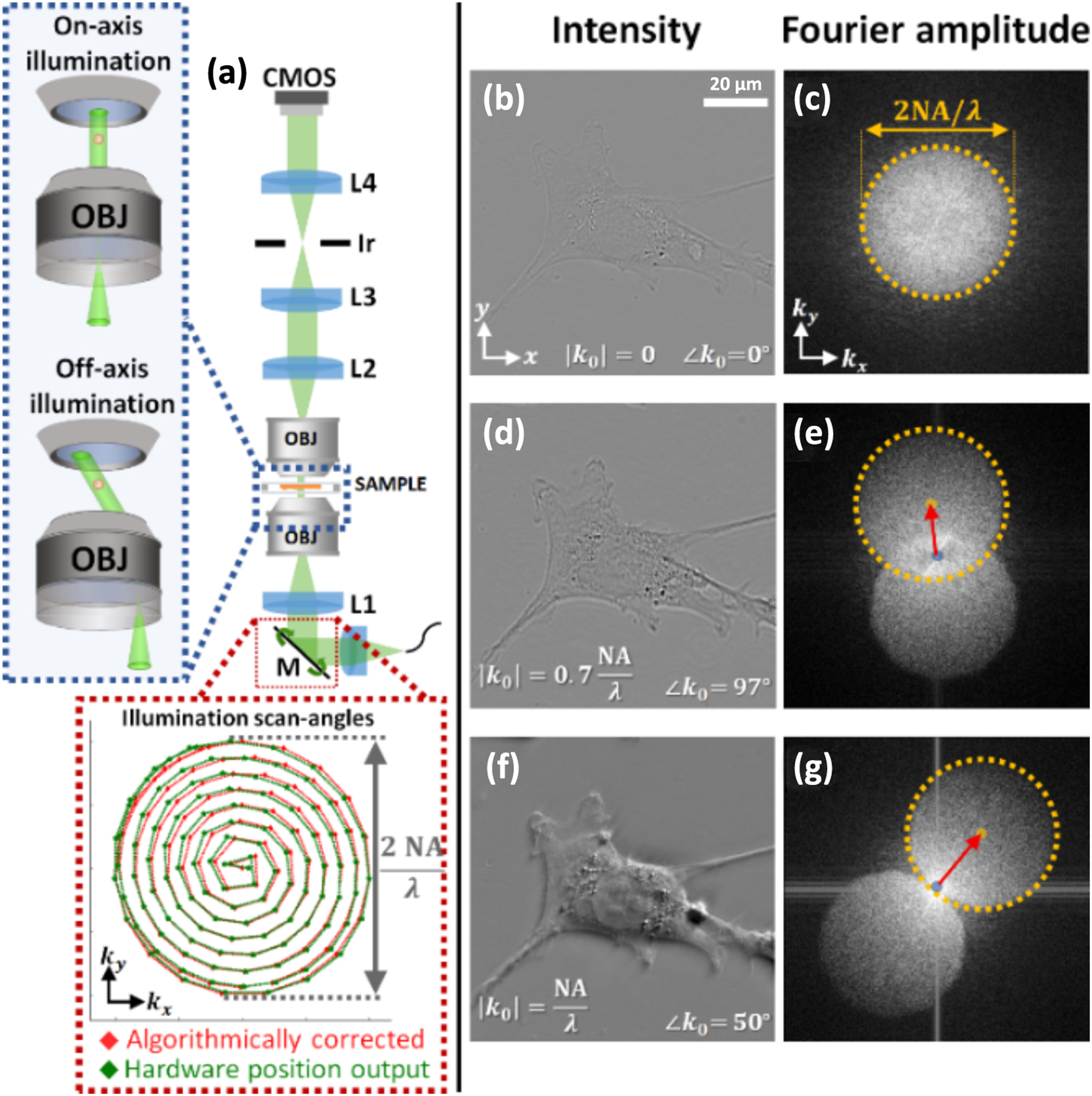
(a) Optical system design with illumination angle trajectories, comparing the raw position values outputted from the kinematic tilt mirror to that after algorithmic self-calibration. (b), (d), and (f) Raw intensity acquisitions and (c), (e), and (g) amplitudes of associated Fourier transforms, after illuminating the sample with varying angles.

B. Data Acquisition

The motorized kinematic mount for angle scanning was controlled via MATLAB and was programmed to scan the illumination through 120 angles along a spiral trajectory that fills the pupil [Fig. 1(a)]. As each scan point is reached, an Arduino board sends a trigger pulse to the sensor. Each image was captured with ~40 ms of integration time, resulting in a total acquisition time of 4.8 s. Reconstruction was performed with MATLAB running on a desktop computer equipped with Intel(R) Core(TM) i7-5960X CPU at 3.00GHz 64GB RAM CPU and NVidia’s GeForce GTX TitanX GPU. The total reconstruction time to complete 50 iterations of a 1200 × 1200 × 120 voxel volume was 20.3 h.

Figures 1(b), 1(d), and 1(f) and Fig. 1(c), 1(e), and 1(g) show the raw intensity measurements and associated Fourier magnitude, respectively, of a 3T3 fibroblast cell under different illumination angles. The Fourier transforms demonstrate that the spatial-frequency information is mostly contained within two circular regions in Fourier space, symmetrically positioned around the origin. This is expected for intensity-based imaging of weakly scattering objects with off-axis illumination [35,43] (see Supplement 1 for details).

C. Calibration of Illumination Angles

Our reconstruction requires precise knowledge of the illumination angles at the sample. Though illumination angles are outputted by the motorized kinematic mount, we experimentally found that such values did not have sufficient accuracy for satisfactory 3D RI reconstruction (likely due to system imperfections, sample-induced changes and misalignments). Thus, we instead use post-acquisition algorithmic angle-calibration as our means for precise angle measurement. We leverage previous developments in self-calibration to precisely estimate the incident illumination angles from the raw measurements [43]. Figures 1(c), 1(e), and 1(g) show that the illumination wavevectors ${\mathit{k}}_0^{\ell }$ can be estimated from the acquisitions’ Fourier transforms, since the center of the circles (illustrated with red arrows) correspond to the illumination angle (and its conjugate). For comparison, Fig. 1(a) shows the illumination angle values outputted by the hardware alongside those estimated by the self-calibration algorithm.

4. EXPERIMENTAL RESULTS

We experimentally demonstrate our method for 3D RI reconstruction of calibration objects and biological samples with varying amounts of multiple-scattering. We first image polystyrene beads for validation and then image a fibroblast cell, as an example of a weakly scattering sample. Finally, we look at multiple-scattering samples—C. elegans embryos and whole worm. Because all objects considered in this work are highly transparent with essentially no absorption, we show only the real component of the complex-valued RI reconstruction. Supplement 1 provides a comparison between the reconstruction quality obtained by our MSBP framework and the 1st Born reconstruction framework [32].

A. Polystyrene Microspheres

Figure 2 shows the 3D RI reconstruction of a conjoined pair of polystyrene spheres, mounted in immersion oil ($n\left(\lambda \right)=1.552$ at $\lambda =532\mathrm{n}\mathrm{m}$). The reconstruction used iterative step-size and regularization parameter set to $\alpha =6\times {10}^{-4}$ and $\beta =4\times {10}^{-4}$, respectively. Figure 2(a) shows a lateral slice through the center of the reconstruction volume. Figure 2(b) shows an axial slice taken across the horizontal dashed-white line in Fig. 2(a), and Fig. 2(c) shows a 3D rendered visualization of the reconstruction volume, clearly capturing the spherical geometry of the microspheres. A line-profile across a single microsphere [Fig. 2(d)] shows that the experimentally measured RI is in good agreement with the expected shape and RI of polystyrene ($n_s\left(\lambda \right)=1.598$ at $\lambda =532\mathrm{n}\mathrm{m}$) [44].

Fig. 2.

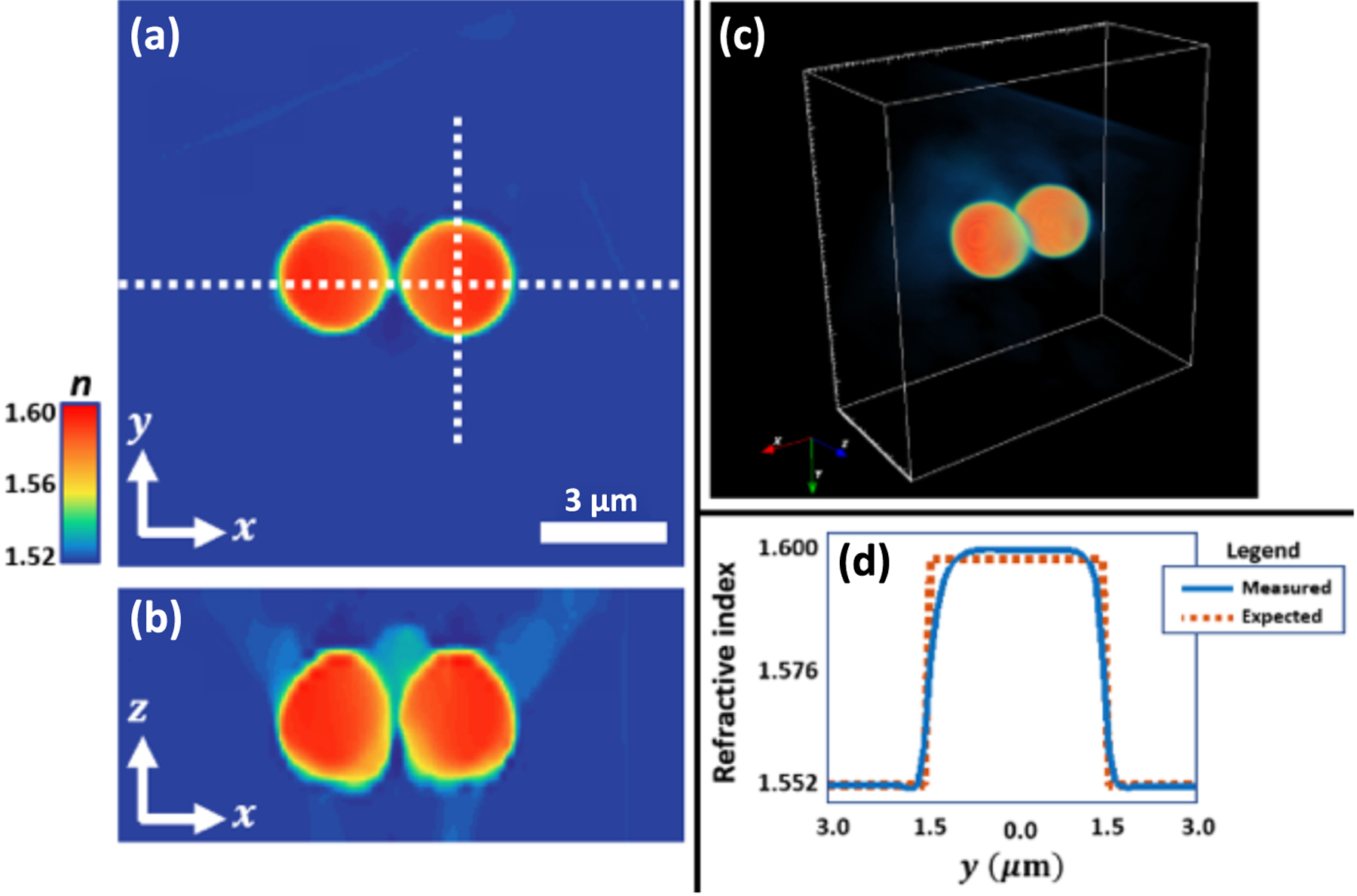
3D reconstruction of refractive index (RI) for two $3\mu \mathrm{m}$ diameter polystyrene microspheres $(n=1.598)$ in index-matched oil $(n=1.552)$. (a) Lateral $(x-y)$ slice, (b) axial $(x-z)$ slice, taken along the horizontal dashed line in (a), and (c) 3D rendering of the reconstructed microspheres. (d) Cross-cut of the refractive index along the vertical dashed line in (a) matches well with expected values from the sample.

B. Fibroblast Cells

We next demonstrate RI reconstruction (Visualization 1, Visualization 2, and Visualization 3, 700 × 700 × 40 voxels, $\alpha =4\times {10}^{-4},\beta =1\times {10}^{-5}$) of a weakly scattering fibroblast (3T3) cell, using our MSBP model. Figure 3 shows both grayscale and colored (for easier RI visualization after halo-removal [45]) lateral cross-sections at different depths through the reconstruction volume ($z=\mathrm{0.0,1.05}$, and $2.10\mu \mathrm{m}$, where $z=0.0\mu \mathrm{m}$ designates the attachment interface of the fibroblast cell to the coverslip). As adherent, migratory cells, fibroblast cells are known to form dynamic membrane protrusions [46]. These protrusions are clearly visualized in the reconstructed volume, with long filopodial extensions [indicated by yellow arrows in Fig. 3(c)] and broader lamellipodia and membrane ruffling at cell edges [red arrows in Figs. 3(a) and 3(c)]. Intracellular compartments also have strong contrast, notably the cell nucleus with the surrounding nuclear envelope and internal nucleoli. We show a zoom-in of this region in Fig. 3(e) to highlight the nuclear envelope (red arrows), internal nucleoli (yellow arrows), and outer region of optically-dense cellular structure.

Fig. 3.

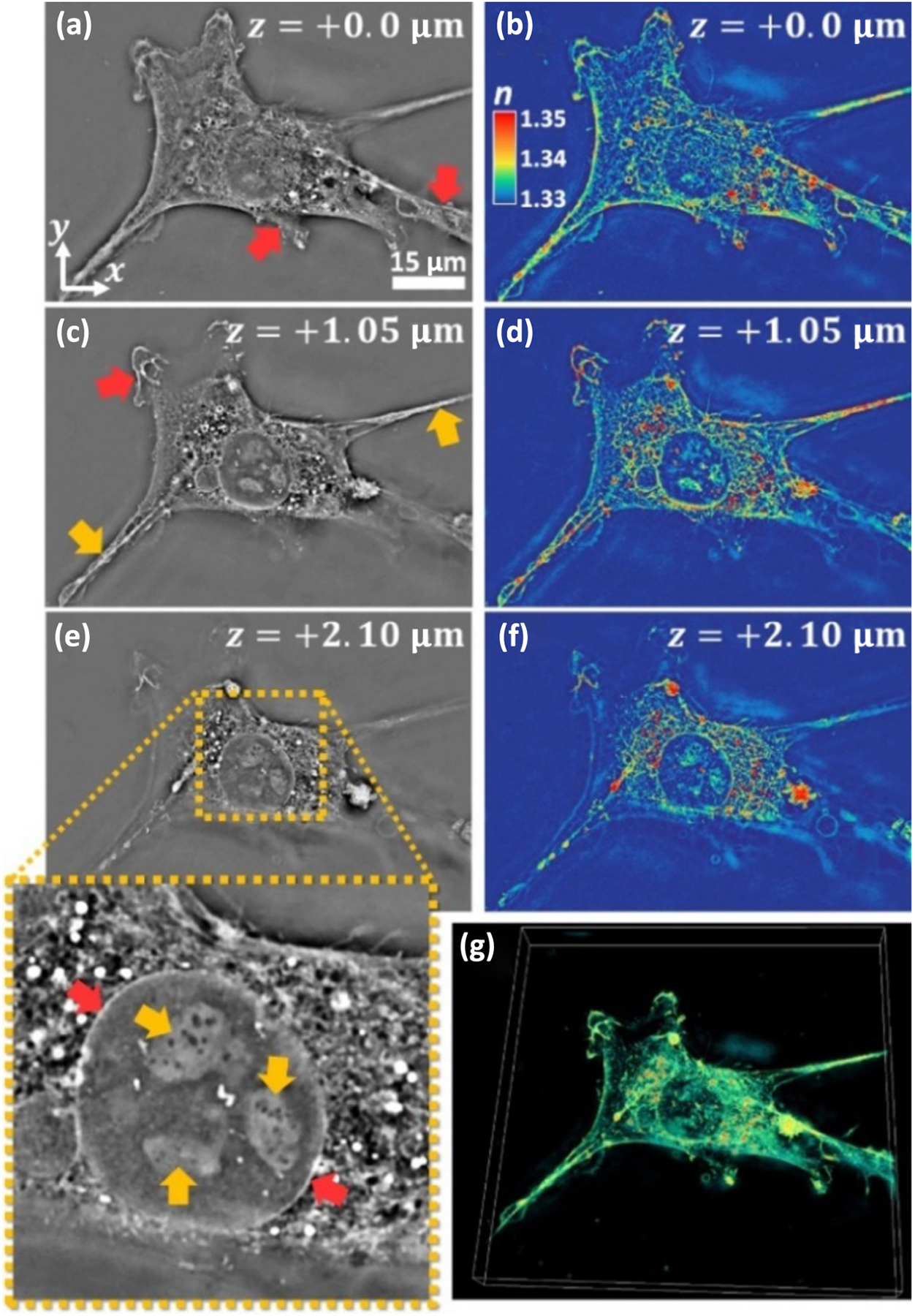
Lateral cross-sections (gray-scale and RGB color-coded) through the 3D RI reconstruction volume at axial positions of (a) and (b) $z=0.0\mu \mathrm{m}$, (c) and (d) $z=1.05\mu \mathrm{m}$, and (e) and (f) $z=2.10\mu \mathrm{m}$. (g) 3D rendering of the 3T3 cell RI.

The dense fibrous network within the cell is clearly visualized and exhibits a RI of 1.335–1.34 for the individual fiber tendrils. Intracellular lipids and nucleoli consistently demonstrate a RI > 1.35 and ~1.335, respectively, and the internuclear space shows a RI of ~1.33, matching closely the surrounding media. It has also been observed in previous works that the nuclear RI is lower than that of the general cell cytoplasm for various cell lines [7,47,48]. Figure 3(g) shows a tomographic rendering for easy identification of the 3D cell morphology.

C. Caenorhabditis elegans Embryos

Next, we image Caenorhabditis elegans (C. elegans) embryos captured at varying developmental stages [49]. Unlike the 3T3 cell, embryos are multicellular clusters and are, therefore, more condensed than any one individual cell. Thus, we expect such samples to exhibit more multiple-scattering. In Figs. 4(a)–4(c), we show the raw intensity measurements and associated Fourier amplitudes of the embryo clusters under three different illumination angles. Immediately, we see from Fig. 4(a) that the condensed internal structure within the C. elegans embryos results in significant intensity contrast even under orthogonal plane-wave illumination. This contrasts with the observations of the 3T3 fibroblast cell sample, which had virtually no intensity contrast under orthogonal illumination [see Fig. 1(b)]. This suggests that though the fibroblast cell can be modeled as weakly scattering, the C. elegans embryos cannot.

Fig. 4.

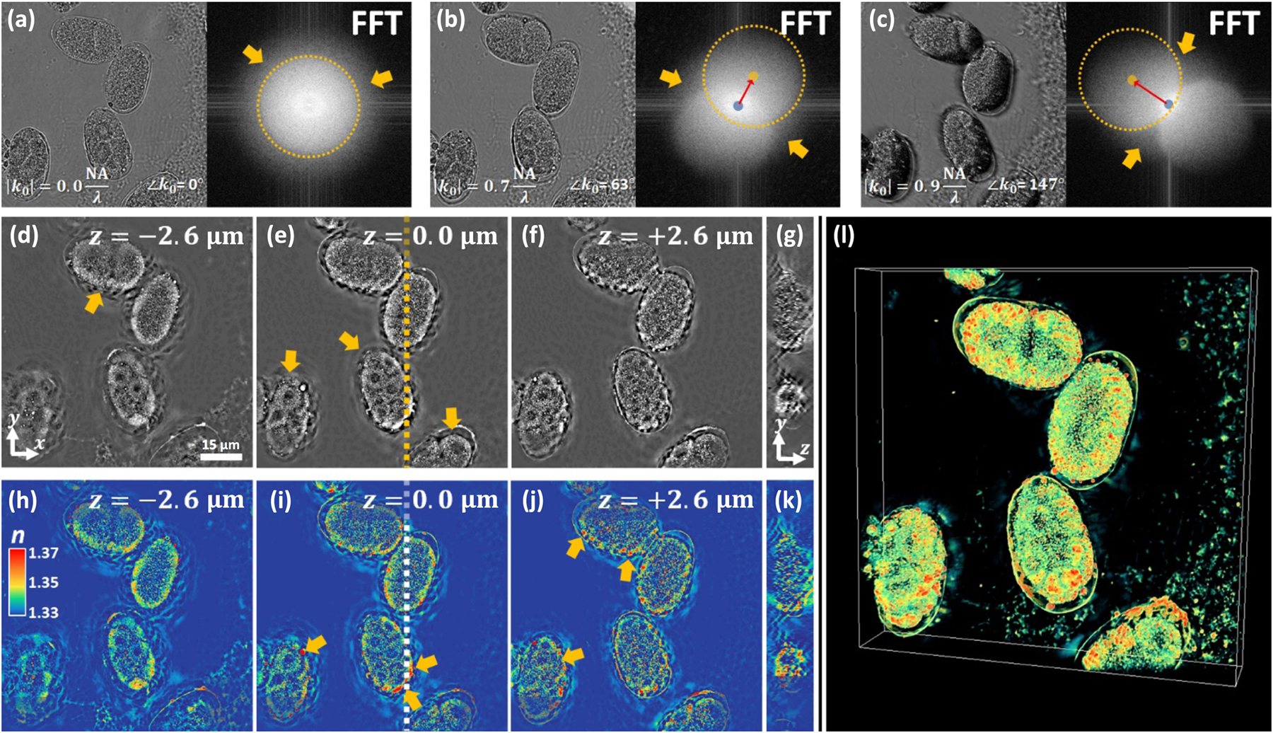
3D RI reconstruction of a C. elegans embryo cluster. (a)–(c) Raw intensity acquisitions at varying illumination angles, along with their Fourier transform amplitudes. (d)–(f) Lateral slices through the 3D reconstruction volume at axial positions $z=-\mathrm{2.6,0},+2.6\mu \mathrm{m}$. (g) Axial slice taken at the location indicated by the dashed line in (e). (h)–(k) Lateral and axial slices in (d)–(g) are redisplayed in RGB-color to facilitate easy visual inspection of refractive index. (l) 3D tomographic rendering of the embryo cluster.

More rigorous evidence of multiple-scattering comes from the Fourier transforms of the intensity acquisitions. As mentioned earlier and described in more detail in the Supplement 1, off-axis illumination of a weakly scattering sample results in intensity acquisitions where the spatial-frequencies lie within two circular regions in Fourier space. While the intensity spatial-frequency content of the 3T3 fibroblast cell [Figs. 1(c), 1(e), and 1(g)] was mainly contained in these circular regions, the C. elegans embryos show significant spatial-frequency content outside the two circles, as indicated by yellow arrows in Figs. 4(a)–4(c). This provides further evidence of multiple-scattering.

We show lateral slices from the 3D RI reconstruction (Visualization 4, Visualization 5, and Visualization 6, 1100 × 1100 × 120 voxels, $\alpha =6\times {10}^{-4}$ and $\beta =3.5\times {10}^{-4}$) of the embryo sample in both gray-scale [Figs. 4(d)–4(f)] and color-scale Figs. 4(h)–4(j), for three different depths ($z=-\mathrm{2.6,0}$, and $+2.6\mu \mathrm{m}$). Figures 4(g) and 4(k) show axial cross-sections, and Fig. 4(l) shows a 3D rendering. The features visualized in this 3D RI reconstruction fit well with their developmental stages, and individual cellular compartments can be identified. Yellow arrows in Fig. 4(d) and Fig. 4(e) indicate embryos visualized during their comma stage and general 8-cell to 26- cell stages, respectively. The axial cross-section in Fig. 4(g) demonstrates in 3D the embryos’ globular nature and heterogeneous composition, with RI values ranging from 1.33 to above 1.37, and shows a bulk RI increase towards the periphery of the embryos. Distinct eggshells are visualized encapsulating all embryos and demonstrate a moderately high RI ~1.35, which matches their known lipid-rich composition. Moreover, the lipoprotein complexes containing lipid and yolk proteins, localized between the embryo and eggshell, and show the highest RI as >1.375 [indicated with yellow arrows in Figs. 4(i) and 4(j)].

D. Whole Caenorhabditis elegans Worms

Our final experiment generates a high-resolution 3D RI reconstruction of a whole adult hermaphrodite C. elegans worm (Visualization 7, 1914 × 10408 × 118 voxels, $\alpha =4\times {10}^{-4},\left.\beta =4\times {10}^{-4}\right)$. Because the imaging objective’s field-of-view did not fit the whole worm, the final reconstruction volume was stitched together from 14 individually-reconstructed patches (details in Supplement 1). We note that unlike the embryos sample, the spatial-frequencies contained within the intensity measurements of the worm (shown in Supplement 1) do not contain any discernable symmetric circular regions. This indicates that the multiple-scattering in the worm sample dominates over the single-scattering and that the whole C. elegans worm is even more multiply-scattering than the embryos, as expected.

In Figs. 5(a) and 5(b), we show two lateral slices through the reconstruction volume at axial positions of $z=0.0$ and $-4.9\mu \mathrm{m}$, respectively. The major components of the reproductive and digestive systems are clearly identified and include the pharynx, intestine, gonads, spermathecal, and fertilized eggs [50]. Figure 5(c) presents an axial cross-section of the pharynx and clearly demonstrates the interior three-fold rotationally symmetric organization of the muscles and marginal cells around the pharyngeal lumen. Visualizing this morphology typically requires a heavily invasive preparation protocol (cross-sectional slicing through the C. elegans pharynx followed by electron microscopy) [51]. Figures 5(d) and 5(e) present a zoom-in of the worm’s mouth and pharyngeal tip at axial positions of $z=+2.42$ and $+5.19\mu \mathrm{m}$. Yellow arrows indicate E. coli bacteria, a food-source for the worm, present on the coverslip at the time of sample preparation. Red arrows indicate the cuticle surrounding the pharyngeal lumen and the buccal cavity, respectively.

Fig. 5.

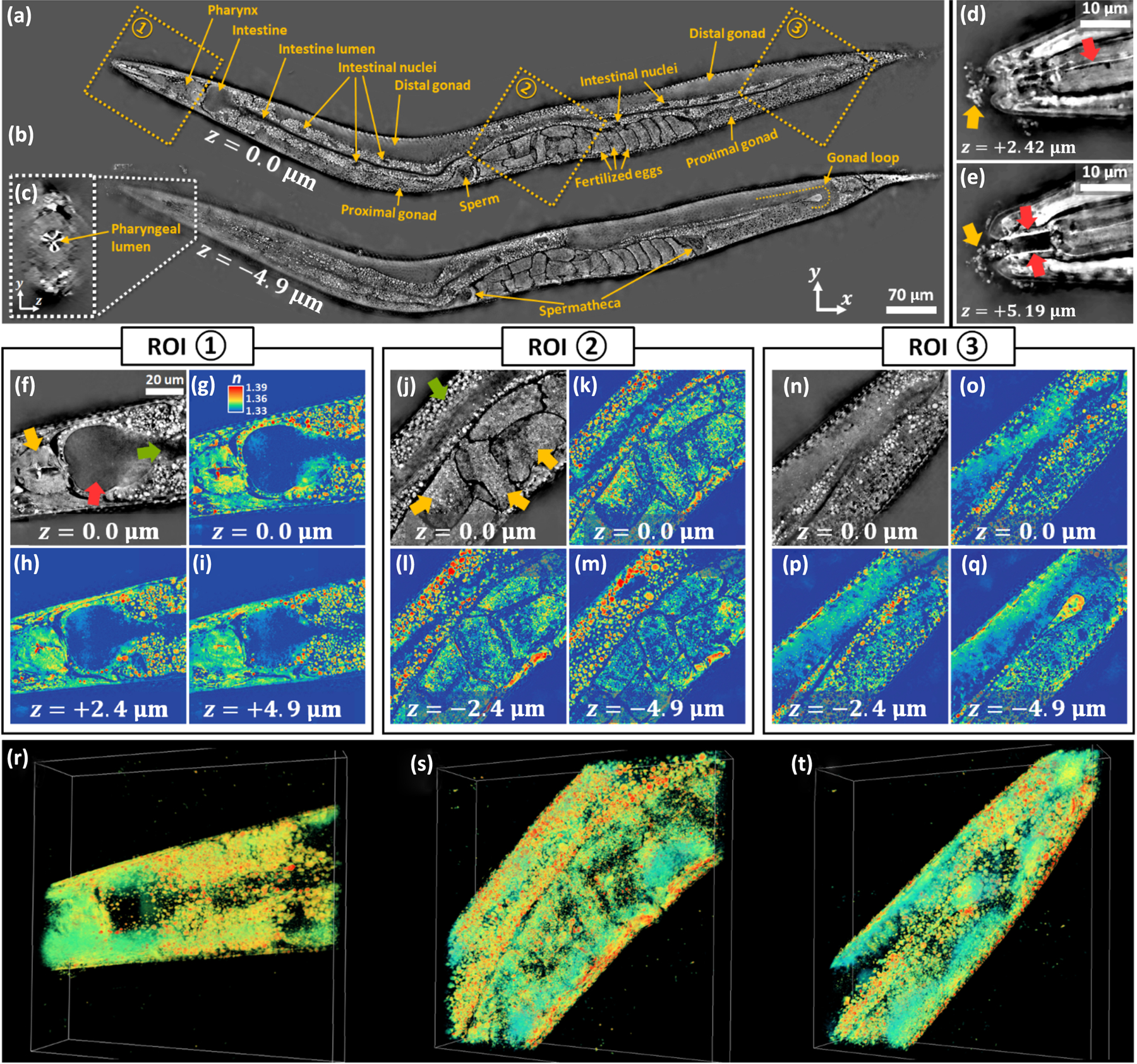
3D RI reconstruction of a whole C. elegans worm. (a) and (b) Lateral slices through the 3D reconstruction volume at axial positions $z=0,-4.9\mu \mathrm{m}$. Major components of the reproductive and digestive systems are labeled. (c) Axial slice through the pharynx. (d) and (e) Lateral slice zoom-ins of the worm’s head region at axial positions $z=+2.42,+5.19\mu \mathrm{m}$. Zoom-ins of the ROIs ①, ②, and ③ are shown in (f), (j), and (n), respectively. RGB-colored slices of the ROIs ①, ②, and ③ are shown with defocus in (g)–(i), (k)–(m), and (o)–(q), respectively. (r)–(t) 3D tomographic renderings of the ROIs ①, ②, and ③.

We outline three regions-of-interest (ROI) within Fig. 5(a), labeled as ①, ②, and ③, which highlight prominent structures within the C. elegans worm. Figure 5(f) shows a zoom of the ROI ① and qualitatively highlights the features pertaining to the pharynx-bulb, intestinal cavity, and the start of the intestinal lumen, as indicated by the yellow, red, and green arrows, respectively. Figure 5(j) shows a zoom-in of the ROI ② and depicts fertilized eggs and the distal gonad, as indicated by the yellow and green arrows, respectively. Figure 5(n) shows a zoom of the ROI ③ at the tail-end of the worm and highlights the distal and proximal gonads. To quantitatively visualize the worm’s 3D biological RI, we present RBG-colored cross-sectional images of all ROIs at various axial positions. Figures 5(g)–5(i) show quantitative RI cross-sections of the ROI ① at $z=0.0\mu \mathrm{m}$, $+2.4\mu \mathrm{m}$, and $+4.9\mu \mathrm{m}$, respectively. Figures 5(k)–5(m) and Fig. 5(o)–5(q) show quantitative RI cross-sections of the ROI ② and ③, respectively, at $z=0.0,-2.4$, and $-4.9\mu \mathrm{m}$. The bulk tissue of the pharynx and gonads are of relatively consistent RI ~1.35. The fertilized eggs, however, demonstrate high heterogeneity (corroborated by DIC imaging) with RI values ranging from 1.335 to 1.35, and regions with high density of lipid droplets, such as the intestine or the proximal gonads, consist of the most variable scattering. Individual lipid droplets can demonstrate RI values as high as 1.40 and are often directly surrounded by features of low RI, ~1.335. Figures 5(r)–5(t) show 3D tomographic visualizations of the ROIs ①, ②, and ③, respectively.

5. DISCUSSION

This work demonstrates a cost-effective and simple optical hardware system that uses computational imaging for biological imaging problems where no analytical solution exists, as is the case with multiple-scattering. This comes at a cost of higher computational requirements than standard ODT. In this work, every angled illumination corresponds to two passes through all layers of the reconstruction volume, which increments the sample’s predicted 3D RI one step along its convergence curve. Factors such as increasing the number of acquisitions (to increase the likelihood of correct convergence for the reconstruction) or the resolution of the reconstruction volume further slow the computation. To address this, future work will leverage the recent advent of big-data processing via GPU acceleration or cloud-computing to significantly reduce reconstruction times.

Another interesting extension would be to explore the maximum resolution achievable using the introduced framework. Previous works have demonstrated that multiple-scattering, if considered appropriately, can significantly improve a microscope’s resolving power to beyond the diffraction limit [34,37,38]. However, this capability for resolution enhancement is difficult to quantify because it depends on the multiple-scattering characteristics of the object, which are generally unknown. Furthermore, strongly scattering objects typically also exhibit strong back-scattering, which is not mathematically treated in our MSBP model. Thus, future work will also explore strategies to incorporate back-scattering into our imaging model as well as to estimate the maximum attainable resolution, based on inferences of the sample’s multiple-scattering characteristics.

6. CONCLUSION

In this work, we have introduced a new computational technique that uses the multi-slice beam-propagation model to reconstruct 3D RI with high-resolution, even in multiply-scattering samples. Compared to the standard ODT techniques, our method offers two key advantages: (1) intensity-only acquisitions enable phase-stable and speckle-free measurements with a dramatically simpler and cheaper optical system and (2) we impose no constraints upon the sample to be weakly scattering, such that suitable samples need not be limited to a sparse distribution of individual cells. This opens up 3D RI microscopy to the more general class of biological samples that include dense cell-clusters or multicellular organisms.

We experimentally demonstrated our method by first reconstructing 3D RI of 3T3 fibroblast cells and C. elegans embryos, as examples of single-cell (weakly scattering) and multi-cell cluster (multiple-scattering) samples, respectively. In both cases, the MSBP model enabled high-fidelity and robust RI reconstruction. Our final demonstration was the 3D RI reconstruction of a whole C. elegans worm as an example of the applicability of this technique to whole multicellular organisms, even in the presence of multiple-scattering. To the best of our knowledge, this is the first demonstration of high-resolution (NA > 1.0) intensity-based 3D RI reconstruction of multiple-scattering biological samples. Due to the simplicity of the introduced optical system, easy hardware additions can be implemented to adapt the system to existing fluorescent microscopes and enable 3D multimodal imaging [47,52,53].

Download video file ^{(61.4MB, mp4)}

Download video file ^{(24.3MB, mp4)}

Download video file ^{(40.4MB, mp4)}

Download video file ^{(8.6MB, mp4)}

Download video file ^{(23.3MB, mp4)}

Download video file ^{(8.2MB, mp4)}

Download video file ^{(11.4MB, mp4)}

REFERENCES

- 1.Ross DT, Scherf U, Eisen MB, Perou CM, Rees C, Spellman P, Iyer V, Jeffrey SS, Van de Rijn M, and Waltham M, “Systematic variation in gene expression patterns in human cancer cell lines,” Nat. Genet 24, 227–235 (2000) [DOI] [PubMed] [Google Scholar]
- 2.Rustom A, Saffrich R, Markovic I, Walther P, and Gerdes H-H, “Nanotubular highways for intercellular organelle transport,” Science 303, 1007–1010 (2004). [DOI] [PubMed] [Google Scholar]
- 3.Okuda M, Li K, Beard MR, Showalter LA, Scholle F, Lemon SM, and Weinman SA, “Mitochondrial injury, oxidative stress, and antioxidant gene expression are induced by hepatitis C virus core protein,” Gastroenterology 122, 366–375 (2002). [DOI] [PubMed] [Google Scholar]
- 4.Rizzuto R, Brini M, Pizzo P, Murgia M, and Pozzan T, “Chimeric green fluorescent protein as a tool for visualizing subcellular organelles in living cells,” Curr. Biol 5, 635–642 (1995). [DOI] [PubMed] [Google Scholar]
- 5.Choi W, Fang-Yen C, Badizadegan K, Oh S, Lue N, Dasari RR, and Feld MS, “Tomographic phase microscopy,” Nat. Methods 4, 717–719 (2007). [DOI] [PubMed] [Google Scholar]
- 6.Lauer V, “New approach to optical diffraction tomography yielding a vector equation of diffraction tomography and a novel tomographic microscope,” J. Microsc 205, 165–176 (2002) [DOI] [PubMed] [Google Scholar]
- 7.Sung Y, Choi W, Fang-Yen C, Badizadegan K, Dasari RR, and Feld MS, “Optical diffraction tomography for high resolution live cell imaging,” Opt. Express 17, 266–277 (2009). [DOI] [PMC free article] [PubMed] [Google Scholar]
- 8.Fiolka R, Wicker K, Heintzmann R, and Stemmer A, “Simplified approach to diffraction tomography in optical microscopy,” Opt. Express 17, 12407–12417 (2009). [DOI] [PubMed] [Google Scholar]
- 9.Lee S, Kim K, Mubarok A, Panduwirawan A, Lee K, Lee S, Park H, and Park Y, “High-resolution 3-D refractive index tomography and 2-D synthetic aperture imaging of live phytoplankton,” J. Opt. Soc. Korea 18, 691–697 (2014). [Google Scholar]
- 10.Kim T, Zhou R, Mir M, Babacan SD, Carney PS, Goddard LL, and Popescu G, “White-light diffraction tomography of unlabelled live cells,” Nat. Photonics 8, 256–263 (2014). [Google Scholar]
- 11.Nguyen TH, Kandel ME, Rubessa M, Wheeler MB, and Popescu G, “Gradient light interference microscopy for 3D imaging of unlabeled specimens,” Nat. Commun 8, 210 (2017). [DOI] [PMC free article] [PubMed] [Google Scholar]
- 12.Park Y, Diez-Silva M, Popescu G, Lykotrafitis G, Choi W, Feld MS, and Suresh S, “Refractive index maps and membrane dynamics of human red blood cells parasitized by Plasmodium falciparum,” Proc. Natl. Acad. Sci. USA 105, 13730–13735 (2008). [DOI] [PMC free article] [PubMed] [Google Scholar]
- 13.Eldridge WJ, Sheinfeld A, Rinehart MT, and Wax A, “Imaging deformation of adherent cells due to shear stress using quantitative phase imaging,” Opt. Lett 41, 352–355 (2016). [DOI] [PubMed] [Google Scholar]
- 14.Shaked NT, Satterwhite LL, Bursac N, and Wax A, “Whole-cell-analysis of live cardiomyocytes using wide-field interferometric phase microscopy,” Biomed. Opt. Express 1, 706–719 (2010). [DOI] [PMC free article] [PubMed] [Google Scholar]
- 15.Jung J, Kim K, Yoon J, and Park Y, “Hyperspectral optical diffraction tomography,” Opt. Express 24, 2006–2012 (2016). [DOI] [PubMed] [Google Scholar]
- 16.Kou SS and Sheppard CJ, “Image formation in holographic tomography: high-aperture imaging conditions,” Appl. Opt 48, H168–H175 (2009). [DOI] [PubMed] [Google Scholar]
- 17.Habaza M, Gilboa B, Roichman Y, and Shaked NT, “Tomographic phase microscopy with 180 rotation of live cells in suspension by holographic optical tweezers,” Opt. Lett 40, 1881–1884 (2015). [DOI] [PubMed] [Google Scholar]
- 18.Simon B, Debailleul M, Houkal M, Ecoffet C, Bailleul J, Lambert J, Spangenberg A, Liu H, Soppera O, and Haeberlé O, “Tomographic diffractive microscopy with isotropic resolution,” Optica 4, 460–463 (2017). [Google Scholar]
- 19.Devaney A, “Inverse-scattering theory within the Rytov approximation,” Opt. Lett 6, 374–376 (1981). [DOI] [PubMed] [Google Scholar]
- 20.Lin F and Fiddy M, “The Born-Rytov controversy: I. Comparing analytical and approximate expressions for the one-dimensional deterministic case,” J. Opt. Soc. Am. A 9, 1102–1110 (1992). [Google Scholar]
- 21.Chen B and Stamnes JJ, “Validity of diffraction tomography based on the first Born and the first Rytov approximations,” Appl. Opt 37, 2996–3006 (1998). [DOI] [PubMed] [Google Scholar]
- 22.Wolf E, “Three-dimensional structure determination of semi-transparent objects from holographic data,” Opt. Commun 1, 153–156 (1969). [Google Scholar]
- 23.Cotte Y, Toy F, Jourdain P, Pavillon N, Boss D, Magistretti P, Marquet P, and Depeursinge C, “Marker-free phase nanoscopy,” Nat. Photonics 7, 113–117 (2013). [Google Scholar]
- 24.Kim K, Yoon H, Diez-Silva M, Dao M, Dasari RR, and Park Y, “High-resolution three-dimensional imaging of red blood cells parasitized by Plasmodium falciparum and in situ hemozoin crystals using optical diffraction tomography,” J. Biomed. Opt 19, 011005 (2014). [DOI] [PMC free article] [PubMed] [Google Scholar]
- 25.Chowdhury S, Eldridge WJ, Wax A, and Izatt J, “Refractive index tomography with structured illumination,” Optica 4, 537–545 (2017). [DOI] [PMC free article] [PubMed] [Google Scholar]
- 26.Maleki MH and Devaney AJ, “Phase-retrieval and intensity-only reconstruction algorithms for optical diffraction tomography,” J. Opt. Soc. Am. A 10, 1086–1092 (1993). [Google Scholar]
- 27.Yang G-Z, Dong B-Z, Gu B-Y, Zhuang J-Y, and Ersoy OK, “Gerchberg-Saxton and Yang-Gu algorithms for phase retrieval in a nonunitary transform system: a comparison,” Appl. Opt 33, 209–218 (1994). [DOI] [PubMed] [Google Scholar]
- 28.Kamilov US, Liu D, Mansour H, and Boufounos PT, “A recursive Born approach to nonlinear inverse scattering,” IEEE Signal Process. Lett 23, 1052–1056 (2016). [Google Scholar]
- 29.Ancora D, Di Battista D, Giasafaki G, Psycharakis SE, Liapis E, Ripoll J, and Zacharakis G, “Optical projection tomography via phase retrieval algorithms,” Methods 136, 81–89 (2018). [DOI] [PubMed] [Google Scholar]
- 30.Froustey E, Bostan E, Lefkimmiatis S, and Unser M, “Digital phase reconstruction via iterative solutions of transport-of-intensity equation,” in 13th Workshop on Information Optics WIO) (IEEE, 2014), pp. 1–3. [Google Scholar]
- 31.Liu H-Y, Liu D, Mansour H, Boufounos PT, Waller L, and Kamilov US, “SEAGLE: sparsity-driven image reconstruction under multiple scattering,” IEEE Trans. Comput. Imag 4, 73–86 (2018). [Google Scholar]
- 32.Horstmeyer R, Chung J, Ou X, Zheng G, and Yang C, “Diffraction tomography with Fourier ptychography,” Optica 3, 827–835 (2016). [DOI] [PMC free article] [PubMed] [Google Scholar]
- 33.Kamilov US, Papadopoulos IN, Shoreh MH, Goy A, Vonesch C, Unser M, and Psaltis D, “Optical tomographic image reconstruction based on beam propagation and sparse regularization,” IEEE Trans. Comput. Imag 2, 59–70 (2016). [Google Scholar]
- 34.Tian L and Waller L, “3D intensity and phase imaging from light field measurements in an LED array microscope,” Optica 2, 104–111 (2015). [Google Scholar]
- 35.Ling R, Tahir W, Lin H-Y, Lee H, and Tian L, “High-throughput intensity diffraction tomography with a computational microscope,” Biomed. Opt. Express 9, 2130–2141 (2018). [DOI] [PMC free article] [PubMed] [Google Scholar]
- 36.Chen M, Tian L, and Waller L, “3D differential phase contrast microscopy,” Biomed. Opt. Express 7, 3940–3950 (2016). [DOI] [PMC free article] [PubMed] [Google Scholar]
- 37.Park J-H, Park C, Yu H, Park J, Han S, Shin J, Ko SH, Nam KT, Cho Y-H, and Park Y, “Subwavelength light focusing using random nanoparticles,” Nat. Photonics 7, 454–458 (2013). [Google Scholar]
- 38.Belkebir K, Chaumet PC, and Sentenac A, “Influence of multiple scattering on three-dimensional imaging with optical diffraction tomography,” J. Opt. Soc. Am. A 23, 586–595 (2006). [DOI] [PubMed] [Google Scholar]
- 39.Van Roey J, Van der Donk J, and Lagasse P, “Beam-propagation method: analysis and assessment,” J. Opt. Soc. Am 71, 803–810 (1981). [Google Scholar]
- 40.Chung Y and Dagli N, “An assessment of finite difference beam propagation method,” IEEE J. Quantum Electron 26, 1335–1339 (1990). [Google Scholar]
- 41.Maiden AM, Humphry MJ, and Rodenburg J, “Ptychographic transmission microscopy in three dimensions using a multi-slice approach,” J. Opt. Soc. Am. A 29, 1606–1614 (2012). [DOI] [PubMed] [Google Scholar]
- 42.Yeh L-H, Dong J, Zhong J, Tian L, Chen M, Tang G, Soltanolkotabi M, and Waller L, “Experimental robustness of Fourier ptychography phase retrieval algorithms,” Opt. Express 23, 33214–33240 (2015). [DOI] [PubMed] [Google Scholar]
- 43.Eckert R, Phillips ZF, and Waller L, “Efficient illumination angle self-calibration in Fourier ptychography,” Appl. Opt 57, 5434–5442 (2018). [DOI] [PubMed] [Google Scholar]
- 44.Sultanova N, Kasarova S, and Nikolov I, “Dispersion properties of optical polymers,” Acta Phys. Pol. A 116, 585–587 (2009). [Google Scholar]
- 45.Kandel ME, Fanous M, Best-Popescu C, and Popescu G, “Real-time halo correction in phase contrast imaging,” Biomed. Opt. Express 9, 623–635 (2018). [DOI] [PMC free article] [PubMed] [Google Scholar]
- 46.Small JV, Stradal T, Vignal E, and Rottner K, “The lamellipodium: where motility begins,” Trends Cell Biol. 12, 112–120 (2002). [DOI] [PubMed] [Google Scholar]
- 47.Chowdhury S, Eldridge WJ, Wax A, and Izatt JA, “Structured illumination microscopy for dual-modality 3D sub-diffraction resolution fluorescence and refractive-index reconstruction,” Biomed. Opt. Express 8, 5776–5793 (2017). [DOI] [PMC free article] [PubMed] [Google Scholar]
- 48.Schürmann M, Scholze J, Müller P, Guck J, and Chan CJ, “Cell nuclei have lower refractive index and mass density than cytoplasm,” J. Biophoton 9, 1068–1076 (2016). [DOI] [PubMed] [Google Scholar]
- 49.Sulston JE, Schierenberg E, White JG, and Thomson J, “The embryonic cell lineage of the nematode Caenorhabditis elegans,” Dev. Biol 100, 64–119 (1983). [DOI] [PubMed] [Google Scholar]
- 50.White JG, Southgate E, Thomson JN, and Brenner S, “The structure of the nervous system of the nematode Caenorhabditis elegans,” Philos. Trans. R. Soc. B 314, 1–340 (1986). [DOI] [PubMed] [Google Scholar]
- 51.Mango SE, The C Elegans Pharynx: a Model for Organogenesis (2007). [DOI] [PMC free article] [PubMed]
- 52.Park Y, Popescu G, Badizadegan K, Dasari RR, and Feld MS, “Diffraction phase and fluorescence microscopy,” Opt. Express 14, 8263–8268 (2006) [DOI] [PubMed] [Google Scholar]
- 53.Kim K, Park WS, Na S, Kim S, Kim T, Heo WD, and Park Y, “Correlative three-dimensional fluorescence and refractive index tomography: bridging the gap between molecular specificity and quantitative bioimaging,” Biomed. Opt. Express 8, 5688–5697 (2017). [DOI] [PMC free article] [PubMed] [Google Scholar]
Associated Data
This section collects any data citations, data availability statements, or supplementary materials included in this article.