Cross-evaluation of E. coli’s operon structures via a whole-cell model suggests alternative cellular benefits for low- versus high-expressing operons

Summary

Many bacteria use operons to coregulate genes, but it remains unclear how operons benefit bacteria. We integrated E. coli’s 788 polycistronic operons and 1,231 transcription units into an existing whole-cell model, and found inconsistencies between the proposed operon structures and the RNA-Seq read counts that the model was parameterized from. We resolved these inconsistencies through iterative, model-guided corrections to both datasets, including the correction of RNA-Seq counts of short genes that were misreported as zero by existing alignment algorithms. The resulting model suggested two main modes by which operons benefit bacteria. For 86% of low-expression operons, adding operons increased the coexpression probabilities of their constituent proteins, while for 92% of high-expression operons, adding operons resulted in more stable expression ratios between the proteins. These simulations underscored the need for further experimental work on how operons reduce noise and synchronize both the expression timing and the quantity of constituent genes. A record of this paper’s Transparent Peer Review process is included in the Supplemental Information.

eTOC blurb

To explore how operons benefit bacteria, Sun et al. update an E. coli whole-cell model to account for operons. In the process, they find inconsistencies between input datasets which they resolve through model-guided corrections. Simulations suggest that operons increase co-expression probabilities for low-expression genes, while stabilizing stoichiometries for high-expression genes.

Graphical Abstract

Introduction

Coregulation of genes through operons is a key mechanism that many organisms, mostly bacteria, have evolved to organize their transcriptomes. Since the discovery of the lac operon in E. coli¹, many theories have been proposed on what selective advantages operons would bring to bacteria, as opposed to placing the same genes under the control of identical but independent promoters. Some have suggested that operons evolved solely because they facilitate simultaneous horizontal transfer of functionally related genes by placing them close together on the genome^2,3 (the “selfish” operon theory); other suggestions include that operons provide a more information-efficient way to coregulate genes compared to alternative methods⁴, facilitate easier complexation between protein subunits^5,6, or decrease gene expression noise⁷.

In the context of this debate, it should be noted that there is great diversity in the features of operons that have been characterized so far in bacterial genomes. In E. coli, for example, many operons consist of genes that are heavily regulated and only function under specific environments, with the lac operon being a prime example. However, many other operons consist of genes that are constitutively expressed, such as the spc operon, which consists of ten genes encoding for ribosomal proteins⁸. Some E. coli operons are “canonical” in the sense that they contain a single promoter and a single transcription terminator, and thus always express all genes in the operon as a single, contiguous transcription unit. Other operons have more complex transcription unit structures that include internal promoters and/or terminators, and can transcribe multiple mRNA isoforms that span different combinations of genes within the operon^9–11. Given this diversity, it is unlikely that a single mechanism would explain the utility of all operons in E. coli, let alone all bacterial species.

In this work, we use the E. coli whole-cell model to investigate the role of operons in the regulation of gene expression dynamics. The long-term goal of the E. coli Whole-Cell Modeling Project is to build a mechanistic simulation of an E. coli cell that takes into account the known functions of all genes and molecules¹², as once proposed by Francis Crick¹³. The key innovation that enabled the building of a model of such scale was the division of the cell into multiple, independent modules that each represent a particular biological process within the cell (metabolism, transcription, translation, etc.). Each module was then represented with a “submodel” that uses a mathematical framework that is most appropriate for the corresponding biological process, given the properties of the process itself and the level of knowledge or data we currently have about its dynamics (See STAR Methods for more details on whole-cell modeling concepts). Three years ago, a first version of the E. coli whole-cell model was reported, which integrated more than 19,000 parameters collected from hundreds of heterogeneous data sources, and mathematically represented the functions of 43% of the well-annotated genes of E. coli¹⁴. Whole-cell models have produced simulation outputs that were validated by experiments and have made predictions on emergent properties of the cells being modeled^14–17.

Because of the inherent noisiness of bacterial gene expression and the resulting heterogeneity between individual bacterial cells, it has been challenging to understand the effects of operon structures via experimental methods. Thus, many studies that have previously explored this question have instead made use of mathematical models that simulate the stochastic expression of genes from bacterial promoters at the single-cell level. However, these studies either chose to model one specific operon¹⁸, or hypothetical operons with generalized parameters^7,19,20, belying the aforementioned diversity in how operons operate within these cells. The E. coli whole-cell model allows us to quantitatively probe the gene expression dynamics for virtually all of the protein-coding operons in E. coli with their own specific parameters, providing a unique opportunity to explore this problem theoretically in both great breadth and detail. While experimental validation would still be necessary, this modeling approach allows us to run simulated experiments that would be prohibitively costly to conduct in a similar scale in an actual experimental setting, while also providing us with data on the fine-grained dynamics of gene expression at the level of individual cells that would not be possible to measure experimentally with the current technology. Consequently, by using the whole-cell model to explore this question, we are able to propose broad, genome-scale hypotheses on the utility of bacterial operons.

In order to use the E. coli whole-cell model for this particular purpose, however, we first need to update the model to account for E. coli’s operon structures. In the first published version of the whole-cell model¹⁴, it was assumed that each gene in E. coli is transcribed as its own, monocistronic transcription unit, largely because of difficulties in acquiring the experimental data that was needed to parameterize a model with polycistronic transcripts. More specifically, the model used two experimentally measured parameters to determine how frequently each mRNA species should be transcribed: the RNA-Seq read counts of the mRNA, and its degradation half-life (See STAR Methods for more details on the transcription submodel). Both of these numbers, however, are usually only reported at the level of individual genes and not at the level of longer polycistronic transcription units, due to technical limitations in the respective experimental methods used to acquire these data. Conventional short-read RNA-Seq protocols require the sample RNA to be digested into fragments that are shorter than most genes before they are sequenced, which leads to the loss of long-range context that was present in the original sample^21,22, while degradation half-lives of mRNAs were taken from an experiment that used microarrays²³, whose resolution is similarly limited to the gene level. Long-read RNA sequencing is a promising development that may be able to provide these types of measurements for polycistronic transcripts^24,25, but the currently available data for E. coli is not comprehensive enough to be used for the whole-cell model.

While precise quantification of polycistronic transcripts at the omics level remains a challenge, our knowledge of operons and their transcription unit structures in the E. coli genome has expanded greatly since the discovery of the lac operon. Over many years, the curators at RegulonDB have compiled a list of all operons and transcription units that have been characterized so far in the E. coli genome²⁶, and this compilation has been hosted and expanded as part of the EcoCyc database²⁷. According to this list, we now have evidence that E. coli groups its 4,307 mRNA-encoding genes into 2,569 operons. 788 of these operons are polycistronic and are responsible for transcribing 2,526 (~59%) of the mRNA-encoding genes with 1,231 transcription units that span distinct combinations of genes. 521 of these polycistronic operons are canonical operons where all constituent genes are transcribed as a single transcription unit, while 267 operons have more complicated transcription unit structures. In addition to this list of transcription units curated by RegulonDB/EcoCyc, advanced RNA-Seq techniques were recently used to measure the degradation half-lives of a small subset of polycistronic transcripts at the level of the entire mRNA²⁸, which provides us with some of the parameters necessary to model the degradation of these RNAs at the transcript level.

Thus, while direct measurement of all required parameters remains difficult, the availability of these additional datasets provides us with a starting point to build an updated version of the whole-cell model that accounts for operons (Figure 1A, “Heterogeneous data”). These additional datasets, combined with the data used by the first version of the whole-cell model^14,23,29,30, are used to theoretically estimate a set of parameters that can describe gene expression at the level of individual transcription units, rather than individual genes (Figure 1A, “Simulation parameters”). These updated values populate the transcription submodel of the whole-cell model, which has been entirely reconfigured to handle the transcription of polycistronic mRNAs that cover multiple genes (Figure 1A, “Transcription submodel”). The rebuilt transcription submodel is connected with the other submodels to build the updated whole-cell model (Figure 1A, “E. coli whole-cell model”), which produces detailed simulations of E. coli growth while accounting for operons (Figure 1A, “Simulation outputs”). Figure 1B compares selected simulation outputs to illustrate the overall impact of this model update, with a focus on the expression of genes constituting the frdABCD operon, where each gene encodes for one of the four subunits of the fumarate reductase enzyme complex³¹. The original version of the model transcribed these four genes independently from each other as their own, monocistronic mRNAs (Figure 1B, left). The updated version transcribes the four genes of the operon as a single transcription unit, which then serves as a template to translate all four protein subunits, resulting in a more coordinated expression of the four proteins (Figure 1B, right).

Figure 1.

Additional experimental data gathered from multiple, heterogeneous sources were incorporated into the E. coli whole-cell model to simulate cells that transcribe polycistronic mRNAs. (A) Schematic representation of the data curation process that was used to update the whole-cell model. We incorporated additional data on E. coli’s transcription units into the existing whole-cell model, iteratively identified inconsistencies between the input data using the simulation outputs, and made guided corrections to the input data, which were verified through comparisons with independent data, to finalize an updated version of the E. coli whole-cell model that transcribes polycistronic mRNAs. (B) Comparison of the simulated expression dynamics of the frdABCD operon before and after the update.

Similar to our experience in building the original version of the E. coli whole-cell model, however, we find that a naïve integration of these additional datasets into the model results in unstable simulations that highlight inconsistencies between the input datasets. As the whole-cell model integrates heterogeneous experimental data that contain varying degrees of errors into a cohesive, unified model, the resulting model outputs can reveal conflicts between these datasets that would not be apparent when these datasets are analyzed independently from each other. In previous works, we had shown that we can use the whole-cell model’s outputs to identify these conflicts between input datasets and make model-guided corrections to these datasets to make them more cross-consistent – a process that we call “deep curation”^12,14 (See STAR Methods for more details on deep curation). In this work, we similarly use the outputs from the updated whole-cell model to make guided corrections to the transcription unit structures curated by RegulonDB/EcoCyc and the RNA-Seq read counts (Figure 1A). To verify these corrections, we use data from Rend-seq³², a recently developed RNA sequencing technique that can identify transcription start and end sites, and data from Dar and Sorek³³, which provide a list of E. coli operons whose mRNAs undergo nonuniform degradation.

The details on how we iteratively used the model’s outputs to make guided adjustments to the input data, with the goal of improving the data’s cross-consistency and the overall coherence of the simulated outputs, will be the focus of the first half of this work (Figure 1A). The second half will describe the final, conflict-resolved version of the updated model that includes operon structures and compare its outputs against the original version of the model that does not use operons (Figure 1B is a preview). Our simulated comparisons suggest two major modes by which operons can benefit bacterial cells. For low-expression genes, operons increase the probability that their constituent genes are co-expressed both at the mRNA and protein levels, which has an impact on the phenotypic properties of the colony if the genes are functionally dependent on each other. For genes that are more highly expressed, operons help ensure that the stoichiometries between the proteins that are expressed from the same operon remain more stable through time, therefore reducing the wasteful production of excess proteins.

Results

Longer doubling times of simulated cells with operons suggested an alternative transcription unit structure for the rplKAJL-rpoBC operon

The key to constructing a whole-cell model that accounts for operons and polycistronic transcripts was finding a way to use the available data to estimate the two required parameters – (i) RNA-Seq read counts (or equivalently, relative RNA copy numbers) and (ii) degradation half-lives – at the level of individual transcripts. For relative RNA copy numbers, we achieved this by assuming that the RNA-Seq read counts measured for each gene must be similar to the sum of the hypothetical read counts of all transcription units that the gene is a part of. From this assumption, we were able to construct a linear system of equations for each operon that, when solved, would yield a set of values for the transcript-level counts that are most consistent with the measured gene-level RNA-Seq read counts (Figure 2A, see STAR Methods for more details). We used a similar approach to estimate a consistent set of transcript-level degradation rate constants from the gene-level degradation rate constants (Figure S1A, see STAR Methods for more details).

Figure 2.

Longer doubling times of simulated cells with operons suggested an alternative transcription unit structure for the rplKAJL-rpoBC operon. See also Figure S1. (A) An example of how gene-level RNA-Seq read counts were translated into transcript-level RNA-Seq read counts using transcription unit (TU) structures and nonnegative least squares (NNLS). (B) Comparison of simulated doubling times in rich media conditions between simulations with and without operons after the initial integration of transcription unit structures from RegulonDB/EcoCyc. Simulations with operons had longer doubling times on average (38.3 ± 4.9 mins, n=964, where n is the number of simulated cells with fully completed cell cycles) compared to simulations without operons (27.2 ± 11.1 mins, n=999). (C) Comparison of mean mRNA copy numbers for genes encoding for subunits of RNAPs and ribosomes in rich media conditions between the two simulations. Copy numbers were calculated by averaging the copy numbers from the first timesteps of simulated cells with fully completed cell cycles, excluding cells from the first two generations (n=743 for simulations without operons, n=715 for simulations with operons). (D) The transcription unit structure for the rplKAJL-rpoBC operon suggested by RegulonDB/EcoCyc. This transcription unit structure was not cross-consistent with the RNA-Seq read counts of the genes in the operon. (E) Rend-seq data for the rplKAJL-rpoBC operon³². A 3’-end peak is clearly visible downstream of gene rplL (arrow), suggesting the existence of a transcriptional terminator that is missing from RegulonDB/EcoCyc. Other 5’-end and 3’-end peaks in the Rend-seq data align well with existing promoters/terminators in RegulonDB/EcoCyc. (F) Additional transcription units (red) proposed for the rplKAJL-rpoBC operon based on Rend-seq data. The addition of these transcription units allows the NNLS algorithm to find a solution that aligns better with the gene-level RNA-Seq read counts. (G) Comparison of mean mRNA copy numbers for genes encoding for subunits of RNAPs and ribosomes in rich media conditions after adding the two transcription units suggested by Rend-seq data. Copy numbers were calculated by averaging the copy numbers from the first timesteps of simulated cells with fully completed cell cycles, excluding cells from the first two generations (n=743 for simulations without operons, n=731 for simulations with operons). (H) Comparison of simulated doubling times in rich media conditions after adding the two transcription units. Simulations with operons had doubling times (28.2 ± 8.1 mins, n=981, where n is the number of simulated cells with fully completed cell cycles) that are similar to simulations without operons (27.2 ± 11.1 mins, n=999).

When we integrated the structures of the 1,231 RegulonDB/EcoCyc mRNA transcription units to the whole-cell model using this method, we observed that the simulation’s doubling time increased compared to the doubling time of the original model in both rich media (Figure 2B) and glucose minimal media conditions (Figure S1B; STAR Methods). Our previous experience with the whole-cell model suggested that longer simulated doubling times most often result from insufficient expression of the two main production machineries of the cell: RNA polymerases (RNAPs) and ribosomes¹⁴. Thus, we started by comparing the mean gene-level copy numbers of mRNAs that encode for the protein subunits of RNAPs and ribosomes before and after transcription unit structures were integrated into the model in both media conditions (Figure 2C and Figure S1C; STAR Methods). While most copy numbers were similar between the two sets of simulations, three genes (rpoB, rpoC, rplJ) that are part of the same 6-gene operon (rplKAJL-rpoBC) were differentially expressed between the two sets. Among these three genes, rpoB and rpoC each encode for the $\mathrm{\beta }$ and $\mathrm{\beta }$’ subunits of the E. coli RNA polymerase, which together take up 80% of the total mass of the core enzyme³⁴. The rplJ gene encodes for the L10 protein, which is an essential component of the 50S ribosomal subunit of E. coli³⁵.

According to the data from RegulonDB/EcoCyc, four distinct transcription units are responsible for expressing the six genes of the rplKAJL-rpoBC operon, each spanning different combinations of genes within the operon (Figure 2D). The database cites three publications^36–38 as evidence supporting the existence of these transcription units. The gene-level RNA-Seq read counts for this operon, on the other hand, suggests that the four upstream genes of the operon (rplK, rplA, rplJ, rplL) have higher mRNA copy numbers compared to the two downstream genes (rpoB, rpoC). In order for the transcription unit structures to be consistent with these patterns in RNA-Seq read counts, there must exist transcription units that collectively span the four upstream genes but not the two downstream genes, thereby allowing the four upstream genes to be expressed at a higher level than the two downstream genes. The RegulonDB/EcoCyc database lists no such transcription units for this operon, which imposes a constraint to the expression stochiometries of this operon that is not consistent with the gene-level RNA-Seq counts. In the updated simulations with operons, the NNLS algorithm tried to find the best solution for the expression levels of each transcription unit within these constraints, but the calculated values led to an over-expression of the downstream rpo genes and under-expression of the upstream rpl genes, which in turn led to unbalanced counts of RNAPs and ribosomes, and ultimately, the longer doubling times.

This inconsistency between the RNA-Seq data and transcription unit structures was likely caused by errors that are inherent in both of these datasets. In the case of the rplKAJL-rpoBC operon, however, it was difficult to assume that the RNA-Seq read counts for the constituent genes contained large errors, as these expression levels were necessary for the model to produce the required levels of RNAPs and ribosomes and attain balanced growth. Given these considerations, we found it more likely that there is an alternative transcription unit structure for this operon that better aligns with the RNA-Seq measurements for these genes, the required RNA polymerase and ribosome counts, and in turn, the known growth rates of E. coli under these conditions. Since sufficiently complex transcription unit structures (in the extreme case, a transcription unit structure where each gene is transcribed as its own single-gene transcription unit) can always be fit to be perfectly consistent with an arbitrary array of RNA-Seq read counts, overfitting was a concern when we sought out to correct the transcription unit structure for this operon. Thus, we also searched for an independent experimental dataset (i.e. data that was not part of the input data for the whole-cell model) that could verify this alternative transcription unit structure. One such dataset came from a recently developed RNA sequencing technique called Rend-seq³², which had not been considered by the curators at RegulonDB or EcoCyc in building their list of transcription units, and which we had also not used to build our model. In Rend-seq, the 5’ and 3’-ends of RNA molecules are selectively enriched before they are sequenced, allowing us to identify the locations of these 5’ and 3’-ends in the form of “peaks” when aligned read counts are plotted against genomic positions. From this Rend-seq dataset, which was taken from E. coli cells growing exponentially in rich media (MOPS complete media), we observed that the rplKAJL-rpoBC operon had a clear peak for 3’-ends of mRNAs at the downstream end of gene rplL, which suggested that some of the transcripts for this operon have a 3’-end in this intergenic region under these growth conditions (Figure 2E, see arrow; STAR Methods). While the RegulonDB/EcoCyc dataset listed a single-gene transcription unit (rplL, TU08464) that uses this 3’-end, the two other possible 5’-3’ end combinations that utilize this site – transcription units rplKAJL and rplJL – were missing from the dataset (Figure 2F). Moreover, Ralling and Lin (1984), whom the database cites as evidence for the rplL transcription unit, pointed to an earlier work³⁹ that suggested the existence of a transcriptional attenuator between the genes rplL and rpoB, providing further evidence that some transcripts of this operon should terminate at this site.

We postulated that the addition of these two transcription units would be able to address the discrepancy between the transcription unit structures and the RNA-Seq read counts for this operon by providing a means for the operon to independently express the four upstream genes with higher RNA-Seq counts without expressing the two downstream genes. Indeed, the inclusion of these two transcription units to the original list restored the simulation’s RNA copy numbers for RNAP and ribosomal genes to levels that were comparable to the original simulations in both rich media (Figure 2G) and minimal media conditions (Figure S1D). With these recovered counts, the cells simulated by the updated model were also able to grow at comparable doubling times as the original simulations in both media conditions (Figure 2H and Figure S1E), providing further support for our decision to include these transcription units. This demonstrated the whole-cell model’s unique ability to identify errors in existing databases such as EcoCyc and make correct predictions concerning both termination sites and transcription unit architectures via deep curation.

Integration of transcription unit structures revealed short genes whose read counts were falsely reported as zero in RNA-Seq data, but confirmed to be nonzero in experimental data

Encouraged by these results from a single operon, we decided to compare the gene-level RNA copy numbers of all other mRNA-encoding genes that are part of polycistronic operons, between the original model and the updated model (i.e., for which the two additional transcription units were added to the rplKAJL-rpoBC operon) (Figure 3A, STAR Methods). In this comparison, 14 genes immediately stood out, as these genes had zero mRNA expression in our original model without operons, but had nonzero expression after including operon structure (Figure 3A, black arrow and shaded oval). These genes had zero expression in our original version of the model because the RNA-Seq data reported zero read counts of their cognate mRNAs. When we added operon structures to the model, however, the model started expressing some of these genes as part of polycistronic transcription units, alongside adjacent genes that have nonzero RNA-Seq read counts. Considering the model output, we observed that all of the genes with zero read counts were very short (<100 nucleotides). This observation led us to investigate the commonly-used software package for RNA-Seq data processing that was applied to this dataset (RSEM⁴⁰), which by default reports the read counts of these short genes as zero due to a known limitation of the algorithm. Specifically, to correct for biases that arise as more RNA reads are mapped to longer genes, the algorithm uses the “effective” length of each gene, which is approximately equal to the length of the gene subtracted by the mean length of the sequenced RNA fragments, to normalize the raw counts of aligned sequences to each gene (Figure 3B). In the rare case where the gene length is shorter than the mean length of sequenced fragments, however, the effective length of the gene is negative, and the algorithm sets the read counts to zero for these genes to avoid further computational complications. For most RNA-Seq studies, the RNA fragments used in the final sequencing step are 200–500 nucleotides long⁴¹. While other RNA-Seq data processing algorithms use different formulas to account for other sources of bias when computing the effective length of each gene^42,43, the issue with short genes having expression levels artificially set to zero still persists in these algorithms.

Figure 3.

Expanded investigations into the simulated outputs suggested more corrections to the input datasets. See also Figure S2. (A) Comparison of mean RNA copy numbers for mRNA genes that are part of polycistronic operons between simulations with and without operons in rich media conditions. Copy numbers were calculated by averaging the copy numbers from the first timesteps of simulated cells with fully completed cell cycles, excluding cells from the first two generations (n=743 for simulations without operons, n=731 for simulations with operons). Genes that have the top 5% largest values of $\left|t\right|$ $\left(\right|t|\ge 31.9)$, where $t$ is the t-statistic between the two distributions of RNA copy numbers, are highlighted in red. The shaded oval highlights genes whose RNA copy numbers were zero in simulations without operons, but nonzero in simulations with operons. (B) Schematic representation of how read counts are calculated in standard RNA-Seq protocols. (C) The transcription unit structure and the RNA-Seq read counts of the appCBXA operon, where the RNA-Seq read count of gene appX is reported as zero because of its short length. (D) Schematic representation of how the read counts of the appX mRNA were estimated from the transcription unit structure of the operon, and the RNA-Seq read counts of other genes in the operon. (E) Schematic representation of the manual alignment algorithm used to more correctly estimate the read counts of short genes. (F) Comparison of mean RNA-Seq read counts of 14 short genes in simulated cells, both simulated with (n=762) and without (n=768) operons, versus their read counts estimated from the manual alignment algorithm, averaged across multiple RNA samples (n=3). (G) Schematic representation of how adding a transcription unit spanning the stable genes of an operon could lead to a more accurate representation of the operon’s mRNA stoichiometries. (H) The distribution of the maximum values of $\left|t\right|$ among constituent genes for operons that had a transcription unit covering the stable genes in RegulonDB/EcoCyc (left), operons that did not have such a transcription unit (middle), and the same operons after adding the transcription unit covering the stable genes (right). (I) The transcription unit structures and the gene-level RNA-Seq read counts reported for the oppABCDF operon (top) and the Rend-seq data for the same operon³² (middle). Based on the existence of the 3’-end (arrow) downstream of gene oppA in the Rend-seq data, we added an additional transcription unit (oppA, red) to the operon (bottom). (J) The transcription unit structures and the gene-level RNA-Seq read counts reported for the cmk-rpsA-ihfB operon (top) and the Rend-seq data for the same operon³² (middle). Based on the existence of the 5’-ends and 3’-end (arrows) surrounding the gene rpsA in the Rend-seq data, we added an additional transcription unit (rpsA, red) to the operon (bottom).

From a biological perspective, however, many of these short genes should have nonzero expression since their products are known to serve clear functional roles in their respective operons. The appX gene, for example, encodes for an accessory subunit of the cytochrome bd-II protein complex, whose other subunits are encoded by other genes in the same operon⁴⁴ (appB and appC), but its RNA read counts are reported as zero due to its short length (93nt, Figure 3C). Five of these short genes with zero read counts (hisL, pheL, trpL, thrL, leuL) encode for leader transcripts in amino acid biosynthesis operons and are responsible for regulating the transcription of the entire operon based on the availability of the amino acid through transcriptional attenuation^45,46. Thus, for these 14 genes, we presumed that these errors in the calculation of RNA-Seq read counts were the primary sources for the discrepancies we were observing between RNA-Seq data and transcription unit structures.

While it was clearly a step in the right direction that the updated simulations were transcribing these genes at nonzero levels, because the simulations were using the read counts of zero for these genes to calculate transcript-level read counts for these operons, this computational artifact was still affecting the simulation’s outputs. Thus, for the purpose of calculating the most accurate parameters for the model, we chose to infer the normalized RNA-Seq read counts (TPMs) for these short genes from the relatively more reliable data we had in store – the transcription unit structure of the operon that contains the gene, and the more accurately processed read counts of the longer genes in the same operon. We constructed a similar NNLS problem for these operons with short genes, but we excluded the short gene entirely from matrix $S$ and the vector of RNA-Seq read counts. After using NNLS to solve this reduced problem, we multiplied the solution back to the original matrix $S$ constructed for the full operon. The resulting vector gave us the approximate RNA-Seq read count for the problematic short gene that best aligns with the known transcription unit structures and the RNA-Seq read counts of other genes in the operon (Figure 3D). Using this method, we made corrections to the RNA-Seq read counts of the 14 genes and ran a new batch of simulations that uses these corrected read count values to calculate the transcript-level read counts. These updated simulations were used for comparisons in the following analyses.

To experimentally validate the nonzero expression levels we were observing for these short genes in our simulations, we went back to the raw paired-end sequencing read data¹⁴ that was used by the alignment algorithm to calculate the gene-level RNA-Seq read counts. Instead of using RSEM, we manually compared the raw reads to the sequences of the short genes through a custom algorithm (Figure 3E, see STAR Methods for details). In this algorithm, the paired-end reads were first decoupled into two 75-nucleotide-long reads and each read was treated as a single-read sequence, since the genes in question were too short to span both ends of a paired-end read. Next, the decoupled reads were individually compared to the known sequences of the 14 short genes, in search for reads that have perfect alignments to the gene sequences. For each of the 14 genes, we counted the number of reads that had matching sequences to the gene, and normalized these counts with the absolute differences between the length of each gene and the reads (75nt). Using this custom algorithm, we could verify the existence of RNA reads in our original sample that perfectly match the reference sequences of 11 of the 14 short genes, confirming that these genes are transcribed but are not correctly accounted for by the RSEM algorithm (Figure 3F, y-axis; See Table S1 for full data). When we run our simulations with the corrected RNA-Seq counts for these genes and with operon structures, the normalized RNA copy numbers roughly align with these experimentally estimated RNA read counts, with RNA copy numbers of most genes falling within an order of magnitude of the experimentally estimated counts (Figure 3F).

Transcription unit structures with computational evidence codes were more cross-consistent with the RNA-Seq data than those with experimental evidence codes

Curators at EcoCyc use “evidence codes” to tag each of the curated transcription units to specify what type of evidence was used to infer the existence of the given transcription unit⁴⁷. Two transcription units (rplKAJL-rpoBC and rplJL-rpoBC) of the rplKAJL-rpoBC operon that we have previously discussed, for example, are tagged with the evidence code EV-EXP-IMP-POLAR-MUTATION, indicating that these transcription units were inferred from experiments that look for polar effects, where a mutation in an upstream gene or promoter affects the expression of downstream genes in the same transcription unit, which was the method that was used to discover the lac operon¹. In total, EcoCyc uses 20 distinct evidence codes to tag the 3,014 mRNA transcription units used in our model. 2,554 transcription units have at least one evidence code, while two or more codes are tagged to 399 transcription units. Table 1 lists the descriptions for the 20 evidence codes.

Table 1.

List of evidence codes used by EcoCyc to tag transcription units (TUs), sorted by the number of polycistronic operons with constituent transcription units that are tagged to the evidence code. Note that the evidence codes are grouped into classes based on the second word in each code: “EXP” = experimental evidence, “COMP” = computational evidence, “IC” = inferred by database curator.

Evidence code	Description	# of tagged TUs	# of polycistronic operons w/ tagged TUs
EV-COMP-AINF	Automated inference from computational evidence48	1447	392
EV-EXP-IDA-TRANSCRIPT-LEN-DETERMINATION	Inferred from experimentally measured transcript lengths	606	161
EV-EXP-IDA-BOUNDARIES-DEFINED	Inferred from sites or genes bounding the transcription unit that have been experimentally identified	675	156
EV-EXP-IEP-COREGULATION	Inferred from the existence of adjacent genes that are transcribed in the same direction and exhibit similar expression patterns under a range of environmental conditions	226	144
EV-EXP-IMP-POLAR-MUTATION	Inferred from experiments demonstrating polar effects	168	97
EV-IC-ADJ-GENES-SAME-BIO-PROCESS	Inferred from the existence of adjacent genes that are transcribed in the same direction and encode for products used in the same biological process	115	71
EV-EXP-IEP	Inferred from expression patterns (e.g. northern blots, microarrays)	106	58
EV-IC	Inferred by curators from relevant information such as other assertions in a database	70	31
EV-COMP-HINF	Human inference from computational evidence48	71	21
EV-EXP-IDA	Inferred from a direct experimental assay	4	3
EV-AS-NAS	Inferred from a non-traceable author statement without a reference to the publication supporting the assertion	4	3
EV-AS-TAS	Inferred from a traceable author statement that references another publication supporting the assertion, but it is unclear whether the reference describes an experiment that supports the assertion	4	3
EV-COMP-AINF-SINGLE-DIRECTON	Automated inference based on a single-gene directon76, where a single gene is transcribed in the opposite direction from its upstream and downstream genes	441	2
EV-COMP-IBA	Inferred from characterization of an ancestral gene	1	1
EV-AS-HYPO	Inferred from an author hypothesis, without clear experimental evidence supporting the hypothesis	1	1
EV-ND	No biological evidence data available	1	1
EV-EXP-TAS	Inferred from a traceable author statement that references another publication describing an experiment supporting the assertion	3	1
EV-HTP-HEP	Inferred from high-throughput expression pattern	1	1
EV-EXP	Inferred from experiment	1	1
EV-EXP-IMP	Inferred from mutant phenotypes	10	0

Using the comparison from Figure 3A, we tried to identify whether any of these evidence codes are associated with better or worse cross-consistency to the RNA-Seq data than others. For each gene, we took the distributions of mRNA copy numbers from each set of simulations and calculated the absolute value of the t-statistic $\left(\right|t\left|\right)$ that quantifies how different the two distribution means are from each other (STAR Methods). We chose to use the t-statistic to quantify this difference, instead of the absolute difference or fold-change, because each gene has distinct single-cell level variations in their mRNA copy numbers that affect the statistical significance of the differences between the means. Then, for each polycistronic operon, we selected the maximum value of $\left|t\right|$ among the genes within the operon, which we used as a metric for how cross-consistent the transcript unit structure of the operon is to the RNA-Seq dataset. A high value of $\left|t\right|$ meant that the expression levels of one or more genes within the operon changed substantially with the integration of transcription unit structures, indicating a high level of conflict between the transcription unit structures and the RNA-Seq read counts. For each operon, we also compiled the list of all evidence codes that were tagged to the transcription units that belong to the operon. This allowed us to map each evidence code to a collection of $\left|t\right|$ values, where each $\left|t\right|$ comes from a polycistronic operon whose transcription unit(s) were tagged with the given evidence code. We excluded operons that contain short genes with corrected RNA-Seq read counts, to focus on the cross-consistency of the transcription unit structures.

Figure S2A compares the log-transformed distributions of maximum $\left|t\right|$ values that are associated with each evidence code. Among the 20 evidence codes that were used by EcoCyc, we excluded the 11 codes that were associated with less than 10 operons. Among the remaining 9 evidence codes, the code EV-COMP-HINF, which indicates that the transcription units were derived from “human inference from computational evidence”, had the lowest median value of $\left|t\right|,$ indicating that operon structures with this code, generally speaking, have a better cross-consistency to the RNA-Seq read counts. However, some evidence codes, namely EV-EXP-IMP-POLAR-MUTATION and EV-EXP-IDA-BOUNDARIES-DEFINED, which indicate that the transcription units were evidenced from polar effects and experimentally-defined transcription boundaries, respectively, were associated with higher values of $\left|t\right|$. The association of multiple (≥2) evidence codes to a single operon did not lead to an improvement in cross-consistency (Figure S2B), suggesting that the quantity of evidence codes matters less than the type of evidence. While these distributions of $\left|t\right|$ values, in many ways, fall short of being a perfect measure of the underlying accuracy of these computational/experimental methods, our analyses demonstrated that certain types of evidence for the existence of transcription units were better than others in terms of their cross-consistency to the RNA-Seq data using this metric. We speculate that computational methods – like the sequence-based prediction algorithm used by EcoCyc⁴⁸ – fare better than experimental methods in this metric because computational methods provide a more complete coverage of the transcription units of each operon, whereas experimental methods often focus on specific transcription units or promoter/terminator sites, and thus are more prone to under-representing the transcription unit structure for a particular operon.

Transcription unit structures for operons with differential mRNA decay were altered to accommodate changes in RNA stoichiometries

Some E. coli operons have been shown to undergo differential mRNA decay, where certain positions of an mRNA molecule transcribed from the operon are more stable than others³³. This results in the genes that reside in the stable portions of the mRNAs to have higher RNA-Seq read counts than the genes outside of the stable portions, even if all genes are initially transcribed with equal stoichiometries. In the current version of our whole-cell model, we make the simplifying assumption that all mRNAs are degraded uniformly across all positions. While for many E. coli operons this assumption would be fairly accurate, there are 47 E. coli operons whose gene expression levels were shown to be affected by differential mRNA degradation³³. For these operons, there is a boundary between genes where the mRNA is relatively stable on one side and unstable on the other side, leading to genes on the stable side to have higher expression levels at equilibrium compared the genes on the unstable side. If we assume that mRNAs degrade uniformly for these operons, the genes with stable mRNAs would be underexpressed while genes with unstable mRNAs would be overexpressed in the resulting simulations. Thus, we explored whether our simplifying assumption on mRNA degradation is affecting the expression levels of these 47 operons and leading to the discrepancies between RNA copy numbers that we observed in Figure 3A.

We first noted that 8 of 47 of these operons have transcription units listed on RegulonDB/EcoCyc that cover the genes residing on the stable portions of the mRNAs of these operons. When a transcription unit exists for these relatively more stable genes, it allows for the whole-cell model to have relatively higher expression levels for these genes compared to the unstable genes, without the need for a more complicated representation of mRNA degradation (Figure 3G). Indeed, for these 8 operons, the maximum absolute value of the t-statistic $\left(\right|t\left|\right)$ of their genes that quantifies how different the mRNA expression levels are between simulations with and without operons, were all outside of the top 5% highest values of $\left|t\right|$ among all genes that are part of polycistronic operons ($\left|t\right|<31.9$; Figure 3H, left). Among the 39 operons for which RegulonDB/EcoCyc did not list transcription units covering the stable portions, 8 operons had genes with values of $\left|t\right|$ higher than or equal to this threshold (Figure 3H, middle), indicating there were substantial discrepancies between the proposed transcription unit structures and RNA-Seq read counts. For these operons, we concluded that our erroneous assumption about the degradation kinetics of mRNAs were responsible for the discrepancies between the expected mRNA copy numbers from RNA-Seq data (mRNA copy numbers in simulations without operons) and the actual mRNA copy numbers after accounting for transcription unit structures (mRNA copy numbers in simulations with operons).

Based on this conclusion, we chose to add to the model the transcription units that span the stable portions of these 8 operons, in order to help the model achieve higher relative expression levels for these genes. We only made corrections to these 8 operons with the most severe discrepancies to steer away from overfitting transcription unit structures to RNA-Seq read counts, which may also contain errors. When we run simulations with these additional transcription unit structures for these operons, the $\left|t\right|$ values for all but one operon fall below the threshold (Figure 3H, right), indicating that the discrepancies were indeed primarily caused by a lack of means for the model to express these genes at relatively higher levels compared to the other genes in the operon. While it would have been ideal for us to implement a more complicated mRNA degradation model that can handle position-dependent degradation for these operons, this was impractical, primarily due to the lack of high-quality quantitative data on the kinetics of these position-selective degradation mechanisms. Adding the stable portions of the operons as their own transcription units allowed us to achieve the uneven stoichiometries of mRNAs transcribed from the operons without using less well-characterized mechanisms of degradation.

Expanded investigation into data discrepancies suggested alternative transcription unit structures for 34 operons

Next, we tried to identify cases similar to the rplKAJL-rpoBC operon, where alternative data sources would suggest an adjusted transcription unit structure that is more consistent with the RNA-Seq data. Again, to select for operons with substantial discrepancies between the transcription unit structure and RNA-Seq data, we chose genes with the top 5% highest values of $\left|t\right|$ among genes that are part of polycistronic operons ($\left|t\right|\ge 31.9$; Figure 3A), which returned a list of 64 operons that contain one or more of these high-$\left|t\right|$ genes. Any operons containing short genes whose RNA-Seq read counts were already adjusted, or whose mRNAs have been shown to undergo differential degradation³³ were excluded from this list. For each of these 64 operons, we checked the Rend-seq data for evidence of additional transcription units that RegulonDB and EcoCyc did not include in their dataset (Figure 3G).

Among these 64 operons, 34 (53%) operons had Rend-seq data³² that supported an alternative transcription unit structure that better aligns with the RNA-Seq data. One example is the oppABCDF operon, whose constituent genes encode for subunits of the oligopeptide transporter Opp⁴⁹. For this operon, RegulonDB/EcoCyc listed two transcription units, one of which covered all five genes of the operon (oppABCDF) and another that covered the four downstream genes (oppBCDF). When we ran simulations without operon structures, which directly uses RNA-Seq read counts to determine RNA copy numbers, the oppA gene had a higher mean RNA copy number compared to the other genes of the operon, as a result of the oppA gene having a higher read count compared to the other genes (Figure 3H, top). This directly contradicted the RegulonDB/EcoCyc-listed transcription unit structure for this operon, since oppA cannot have a higher expression level compared the other genes with the two given transcription units. Indeed, the Rend-seq data for this operon suggested a 3’-end downstream of gene oppA, which implied the existence of another transcription unit that consists of just the gene oppA (Figure 3H, middle, see arrow). Based on this information, we added an additional transcription unit (oppA) for this operon that uses this 3’-end to our updated simulations (Figure 3H, bottom).

A slightly more complex example was the cmk-rpsA-ihfB operon, where a high-expression gene encoding for a ribosomal protein (rpsA) is flanked by two genes that are expressed in relatively smaller amounts (Figure 3I, top). RegulonDB/EcoCyc listed three transcription units for this operon, one spanning the first two genes (cmk-rpsA), another spanning the last two genes (rpsA-ihfB), and one covering just the last gene (ihfB). While this transcription unit structure would be able to support higher expression of rpsA compared to the other genes, the RNA copy numbers for rpsA cannot be greater than the sum of the RNA copy numbers of cmk and ihfB, since every copy of rpsA transcribed leads to either a copy of cmk or ihfB. In simulations without operon structures, however, the RNA copy number of rpsA (206.4) was nearly an order of magnitude greater than the sum of the RNA copy numbers of cmk and ihfB (27.4). This strongly suggested the existence of a transcription unit for this operon that can independently express rpsA without expressing either cmk or ihfB. Indeed, the Rend-seq data for this operon suggested multiple 5’-end and 3’-end sites flanking the middle gene, which supported the existence of a transcription unit that covers just the gene rpsA (Figure 3H, middle, see arrows). Based on these data points, we decided to add an additional transcription unit (rpsA) for this operon in our updated simulations (Figure 3I, bottom).

Table S2 fully lists the 64 operons and gives details of how the data discrepancy for each operon was addressed. Again, being conscious of the possibility of overfitting, we only added additional transcription units to address the discrepancy if (i) there was a sizeable level of inconsistency ($\left|t\right|\ge 31.9$) between RNA-Seq read counts and transcription unit structures for the given operon, (ii) Rend-seq data clearly supports that the transcription unit to be added exists, and (iii) adding the transcription unit directly addresses the conflict between the original two datasets. This process led us to add 38 transcription units to 34 operons, in addition to the 1,231 transcription units that were sourced from RegulonDB/EcoCyc, the 2 transcription units that were added to the rplKAJL-rpoBC operon, and 8 transcription units added for operons with position-dependent degradation. We used this finalized version of the updated whole-cell model, with a total of 1,279 transcription units within 788 polycistronic operons, for comparisons in the following analyses. This final version of the updated whole-cell model, together with all intermediate versions, is available through our public GitHub repository (see STAR Methods, Key Resources Table).

Key resources table.

REAGENT or RESOURCE	SOURCE	IDENTIFIER
Deposited data
Rend-seq data	Lalanne et al., 2018	GEO (accession number: GSE95211)
Raw RNA-Seq reads for manual alignment	Macklin et al., 2020	GEO (accession number: GSE85472)
EcoCyc v26.5	Keseler et al., 2021	https://ecocyc.org
Read counts for short genes calculated by the manual alignment algorithm	This paper	Table S1
Software and algorithms
Updated E. coli whole-cell model	This paper	https://github.com/CovertLab/wcEcoli/tree/operon-paper (Zenodo: https://doi.org/10.5281/zenodo.10553485)
Rend-seq analysis scripts	This paper	https://github.com/CovertLab/Rend-seq-plots (Zenodo: https://doi.org/10.5281/zenodo.10553481)
Manual alignment of RNA-Seq reads	This paper	https://github.com/CovertLab/short-gene-alignment (Zenodo: https://doi.org/10.5281/zenodo.10553496)
Non-negative least squares (scipy)	Lawson and Handson, 1987	https://scipy.org/install/

The updated whole-cell model’s benchmark outputs aligned well with the previous version of the model, while the total mRNA mass was slightly lower

With this finalized version of the updated model with operons, we compared its outputs against some experiment-validated benchmark outputs from the original version of the model without operons, to confirm that the addition of operons was not disrupting these simulation outputs in a major way. The mean doubling time of the updated simulations under minimal glucose media (47.1 ± 5.5 mins, n=1,008) was comparable with that of the old simulations (46.7 ± 4.4 mins, n=1,024; Figure S3A) and the experimentally measured doubling time of E. coli under the same growth condition (44 mins). The doubling time under rich media conditions were likewise comparable among the updated simulations (27.8 ± 7.3 mins, n=997), old simulations (27.2 ± 11.1 mins, n=999; Figure S3B), and experimental data (25 mins). We also compared the mean copy numbers of each protein species (Figure S3B) and the mean fluxes of metabolic reactions in central carbon metabolism (Figure S3C), which were two more outputs from the model that were validated against experimental data in our previous work¹⁴. The updated version of the model showed good agreement with the old version for both types of outputs, with the R² values measured at 0.934 and 0.998, respectively.

With the addition of longer, multi-gene transcripts, we would expect the average lengths of mRNA transcripts to increase in the updated version of the model. Indeed, the abundance-weighted mean length of a contiguous, fully transcribed mRNA molecule increased from 689 ± 541 nucleotides to 1,411 ± 1,412 nucleotides with the addition of operons (Figure 4A). This increase was counterbalanced by a decrease in the mean total numbers of mRNA transcripts (6,628 ± 854 vs 2,705 ± 527; Figure 4B), which resulted in the updated model having a slightly lower mean total mRNA mass compared to the old model (2.52 fg vs 2.20 fg; Figure 4C). The distribution of total mRNA mass was more spread out in the updated simulations compared to the old version (standard deviation 0.43 fg vs 0.33 fg). This is likely due to stochasticity playing a more prominent role in determining the total mass of mRNA, due to the decreased overall counts of mRNA molecules and the increased variability in the mass of individual mRNA molecules.

Figure 4.

The updated model transcribes longer, but fewer, mRNA molecules to maintain a slightly lower total mRNA mass. See also Figure S3. (A) Comparison of the distributions of mRNA lengths between simulations with and without operons. (B) Comparison of the distributions of the total number of mRNA molecules between simulations with and without operons. (C) Comparison of the distributions of the total mRNA mass between simulations with and without operons. In all panes, the reported values were taken from each simulated cell with a fully completed cell cycle (n=768 for simulations without operons, n=758 for simulations with operons). Dashed lines represent the mean values across each simulation set.

The probability of co-expressing genes within the same operon increased for operons with low expression levels in the updated model

One of the most notable observations made from the original E. coli whole-cell model was that over 50% of the genes in E. coli are transcribed at a frequency of less than once per cell cycle¹⁴. This prevalence of sub-generational expression has major implications for groups of genes that are functionally dependent on each other, such that all of the genes in the group need to be simultaneously expressed for their products to fully serve their functions within the cell. If these genes are expressed sub-generationally at random, the chance of all genes within the functional group being co-expressed at any given time would decrease exponentially as the number of genes in the group increases. Placing these genes under the control of the same promoter in the same operon would ensure that these genes are always co-expressed, at a similar frequency as the transcription frequencies of the individual genes. The simulated expression patterns of the nrfABCDEFG operon, which includes genes that are essential for formate-dependent reduction of nitrite to ammonia⁵⁰, aptly illustrate this principle. In simulations without operons, each of the seven genes of this operon are transcribed independently from each other, each with a frequency of less than once per generation. This results in a completely desynchronized production of the seven proteins where each of the seven proteins are independently present in different generations of cells (Figure 5A, top half). In our updated simulations with operons, all seven genes are now transcribed as part of the same transcription unit with a frequency of less than once per generation. As a result, the expression patterns for the proteins are synchronized, meaning that a particular cell is likely to have all seven proteins present or none of them present at any specific time (Figure 5A, bottom half).

Figure 5.

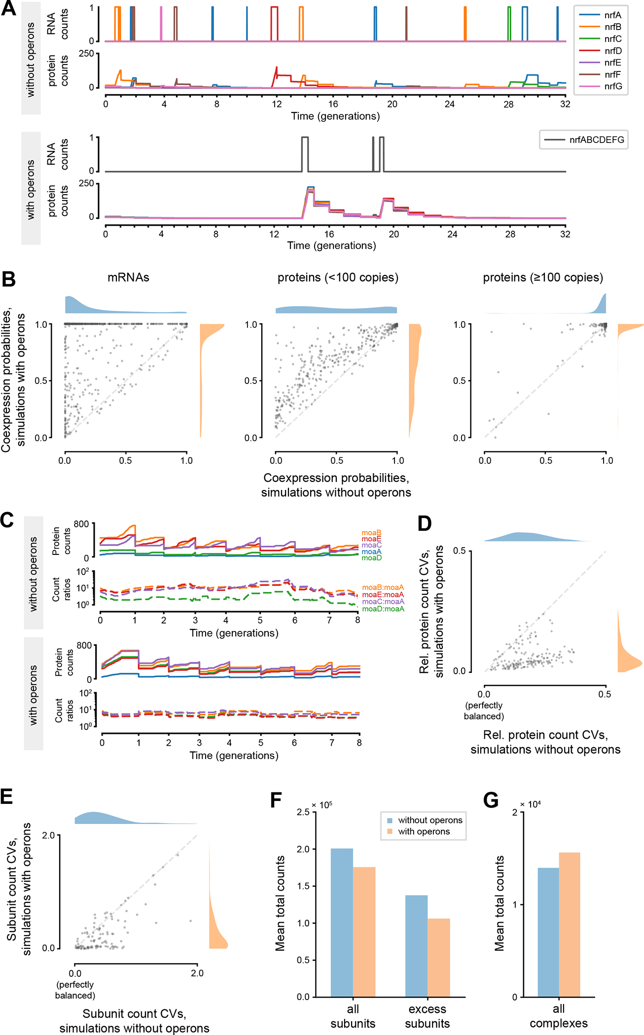
Comparisons between simulations with and without operons suggested possible benefits operons can bring to bacteria. (A) Simulated dynamics of mRNA and protein counts for genes in the nrfABCDEFG operon, in simulations without and with operons. (B) Comparisons of coexpression probabilities of each operon, between simulations with and without operons. Operons increase these probabilities at the mRNA level (left) and, for low-expression genes, at the protein level (middle), but not for high-expression genes at the protein level (right). See Table S3 for full data. (C) Simulated dynamics of absolute and relative protein counts for genes in the moaABDEC operon, in simulations without and with operons. (D) Comparison of coefficients of variation (CV) calculated from relative protein counts for each operon, between simulations with and without operons. See Table S4 for full data. (E) Comparison of coefficients of variation calculated from subunit counts normalized with complexation stoichiometries for each protein complex, between simulations with and without operons. See Table S5 for full data. (F) Comparison of total counts of all protein subunits and excess subunits between simulations with and without operons. (G) Comparison of total counts of all protein complexes between simulations with and without operons. In all panes, the reported values are averages of the respective values taken from each simulated cell with a fully completed cell cycle (n=768 for simulations without operons, n=758 for simulations with operons).

To further explore this hypothesis – that operons may be necessary to synchronize the expression of functionally dependent, low-expression genes – in a broader scope, for each polycistronic operon we added to the whole-cell model, we calculated the “co-expression probability” of its constituent genes, and compared these probabilities between simulations that were run with operons and without operons (STAR Methods). We defined the co-expression probability as the length of simulated time when the products (either mRNA or protein) of all genes within the group have nonzero counts, divided by the length of simulated time when at least one of the gene products have nonzero counts. We chose to divide by the length of time when at least one of the products exist, rather than the total simulation time, to normalize against the widely different overall expression frequencies of different operons. 32 operons that have one or more constituent genes that were never expressed in simulations without operons were excluded from this analysis. When these co-expression probabilities were calculated at the level of mRNAs, the updated simulations with operons had most of the probabilities clustered around 1, whereas the old simulations had most probabilities clustered around 0, reflecting a substantial increase in these probabilities as a result of using operons (Figure 5B, left). In total, the mRNA co-expression probability increased for 710 (94%) operons among 756 polycistronic operons with nonzero expression, with 392 (52%) operons seeing a probability boost by more than 10-fold.

When we calculated the co-expression probabilities using protein counts, however, the story diverged between operons with low expression and high expression. We divided the 756 operons into two similarly sized groups based on the averaged protein copy numbers expressed from the genes constituting each operon in simulations run without operon structures. Low-expression operons were defined as operons whose average protein copy numbers were lower than 100, while high-expression operons were defined as operons with protein copy numbers higher than 100. For low-expression operons (359 operons), the addition of operons still resulted in an increase in co-expression probabilities, with 307 (86%) of the gene groups seeing an increased probability in simulations with operons (Figure 5B, middle). For high-expression operons (397 operons), the increase in co-expression probabilities was less pronounced, mainly because most of the gene groups already had probabilities that were close to 1 in simulations without operons (Figure 5B, right). Since proteins are more stable than mRNAs by many orders of magnitude, many proteins remain in existence long after their respective mRNAs have degraded, which makes it more likely for a group of proteins to simultaneously have nonzero counts, even with uncoordinated expression at the mRNA level. These results suggested that we would need a different hypothesis to explain the utility of operons for these high-expression genes. Table S3 lists the calculated co-expression probabilities of all 756 operons in both sets of simulations.

Relative quantities of proteins expressed from the same operon were under tighter control in the updated model

Growing evidence suggests that many components of the bacterial transcription and translation machinery have evolved to maintain a specific stoichiometry between certain groups of functionally related proteins²². The relative abundance of enzymes in many metabolic pathways, for instance, were observed to be similar between E. coli and B. subtilis, despite these two species being separated by two billion years of divergent evolution³². While it is still unclear why a tight control of protein stoichiometries is necessary for many of these functional gene groups, some have hypothesized that operons may help bacterial cells enforce a tighter control over these stoichiometries¹⁹. Since stochastic fluctuations in protein copy numbers mostly originate from transcriptional noise^7,51, expressing multiple genes as part of the same transcript would eliminate a major source of noise that could affect the relative abundance of their protein products.

To explore this idea in the whole-cell model, we first focused on the moaABDEC operon, whose constituent genes encode for enzymes that are part of the molybdopterin biosynthesis pathway in E. coli⁵². Four enzymes (MoaA, MoaC, MoaD, and MoaE) that are encoded by genes in this operon have conserved relative abundances between E. coli and B. subtilis³², suggesting that maintaining the stoichiometry between these proteins is important for the functionality of the metabolic pathway. In simulations without operons, the relative copy numbers of the proteins produced from these genes fluctuated, with ratios changing up to 13.0-fold throughout 8 generations of simulated cell growth (Figure 5C). In simulations with operons, however, despite the dynamic changes in the absolute copy numbers of each protein, the relative copy numbers remained relatively stable, with ratios only changing up to 2.2-fold throughout the same number of simulated generations (Figure 5D). In both sets of simulations, all five proteins were present at all simulated timepoints, indicating that the addition of operons would have had minimal effects on the co-expression probabilities of this operon.

We performed a similar analysis for 173 high-expression operons whose protein products were constantly present through all timepoints in both sets of simulations. We first normalized each protein’s copy numbers at each timestep by its mean protein copy number through all timesteps of the simulation. Then, for each operon, we calculated the coefficient of variation (CV, standard deviation divided by the mean) between the normalized copy numbers of the constituent proteins at each timestep. These coefficients quantify how far the expression stoichiometries between the proteins in the operon have deviated from their time-averaged expression stoichiometries. If the expression stoichiometries are perfectly constant throughout the entire simulation, the coefficients should be equal to zero at every timestep, but any deviance from the average would lead to higher coefficients. When we plot the time-averaged value of the coefficient of variation for each operon in simulations with operons versus simulations without operons, the value is lower in simulations with operons for 159 (92%) of the operons (Figure 5D), suggesting that operons help maintain more stable stoichiometries for these groups of proteins. Table S4 lists the calculated coefficients of variation of all 173 operons in both sets of simulations.

The addition of operons helped the model produce protein complex subunits in quantities closer to their known complexation stoichiometries

E. coli has been shown to express the protein subunits of heteromeric protein complexes in quantities that are proportional to the stoichiometries of the subunits in the protein complex⁵³. In this case, the benefits of stoichiometric expression are more obvious – producing excess numbers of subunits is both a waste of cellular resources, and a potential hazard, as these excess subunits can form protein aggregates that can adversely affect the cell^54–57. Thus, it is not surprising that genes encoding for protein subunits of heteromeric complexes are often found on the same operon^53,58. Among the 1,093 protein complexes that we incorporated into this version of the whole-cell model, 271 complexes were heteromeric, and 173 heteromeric complexes had all of its constituent subunits expressed from the same operon. We hypothesized that for these 173 complexes, adding operons to the simulations would not only make the expression stoichiometries of the subunits more stable through time, but also more consistent on average with the known complexation stoichiometries of the protein complex.

Among these 173 protein complexes, we selected 107 complexes whose exact subunit stoichiometries were known according to EcoCyc, and whose subunits were not shared with other protein complexes. For each of these complexes, we calculated the time-averaged copy numbers of each subunit (including those that are already part of the protein complex), in simulations run with operons and without operons. We then normalized each subunit’s counts with their stoichiometries within the complex, and calculated the coefficient of variation between these normalized subunit counts for each protein complex. This coefficient, similarly, measures how far the averaged relative quantities of subunits deviates from their known stoichiometries within the complex, and would be equal to zero if the average expression stoichiometries of the subunits perfectly match the complexation stoichiometries. When these coefficients were compared between the two sets of simulations, we observed that their values decreased in the simulations with operons for 85 (79%) complexes (Figure 5E). Table S5 lists the calculated coefficients of variation of all 107 protein complexes in both sets of simulations.

We also quantified how the addition of operons affects the total copy numbers of excess subunits and protein complexes in the model. When we compared the mean total counts of protein subunits that constitute the 107 complexes, the simulations with operons expressed 13% fewer subunits overall compared to the simulations without operons, and 23% fewer excess subunits that were not incorporated into the complexes (Figure 5F). Despite having less subunits to work with, the mean total copy numbers of the 107 full complexes increased by 12% in simulations with operons (Figure 5G), demonstrating the improved efficiency in which the simulations with operons express and build these protein complexes.

Discussion

In this work, we built an updated version of the E. coli whole-cell model that accounts for the known operon structures of the E. coli genome and used the simulated E. coli cells to explore how these operon structures can benefit bacteria. In the process of integrating heterogeneous data into the model, we identified conflicts between the input data that resulted from computational artifacts, curation errors, or simple experimental errors, which we iteratively resolved through deep curation using the simulation outputs. The two versions of the model – one with 788 polycistronic operons, and one where every gene is its own transcription unit – were each used to simulate a group of cells and were compared in terms of their gene expression dynamics, making use of the unique abilities of the whole-cell model in performing large-scale in silico experiments where every single molecule can be precisely quantified.

Most bacteria, including E. coli, must work to overcome challenges that come from their smaller cell sizes, as compared to eukaryotes. One such challenge is that individual E. coli cells do not have enough gene expression capacity to express all genes that may be necessary for survival under rapidly changing environments^14,59,60. This problem is exacerbated by the fact that adapting to survive in a changing environment, such as metabolizing newly introduced nutrients or countering antibiotics, often requires the simultaneous expression of multiple genes. Our modeling results predict that co-regulating these genes through operons can increase the likelihood that the genes are co-expressed at a genome-wide level, especially for low-expression genes that only a small subset of cells within a colony is likely to express at any given time. This would allow a colony of E. coli cells to keep the expression levels of these genes at a low level, and thus minimize the use of cellular resources on these genes, while maintaining a high probability that one or more cells would simultaneously express all of the genes required for a specific environment. In this sense, operons allow bacteria to be more efficient with their bet-hedging strategies⁶¹ by expressing more genes that are only functionally relevant in rare circumstances, while minimizing the metabolic cost associated with the expression of these genes under normal circumstances. Combined with recent efforts to represent multi-cell colonies and mechanisms of antibiotic resistance with the E. coli whole-cell model⁶², we may be able to use the model to explore these strategies in greater detail in future projects.

Another size-imposed challenge for bacteria is that the quantities of important gene products within the cell are subject to stochastic fluctuations^59,63. Our modeling results predict that some operons in E. coli serve the function of dampening the impacts of these fluctuations by stabilizing the stoichiometry of mRNA expression between functionally related genes, as previous studies have demonstrated on a smaller scale^18,19. While the transcription of mRNAs from these operons are still noisy, the fixed stoichiometries between individual genes help decrease excess expression of unused products, and also ensure that stochastic dips in the expression of a single gene do not bottleneck the other genes that serve the same function. This functionality of operons is important when the gene products of the operon form complexes with fixed stoichiometries, and, with growing evidence, when the products do not form a physical complex as well^22,32. While this work only considered the mRNA operons of E. coli, the structures of the rRNA operons of E. coli also illustrate this functionality. 6 of the 7 rRNA operons of E. coli transcribe RNAs that contain one copy of each rRNA species (5S, 16S, and 23S rRNA; the rrnD operon is the only exception with an extra copy of 5S rRNA)^64–66, that are later complexed into a ribosome in a 1:1:1 ratio. Co-expressing these three genes as a single transcription unit would ensure that the three rRNA species are always transcribed in the same ratio, such that no excess rRNA species are produced, and the complexation of ribosomes is not bottlenecked by a single rRNA species.

As suggested in the introduction, more targeted experimental studies would be necessary to validate these predictions made by our model on the utility of operons. For example, the model predicts the existence of many low-expression operons where operons serve the role of increasing the coexpression probabilities of its constituent genes. Many of these operons consist of genes that need to be coexpressed for the E. coli cell to adapt to a specific environment, such as a newly introduced carbon source. An engineered strain of E. coli, where the constituent genes of such an operon are decoupled to be expressed from separate promoters, would be expected to have a lower coexpression probability for these genes, and thus have reduced colony-level fitness in shifting environments specific to the decoupled operon compared to wildtype cells. Reporter genes could be used to experimentally measure coexpression probabilities, while overall fitness could be quantified through changes in growth rates. The results presented in this work may help in the selection of the most appropriate operons for such experimental studies.

In the process of updating the whole-cell model to transcribe polycistronic transcripts, we uncovered computational artifacts in conventional RNA-Seq alignment algorithms that may lead these algorithms to falsely report the read counts of the shortest genes as zero. We demonstrated that we can calculate more accurate read counts for these short genes by accounting for the known transcription unit structures of the genomes that these RNAs were transcribed from. To our knowledge, none of the currently available RNA-Seq alignment algorithms for bacterial RNA make use of information regarding the transcription unit structures of bacterial genomes. In contrast, there are various RNA-Seq alignment algorithms developed for eukaryotic RNA which make use of the known data on the intron-exon boundaries of the species that the RNA sample was taken from, in order to improve the accuracy of read counts and to quantify splicing isoforms^67,68. For bacterial species like E. coli whose transcription unit structures are well-characterized, utilizing these known structures during the alignment, similar to how these eukaryotic RNA alignment algorithms utilize intron-exon structures, could potentially help avoid these issues with short genes and improve the general accuracy of read count calculations.

While this work takes a step forward in bringing the E. coli whole-cell model closer to the actual biology of E. coli cells, the model still falls short of fully representing our ever-evolving knowledge of E. coli’s transcription unit structures. Many operon-specific regulatory mechanisms, some of which may be relevant to the utility of operons under certain contexts, were not incorporated into this version of the whole-cell model. For instance, it has been shown that different mRNA isoforms can have distinct secondary structures that impact translation, which can lead to the same gene having different translation efficiencies depending on which mRNA isoform it was translated from^69,70, whereas our model currently assumes a constant translation efficiency for each gene. Translational coupling, where the translation of genes on the same transcript become interdependent, has been observed to occur in many E. coli operons^71–73, which would further reduce the stochastic variations in protein stoichiometries for these operons. Lastly, it has been suggested that the translation efficiency of genes can be 6 times higher for transcripts that are undergoing transcription, compared to transcripts that have been fully transcribed⁷⁴, which would shift the relative expression levels of proteins that are produced from longer operons, as genes that are closer to the start of the operon will have more time to be translated while the mRNA is being transcribed.

We would also like to emphasize that our results do not invalidate the other hypotheses that have been proposed on the utility of operons. In fact, it is likely that all of the proposed mechanisms contribute in concert to maintain the existence of operons in bacterial genomes. Some of the E. coli operons that we have analyzed in this study neither improved the co-expression probabilities of their constituent genes, nor stabilized the stoichiometric balance of their proteins, suggesting that other theories may better explain the existence of these operons, assuming that our model’s parameters and assumptions for the operon were largely correct. A targeted probe into these operons may lead to interesting discoveries about their functional roles or point to errors in our current understanding of these operons.

In sum, our work presents the expansion of the E. coli whole-cell model to account for transcription unit structures of the E. coli genome, and the biological insights that can be gained from both the process of expanding and the simulations arising from the expanded model. While this work utilized data generated from many recently developed RNA sequencing techniques, it also highlighted limitations in our current technologies and knowledge, particularly with regards to the accurate, quantitative characterization of longer, polycistronic RNA molecules. Further advancements in long-read sequencing technologies would allow us to use more direct and accurate measurements to parameterize the transcription and degradation of polycistronic transcription units, instead of resorting to indirectly estimated parameters as we have done in this work. We also hope that this expansion lays a foundation for more data and mechanisms to be added to the whole-cell model in the future, including the structures and processing of rRNA and tRNA operons, the aforementioned operon-specific regulatory mechanisms, and more detailed representations of the components of the E. coli chromosome. These updates, in combination with the other avenues of expansion that are ongoing within the E. coli Whole-cell Modeling Project^12,17,75, will bring the whole-cell model closer to a complete digital replica of E. coli cells that can provide us with even deeper and more comprehensive biological insights.

STAR Methods

RESOURCE AVAILABILITY

Lead Contact

Further information and requests for resources should be directed to and will be fulfilled by the lead contact, Markus Covert (mcovert@stanford.edu).

Materials availability

This study did not generate new unique reagents.

Data and code availability

• All data reported in this paper will be shared by the lead contact upon request.

• All code for the E. coli whole-cell model, Rend-seq data analysis, and the manual alignment of short genes have been made available in GitHub repositories with DOIs (See key resources table for links). Descriptions of the simulations and analyses performed with the whole-cell model can be found in this paper’s quantification and statistical analysis section.

• Any additional information required to reanalyze the data reported in this paper is available from the lead contact upon request.

METHOD DETAILS

Whole-cell modeling concepts

Whole-cell models are mathematical representations of cells that cover all of the known biological functions of their genes and molecular components¹². As mentioned in the introduction, a whole-cell model is composed of multiple submodels that each represent a particular biological process within the cell that uses a mathematical framework that is most appropriate for the given process. The choice of the mathematical framework depends on the dynamic properties of the cellular function in question, as well as the scope of the available knowledge and data we have for the specific function. For instance, in the E. coli whole-cell model, metabolism is represented with a modified flux balance analysis (FBA) model⁷⁷, while transcription and translation are represented with a stochastic model. These submodels are linked together into the whole-cell model under the assumption that each of the submodels are functionally independent from each other over short time intervals. The whole-cell model runs in discrete timesteps which by default are set to be 1 second long. At the start of each timestep, each submodel takes in the current state of the simulated cell as input, and calculates the updates that need to happen to the state of the cell during the given timestep. At the end of each timestep, the updates submitted by each submodel are integrated to yield the next state of the cell. This process is repeated until the cell reaches its cell division criteria and divides into two daughter cells. This modular framework was the key to our success in building a unified model of an entire cell that utilizes tens of thousands of heterogeneous parameters.

More information about the different submodels for each of the biological processes within the E. coli whole-cell model are provided in great detail in previous publications^12,14. Here, we will primarily focus on describing the transcription submodel, as this submodel is most relevant to the updates to the model presented by this work.

Transcription submodel of the E. coli whole-cell model

The transcription submodel within the E. coli whole-cell model is responsible for initiating the transcription of RNAs and elongating RNAs that are being transcribed¹⁴. At the beginning of each simulation timestep, the transcription submodel reads the counts of free RNA polymerases $(\left.N_{\mathrm{R}\mathrm{N}\mathrm{A}\mathrm{P},f}\right)$ from the simulation state, and determines how many RNA polymerases would be allocated to each transcription unit $\left(n_{\text{init},i}\right)$ for transcription initiation by sampling from a multinomial distribution.

$$n_{\text{init},i}=\mathrm{m}\mathrm{u}\mathrm{l}\mathrm{t}\mathrm{i}\mathrm{n}\mathrm{o}\mathrm{m}\mathrm{i}\mathrm{a}\mathrm{l}\left(p_{act,\mathrm{R}\mathrm{N}\mathrm{A}\mathrm{P}}\cdot N_{\mathrm{R}\mathrm{N}\mathrm{A}\mathrm{P},f},p_{\text{synth},i}\right)$$

Here, $p_{act,\mathrm{R}\mathrm{N}\mathrm{A}\mathrm{P}}$ is the RNA polymerase activation probability, which is derived from the experimentally measured fraction of active RNA polymerases in E. coli cells³⁰. $p_{\text{synth,}i}$ is the synthesis probability that is specific to each transcription unit, which determines how frequently each transcription unit will be transcribed. This probability, in turn, is calculated by first assuming that the concentration of each RNA species is at steady state:

$$\frac{d{m}_i}{dt}=v_{\text{synth},i}-m_i\cdot (\frac{\mathrm{l}\mathrm{n}2}{\tau }+\frac{\mathrm{l}\mathrm{n}2}{t_{1/2,i}})=0$$

$$v_{\text{synth},i}=m_i\cdot (\frac{\mathrm{l}\mathrm{n}2}{\tau }+\frac{\mathrm{l}\mathrm{n}2}{t_{1/2,i}})$$

Here, $m_i$ is the concentration of RNA $i$, $\tau$ is the doubling time of the cell, and $t_{1/2,i}$ is the degradation half-life of RNA $i$. The concentration $m_i$ for each mRNA species can be calculated from the measured total mass of all mRNAs^29,30 and the RNA-Seq read counts of each mRNA species¹⁴. Thus, $v_{\text{synth},i}$ is the synthesis rate for RNA $i$ that is required for the RNA’s concentration to remain at steady state, given the RNA-Seq read counts and the degradation half-life of the RNA. $p_{\text{synth},i}$ is calculated by normalizing the values of $v_{\text{synth}}$ for each transcript by the sum of $v_{\text{synth}}$ values of all transcripts:

$$p_{\text{synth},i}=\frac{v_{\text{synth},i}}{\sum _j{v}_{\text{synth},j}}$$

In sum, to calculate $p_{\text{synth,}i}$, which determines how frequently an RNA species will be transcribed, we first need to know the RNA-Seq read counts (or equivalently, relative RNA copy numbers) and the degradation half-life of the RNA species. Thus, to parameterize a transcription submodel that can transcribe polycistronic mRNAs, we first needed to estimate the values of these two parameters for polycistronic mRNAs.

Integration of heterogeneous data and deep curation

The E. coli whole-cell model integrates more than 19,000 experimentally measured parameters from hundreds of heterogeneous sources into a unified model of an entire cell¹⁴. Because of the inherently noisy nature of biological data, and the different experimental conditions that each set of parameters was measured from, we often encountered cases where the datasets that we collected were not cross-consistent when we attempted to put them together into the whole-cell model. These inconsistencies usually manifested themselves as errors in our parameter calculation step, or unstable simulations that were unable to double the mass of all of its components consistently through multiple cell cycles. How we identify and resolve these discrepancies – the process we named “deep curation” – was the theme of many of our previous publications that use the E. coli whole-cell model^14,17,75.

Our general approach of resolving these discrepancies involves a fitting process where we attempt to find a set of parameters that is cross-consistent while not allowing the parameters to deviate too far from their original experimentally measured values. We determine how far each parameter would be allowed to deviate from its original value based on how much error we expect the measured value to hold. In some sense, this could be viewed as a coarse Bayesian approach to reconciling inconsistent datasets, where we use the prior distributions of the two datasets to find a set of maximum-likelihood parameters under the constraint that they need to be cross-consistent with each other. Unfortunately, for most biological data, we only have a qualitative sense of how large the errors for each data point would be, and thus are often forced to make assumptions about the relative accuracies (and thus, the prior distributions) of different datasets in this fitting process. In some cases, if the discrepancies are big enough, and alternative experimental measurements that support the corrections exist, we can further verify the corrections that we made to these parameters with these alternative measurements, and suggest model-guided corrections to these parameters with higher confidence.

In this work, the major inconsistency between data points that we needed to address was the conflict between the newly integrated transcription unit structures and the gene-level RNA-Seq read counts that the model was already using. We addressed this inconsistency initially by using NNLS to find a set of parameters that are both (i) consistent with the transcription unit structures and (ii) as consistent as possible with the RNA-Seq read counts, based on the knowledge that RNA-Seq read counts often contain large errors, especially for genes with low expression levels. As we considered making corrections to the two datasets for more cross-consistency, we needed to be wary of overfitting, since transcription unit structures can always be adjusted (e.g. by having each gene be transcribed as their own single-gene transcription unit, in the extreme case) to be perfectly consistent to an arbitrary array of RNA-Seq read counts. To minimize overfitting, we chose to make the model-guided corrections to either the transcription unit structures or the RNA-Seq read counts to resolve these discrepancies if and only if when the discrepancies between these two datasets were substantial enough, and there existed alternative datasets that can be used to verify our corrections, as in the case for the operons highlighted in Figure 2 and Figure 3A.

Nonnegative least squares for relative RNA counts

As described in the main text, to estimate relative RNA copy numbers at the level of individual transcripts, we formulated a linear system of equations under the assumption that a gene’s RNA-Seq read count must be similar to the summed copy numbers of all transcription units that covers the gene (Figure 2A). We started from the RegulonDB/EcoCyc-curated list of mRNA operons and their transcription units, and constructed a binary matrix $S$ of size 4,527 × 3,182 for each operon that maps each transcript to its constituent genes, where $S_{ij}=1$ if gene $j$ belongs to transcript $i$, and $S_{ij}=0$ if not. For the 3-gene cynTSX operon, for example, RegulonDB/EcoCyc lists two transcription units cynTSX and cynTS (Figure 2A, top), which translates to a 3×2 matrix $S$. In the ideal case, this matrix multiplied with the vector of transcript-level counts should yield the vector of gene-level read counts (Figure 2A, middle). Because of inherent errors in both the transcription unit structures in matrix $S$ and the vector of gene-level read counts, however, we could not find exact solutions to these equations for many operons and had to resort to finding optimal approximate solutions using least squares methods. Since RNA counts cannot be negative, we used a nonnegative least squares (NNLS) algorithm⁷⁸ that imposes a nonnegative constraint to the solution of the canonical least squares problem to solve these equations (Figure 2A, bottom). Since most of the elements (99.96%) in matrix $S$ had a value of zero, the matrix was stored using scipy‘s compressed sparse row matrix format. The transcript-level RNA copy numbers, $x$, can be estimated from matrix $S$ and the vector of gene-level RNA-Seq read counts ($b$) by solving the following non-negative least squares (NNLS) problem:

$$x={\mathrm{a}\mathrm{r}\mathrm{g}\mathrm{m}\mathrm{i}\mathrm{n}}_{x\ge 0}{\parallel Sx-b\parallel }^2$$

To solve the NNLS problem, a custom Python function was built (wholecell/utils/fast_nonnegative_least_squares.py) that utilizes the unique structural properties of matrix 𝑆. Since matrix 𝑆 is a sparse matrix that can be decomposed into orthogonal submatrices that each represent the transcription unit structures of a single operon, the function first splits the problem into smaller NNLS problems, which are then solved individually using the built-in nnls function of the scipy package⁷⁸. The solutions to these subproblems are then concatenated to return the full solution $x$. This optimized function was more than 10 times faster than naïvely using the nnls function for the full matrix and was critical in keeping the runtime of the updated simulations comparable to the original simulations. The final normalized transcript-level RNA counts that we calculated for each mRNA transcript can be found in file runscripts/operon_paper/mRNA_transcript_table.tsv.

It is worth noting that while the solution 𝑥 returned by the NNLS algorithm is guaranteed to be optimal, there may exist multiple alternative solutions that have the same value of $\parallel Sx-b{\parallel }^2$. Thus, for an arbitrary operon, we cannot claim that the transcript-level RNA-Seq read counts that we estimated using NNLS are uniquely accurate. The calculated read counts are one of many sets of parameters that are most consistent with the gene-level read counts while complying with the constraints given by the transcription unit structures, and the confirmation of exact transcript-level read counts would likely require experiments that directly target the transcription units in question. For the purposes of this work, however, the existence of alternative solutions did not affect the conclusions drawn from the later sections of this work, as the guarantee of optimality was sufficient for us to identify the discrepancies between gene-level RNA-Seq read counts and transcription unit structures for particular operons.

Nonnegative least squares for degradation rate constants

To estimate degradation rate constants at the level of individual transcripts, we assumed that the observed gene-level degradation rate constant for a certain gene should be equal to the abundance-weighted sum of degradation rate constants of all transcription units that contain the given gene. More specifically, if the measured degradation rate constant for a gene is $k_{\mathrm{d}\mathrm{e}\mathrm{g}}$, and the gene is transcribed as part of transcription units A and B, whose degradation rate constants are $k_A$ and $k_B$, and whose concentrations are [$A$] and [$B$], respectively, the following equation must hold between these constants.

$$\frac{d[G]}{dt}=-k_{\mathrm{d}\mathrm{e}\mathrm{g}}[G]=-k_A[A]-k_B[B]$$

$$k_{\mathrm{d}\mathrm{e}\mathrm{g}}=k_A\frac{[A]}{[G]}+k_B\frac{[B]}{[G]}$$

Here, [$G$] is the total concentration of the given gene, which is equal to $[A]+[B$]. Thus, the values $[A]/[G]$ and $[B]/[G]$ are equal to the normalized abundances of the transcription units that cover the given gene. From this linear relationship, we could construct a similar system of equations for each operon, but instead of the transcription unit-gene matrix $S$, we constructed the relative abundance matrix $R$, whose elements represent the ratios $[A]/[G]$ and $[B]/[G]$ in the equation above. More specifically, the value of $R_{ij}$ is equal to the normalized counts of transcription unit $j$, among all transcription units that cover gene $i$. The relative counts of each transcription unit were taken from the earlier solution of the NNLS problem for relative RNA counts. Under ideal circumstances, this matrix $R$, when multiplied with the vector of transcript-level degradation rate constants $x$, would yield the vector of measured gene-level degradation rate constants $k$ (Figure S1). Again, a feasible solution did not exist for many operons, so we used the NNLS algorithm to solve the following optimization problem:

$$x={\mathrm{a}\mathrm{r}\mathrm{g}\mathrm{m}\mathrm{i}\mathrm{n}}_{x\ge 0}{\parallel Rx-k\parallel }^2$$

For a small number of operons, however, we did have experimentally measured values for the degradation half-lives of polycistronic transcripts within the operon²⁸. For these transcription units, we chose to not only use these measured values for their degradation rates, but also use these values to further constrain the optimization problem for other unmeasured degradation rate constants within the operon. From the original matrix $R$, we built a submatrix consisting of columns that represent transcription units whose degradation rate constants were experimentally measured $\left(R_m\right)$ and a submatrix for transcription units without experimental measurements $\left(R_{-m}\right)$. This allowed us to solve the following optimization problem, which is constrained by both the gene-level degradation rate constants ($k$) and the measured transcript-level degradation rate constants $\left(x_m\right)$, to estimate the unknown degradation rate constants $\left(x_{-m}\right)$:

$$x_{-m}={\mathrm{a}\mathrm{r}\mathrm{g}\mathrm{m}\mathrm{i}\mathrm{n}}_{x\ge 0}{∥R_{-m}x+R_m{x}_m-k∥}^2$$

Lastly, unlike relative RNA counts, degradation rate constants must have nonzero values. To prevent the optimization problem from returning degradation rate constants of zero, we added another constraint to the optimization problem that requires all degradation rate constants to be equal to or greater than the smallest mRNA degradation rate constant that has been measured experimentally at the gene level^23,28. Since the nnls function of scipy did not support arbitrary lower bounds for the solution other than zero, we solved the following NNLS problem that is mathematically equivalent to an optimization problem with a nonzero lower bound for the solution:

$$x_{-m}={\mathrm{a}\mathrm{r}\mathrm{g}\mathrm{m}\mathrm{i}\mathrm{n}}_{x\ge 0}{∥R_{-m}x+R_m{x}_m+R_{-m}{k}_{\text{min}}-k∥}^2+k_{\text{min}}$$

Here, $k_{\mathrm{m}\mathrm{i}\mathrm{n}}$ is a vector of the same length as $x_{-m}$ that is fully populated with the minimum value of the degradation rate constant, which ensures that every element of $x_{-m}$ is greater than or equal to this minimum value. We used the same custom Python function built for relative RNA counts to solve this optimization problem more efficiently. The final transcript-level degradation rate constants that we calculated for each mRNA transcript can be found in file runscripts/operon_paper/mRNA_transcript_table.tsv.

As in the case for transcript-level RNA-Seq counts, the solution $x$ returned by the NNLS algorithm is guaranteed to be optimal; however, there may exist multiple alternative solutions that are just as optimal. The confirmation of exact transcript-level degradation rate constants would require experiments that directly target the transcription units, as demonstrated by previous works²⁸.

Updates to the E. coli whole-cell model: parameter calculator

The parameter calculator (ParCa) is a module of the E. coli whole-cell model that is responsible for converting raw experimental parameters into actual simulation parameters that the model directly uses to simulate E. coli cells¹². Several updates were made to the ParCa to support the transcription of polycistronic transcripts, with the most important updates listed here.

First, a new data file (See repository for the E. coli whole-cell model, file reconstruction/ecoli/flat/transcription_units.tsv) was added to the collection of raw data that is given as an input to the ParCa. This file, built from data that is available through EcoCyc version 26.0²⁷, contains a curated table of all transcription units that have been identified in the E. coli genome, along with their IDs, common names, constituent genes, left and right end positions on the genome, transcription directions, and associated evidence codes. When run with the option operons_on=True, the ParCa now uses the list of transcription units in this file to build its list of RNAs and their sequences. When run with the option operons_on=False, the ParCa retains its old behavior where it uses the list of genes in the file reconstruction/ecoli/flat/genes.tsv to build its list of RNAs. This option in the ParCa allowed us to easily switch back and forth between the two versions of the model without making any changes to the simulation itself. Any transcription units listed on EcoCyc that are not fully composed of mRNA-encoding genes were manually excluded from the file for this version of the model.

One of the core functions of the ParCa is to adjust the expression levels of mRNA genes that encode for subunits of RNA polymerases and ribosomes, such that the simulated cell can produce enough of these enzymes to double its mass within its expected doubling time¹⁴. To fit these parameters, the ParCa first calculates the amount of RNA polymerases and ribosomes that would be needed to double the cell’s mass within the given doubling time, and traces them back to the expression levels for these genes that would be needed to produce the calculated amounts of RNA polymerases and ribosomes. Since these subunits are now transcribed as part of polycistronic operons, however, additional steps were needed to convert the counts of proteins to the required expression levels of the transcription units. More specifically, in the fitExpression function of the main ParCa script (reconstruction/ecoli/fit_sim_data_1.py), where the expression levels of individual RNAs are set to match the expected protein levels, the NNLS function is now used to compute the synthesis probabilities of transcription units that most accurately approximate the hypothetical expression levels of each gene that matches the protein levels. This was repeated for each iteration of the fitting process, at which the required counts of RNA polymerase/ribosomal subunits to double the mass were recalculated using the most recently calculated expression levels of RNAs. This update allowed the ParCa to fit the expression levels of these genes while adhering to the stoichiometric restrictions provided by the transcription unit structures of the operons that these genes belong to.

Updates to the E. coli whole-cell model: transcription submodel

The biggest update to the transcription submodel was the restructuring of the input data that the transcription submodel uses to initialize transcription events. In the original version of the model, the transcription submodel used data from a single table of monocistronic RNAs, which contained all necessary information to model the transcription of these RNAs including transcript lengths, RNA types (mRNA, tRNA, etc.), genomic coordinates etc. In the updated version, the transcription submodel now uses two distinct tables that each contain necessary data for “cistrons” and “RNAs”, respectively. Cistrons are the individual stretches on RNA transcripts that encode for a single gene, and are represented by the ID of the corresponding gene followed by a suffix (e.g. EG10001_RNA). RNAs are the physical RNA transcript molecules that can be either monocistronic or polycistronic, and are represented by either the ID of the transcription unit listed in the newly added transcription units data file followed by a compartment tag (e.g. TU-8381[c]) or, in the case of monocistronic RNAs whose encoding gene was not covered by any of the transcription units in the transcription units file, the ID of the corresponding cistron followed by a compartment tag (e.g. EG10001_RNA[c]). The updated RNA table takes on the role of the old table of monocistronic RNAs, by providing the transcription submodel with the information necessary to transcribe RNA molecules. The cistron table serves as a reference point whenever there is a need to map the properties of transcription units to the properties of individual genes.

Updates to the E. coli whole-cell model: translation submodel

The translation submodel of the E. coli whole-cell model is responsible for initializing translation by assigning ribosomes to mRNAs and elongating the polypeptides that are synthesized from these active ribosomes¹⁴. In the original version of the model, because all mRNAs were monocistronic, each mRNA was associated with a single polypeptide, which greatly simplified the process of assigning ribosomes to mRNAs based on the translation efficiencies⁵³ of each gene. In the updated model, the assignment of ribosomes that need to be initiated for each protein monomer happens through multiple steps. First, the translation submodel calculates the total copy numbers of each translatable mRNA gene, using the counts of both fully transcribed and nascent mRNA molecules. Note that for a gene within a nascent mRNA to be translatable, the mRNA needs to be transcribed long enough so that the ribosome binding site for the gene exists for the mRNA molecule. For simplicity, our model assumes that a gene is translatable if the first base of its coding sequence has been transcribed. Next, ribosomes are distributed to each gene using a multinomial distribution, where the translation probability of each gene is proportional to their translation efficiency multiplied by their total mRNA copy number. These ribosomes are then positioned to appropriate locations on each transcript, based on the relative position of the gene within the transcription unit. Thus, many ribosomes can now have nonzero starting locations on the transcript, if they are translating genes that are not the first gene on a particular mRNA transcript.

Updates to the E. coli whole-cell model: comparison analysis

In order to facilitate comparisons between simulations with and without operons, a new class of “comparison” analysis scripts was added to the whole-cell model. This analysis class is similar to the pre-existing variant analysis class, which compares simulation outputs between variant simulations that are run under a set of simulation parameters that are only slightly different from each other, and originate from the same ParCa run¹². The comparison analysis class, on the other hand, allows for the comparison of two sets of simulations that were run with two entirely different sets of simulation parameters that originate from two different runs of the ParCa. Since the updated version of the model with operons requires a different option for the ParCa, this new class of analysis was needed to compare the outputs between the original and updated versions of the model. Examples of newly added analysis scripts that fall into this category are presented in the quantification and statistical analysis section.

Rend-seq data analysis

Rend-seq read counts data were taken directly from the Gene Expression Omnibus dataset (GSE95211, See Key Resources Table) provided by the original publication that developed this method³². Custom Python scripts were used to plot the read counts and overlay the data with the known locations of genes on the E. coli reference genome (U00096.2). All scripts that were used for this purpose were made available through a separate public GitHub repository (See Key Resources Table for link). Within this repository, the file runscripts/paper_figures.sh contains the specific commands that were used to generate the Rend-seq figures presented in this paper.

It is worth noting here that while the primary purpose of Rend sequencing is to identify the 5’ and 3’-ends of RNAs, Rend-seq data can also be used to quantify the relative expression levels of different genes along the same operon, as demonstrated by the publication from which the data was sourced³². In this work, we chose to use the Rend-seq data only for the purpose of verifying potential 5’ and 3’-ends suggested by the model, and not for quantifying gene-level expression levels, mainly because the sequencing depth of the Rend-seq dataset was not sufficient to provide expression levels for many of the low-expression operons of E. coli. In the Rend-seq dataset, many low-expression operons did not have a sufficient amount of aligned reads for their relative expression levels to be evaluated accurately. For the purposes of parameterizing a whole-cell model, we needed to use the data from more traditional RNA-Seq, which provided us with sufficient sequencing depth and thus more accurate RNA read counts for all E. coli genes.

Manual alignment of RNA reads to short genes

Raw RNA sequence reads were taken from our previous work¹⁴ (See Key Resources Table) where we reported the first version of the whole-cell model. Only the three samples collected from E. coli growing in M9 minimal media (GSM2267479, GSM2267480, GSM2267481) were used for this analysis. Reference RNA sequences for the 14 short genes were extracted from the sequence of the E. coli reference genome (U00096.2). These sequences were aligned one-by-one to the decoupled raw RNA sequence reads, with a match score of 1, gap score of −10, end gap score of 0, and mismatch score of −10. Two sequences were called a match if and only if the alignment score was equal to the length of the shorter of the two sequences (the decoupled read or the reference RNA sequence). These alignment parameters essentially required that either the reference RNA sequence is a substring of the decoupled read, or the decoupled read is a substring of the reference RNA sequence, depending on which sequence was longer. For each reference RNA sequence, we counted the total number of decoupled reads that matched the reference sequence, and normalized these counts by the absolute difference between the mean length of the decoupled reads and the length of the reference RNA sequence. These counts were calculated for each of the three samples separately, and then averaged to yield a single read count for each of the 14 genes, which are the values listed in Table S1 and plotted in Figure 3F. All scripts that were used for this analysis were made available through a separate public GitHub repository (See Key Resources Table for DOI). Within this repository, the file runscripts/align_short_genes.sh contains the specific commands that were used to calculate the read counts presented in Figure 3F.

QUANTIFICATION AND STATISTICAL ANALYSIS

Whole-cell simulation descriptions

In this work, we ran 12 different sets (set A through set L) of whole-cell simulations. For each of the 10 sets from set A to set J, 128 cells were each initialized with a different random seed and were simulated for 8 cell cycles. For sets K and L, 8 cells were initialized with a different random seed and were simulated for 32 cell cycles. For all 12 sets, at the end of each cell cycle, the simulation state of one of the two daughter cells was selected to initialize the simulation for the next cycle. This resulted in a total of 1,024 cells being simulated for each simulation set for sets A through J, and 256 cells for sets K and L. Shell commands for configuring and generating the workflows for each set can be found in the public GitHub repository for the E. coli whole-cell model (See Key Resources Table for link), in the file runscripts/operon_paper/paper_runs.sh. Detailed information about setting up the environment to run whole-cell simulations can be found in the same repository. All simulations were run either under aerobic, glucose minimal media conditions or aerobic, rich media conditions (glucose minimal media supplemented with amino acids). Brief descriptions of each simulation set are shared below.

Sets A and B are the sets of simulations without any operons, where the operons option of the ParCa was set to off. Set A was run under glucose minimal media conditions, while Set B was run under rich media conditions. This was the reference simulation for all comparisons that were made in this paper that refer to simulations without operons.

Sets C and D are the sets of simulations where only the 1,231 mRNA transcription units that were sourced from RegulonDB/EcoCyc were added to the model. The operons option of the ParCa was set to v1. Set C was run under glucose minimal media conditions, while Set D was run under rich media conditions.

Sets E and F are the sets of simulations where the two additional transcription units (rplKAJL and rplJL) for the rplKAJL-rpoBC operon were added in addition to the 1,231 RegulonDB/EcoCyc transcription units, following the deep curation process described in Figure 2. The operons option of the ParCa was set to v2. Set E was run under glucose minimal media conditions, while Set F was run under rich media conditions.

Sets G and H are the sets of simulations where the RNA-Seq read counts of short genes were corrected to nonzero values using the procedures described in Figure 3C and Figure 3D, on top of the 1,233 transcription units that were added to the simulation for sets E and F. The operons option of the ParCa was set to v3. Set G was run under glucose minimal media conditions, while Set H was run under rich media conditions.

Sets I and J are the set of simulations where the 46 additional transcription units were added to the model, on top of the 1,233 transcription units that were added to the simulation for sets E, F, G and H, following the deep curation process described in Figure 3. The RNA-Seq read count corrections introduced in sets G and H were also made in this set of simulations. This set was the finalized set of simulations with operons. The operons option of the ParCa was set to on. Set I was run under glucose minimal media conditions, while Set J was run under rich media conditions.

Sets K and L are the sets of simulations that was run for longer generation times (32 generations). Both sets wer run under glucose minimal conditions. Set K was run without operons (the operons option of the ParCa was set to off) while set L was run with operons (the operons option of the ParCa was set to on).

Throughout this work, we used the simulation outputs from these 12 sets of simulations to generate plots and tables that compare outputs from different sets. All specific commands that were used to generate each figure and table can be found in file runscripts/operon_paper/paper_figures.sh. For some analyses, cells from the first two generations were excluded to remove potential biases that may arise from how the model initializes simulations. More details about each type of comparison analyses that were performed are presented in the following sections.

Comparison of doubling times

For histograms that compare doubling times between simulation sets, we excluded simulated cells that hit the simulation time limit of 180 minutes (see models/ecoli/analysis/comparison/doubling_time_histogram.py for more details). Figure 2B compares doubling times between sets B (without operons) and D (with operons). Figure 2H compares sets B (without operons) and F (with operons), Figure S1B compares sets A (without operons) and C (with operons), Figure S1E compares sets A (without operons) and E (with operons), and Figure S3A compares sets B (without operons) and J (with operons). The error terms reported in the figure legends are standard deviations.

Comparison of RNA copy numbers between simulations

For comparisons of RNA copy numbers, we excluded simulated cells from the first two generations of each seed and cells from simulations that failed to complete. From each set, we used the mRNA copy number taken from the first timepoint for each simulated cell to calculate the means and standard deviations across all cells within the set. For comparisons of mRNA copy numbers for genes that encode for subunits of RNA polymerases and ribosomes (Figure 2C; Figure 2G), the copy numbers from simulations with operons were normalized to have the same sum as the copy numbers from simulations without operons. For comparisons of mRNA counts for remaining genes (Figure 3A), the genes that encode for subunits of RNA polymerases and ribosome, as well as genes whose expression levels are affected by other forms of adjustments in the ParCa, were excluded from the comparison to focus on the effects of transcription unit structures to RNA copy numbers. Likewise, for these plotted genes, the mRNA copy numbers from simulations with operons were normalized to have the same sum as the copy numbers from simulations without operons (see models/ecoli/analysis/comparison/mRNA_copy_numbers_growth_genes.py and models/ecoli/analysis/comparison/mRNA_copy_numbers.py for more details). Figure 2C compares RNA copy numbers between sets B (without operons) and D (with operons). Figure 2G and Figure 3A compare RNA copy numbers between sets B (without operons) and F (with operons).

The absolute value of the t-statistic between the two distributions of RNA copy numbers was calculated using the following equation:

$$|t|=\frac{\left|{\mu }_1-{\mu }_2\right|}{\sqrt{\frac{{\sigma }_1^2}{n_1}+\frac{{\sigma }_2^2}{n_2}}}$$

Here, ${\mu }_1$ and ${\mu }_2$ are the mean RNA copy numbers from each of the two simulation sets, and ${\sigma }_1$ and ${\sigma }_2$ are the standard deviations of RNA copy numbers from the two sets. $n_1$ and $n_2$ are the number of averaged values from each set, which is equal to the number of simulated cells that were considered for the analysis (n=743 for set B, n=731 for set F).

Comparisons of mRNA lengths, total copy numbers, and mass

For histograms that compare mRNA lengths, total copy numbers, and mass between simulation sets, we excluded simulated cells from the first two generations of each seed and cells from simulations that failed to complete. For all three comparisons, we used the values taken from the first timepoint of each simulated cell to plot the histograms (see models/ecoli/analysis/comparison/mRNA_length_histogram.py, models/ecoli/analysis/comparison/mRNA_counts_histogram.py, and models/ecoli/analysis/comparison/mRNA_mass_histogram.py for more details). Figure 4A, Figure 4B, and Figure 4C are all comparisons between sets A (without operons) and I (with operons). The error terms reported in the main text are standard deviations.

Comparisons of coexpression probabilities

For comparisons of coexpression probabilities, we excluded simulated cells from the first two generations of each seed and cells from simulations that failed to complete (see models/ecoli/analysis/comparison/coexpression_probabilities.py for more details). Figure 5A, Figure 5B, and Table S3 compare set A (without operons) against set I (with operons).

Comparison of CVs of protein expression stoichiometries

For comparisons of coefficients of variation (CVs) of protein expression stoichiometries, we excluded simulated cells from the first two generations of each seed and cells from simulations that failed to complete (see models/ecoli/analysis/comparison/protein_stoichiometry.py for more details). Figure 5C, Figure 5D and Table S4 compare set A (without operons) against set I (with operons).

Comparison of CVs of subunit stoichiometries

For comparisons of coefficients of variation (CVs) of subunit stoichiometries, we excluded simulated cells from the first two generations of each seed and cells from simulations that failed to complete. The subunit and complex counts compared in Figure 5F and Figure 5G are taken from the same set of cells, averaged across all timesteps of the simulation (see models/ecoli/analysis/comparison/excess_protein_monomers.py for more details). Figure 5E, Figure 5F, Figure 5G, and Table S5 all compare set A (without operons) against set I (with operons).

Supplementary Material

4

Table S1. Table of read counts for 14 short genes that were calculated using the custom alignment algorithm, Related to Figure 3F.

5

Table S2. Table of operons that contained genes with high values of $\left|t\right|$, and how the discrepancy between the data were addressed for each operon, Related to Figure 3.

6

Table S3. Table of operons with non-zero expression and their co-expression probabilities at the mRNA and protein levels, for simulations with and without operons, Related to Figure 5B.

7

Table S4. Table of operons with constitutive expression and their maximum coefficients of variation in protein expression stoichiometries, for simulations with and without operons, Related to Figure 5D.

8

Table S5. Table of protein complexes whose subunits are expressed from the same operon and their coefficiens of variation in subunit expression stoichiometries, for simulations with and without operons, Related to Figure 5E.

Highlights.

• An updated whole-cell model simulates E. coli growth with operon structures

• Model-based cross-evaluation of data suggests corrections to existing datasets

• Low-expression operons increase co-expression probabilities

• High-expression operons stabilize expression stoichiometries

References

- 1.Jacob F, and Monod J (1961). Genetic regulatory mechanisms in the synthesis of proteins. Journal of Molecular Biology 3, 318–356. 10.1016/s0022-2836(61)80072-7. [DOI] [PubMed] [Google Scholar]
- 2.Lawrence JG, and Roth JR (1996). Selfish Operons: Horizontal Transfer May Drive the Evolution of Gene Clusters. Genetics 143, 1843–1860. 10.1093/genetics/143.4.1843. [DOI] [PMC free article] [PubMed] [Google Scholar]
- 3.Lawrence JG (2003). GENE ORGANIZATION: Selection, Selfishness, and Serendipity. Annual Review of Microbiology 57, 419–440. 10.1146/annurev.micro.57.030502.090816. [DOI] [PubMed] [Google Scholar]
- 4.Price MN, Huang KH, Arkin AP, and Alm EJ (2005). Operon formation is driven by co-regulation and not by horizontal gene transfer. Genome Research 15, 809–819. 10.1101/gr.3368805 [DOI] [PMC free article] [PubMed] [Google Scholar]
- 5.Shieh Y-W, Minguez P, Bork P, Auburger JJ, Guilbride DL, Kramer G, and Bukau B (2015). Operon structure and cotranslational subunit association direct protein assembly in bacteria. Science 350, 678–680. 10.1126/science.aac8171 [DOI] [PubMed] [Google Scholar]
- 6.Wells JN, Bergendahl LT, and Marsh JA (2016). Operon Gene Order Is Optimized for Ordered Protein Complex Assembly. Cell Reports 14, 679–685. 10.1016/j.celrep.2015.12.085 [DOI] [PMC free article] [PubMed] [Google Scholar]
- 7.Swain PS (2004). Efficient Attenuation of Stochasticity in Gene Expression Through Post-transcriptional Control. Journal of Molecular Biology 344, 965–976. 10.1016/j.jmb.2004.09.073 [DOI] [PubMed] [Google Scholar]
- 8.Cerretti DP, Dean D, Davis GR, Bedwell DM, and Nomura M (1983). The spc rtbosomal protein operon of Eschenchia coli: sequence and cotranscriptlon of the rlbosomal protein genes and a protein export gene. Nucleic Acids Research 11, 2599–2616. 10.1093/nar/11.9.2599 [DOI] [PMC free article] [PubMed] [Google Scholar]
- 9.Cho B-K, Zengler K, Qiu Y, Park YS, Knight EM, Barrett CL, Gao Y, and Palsson BØ (2009). The transcription unit architecture of the Escherichia coli genome. Nature Biotechnology 27, 1043–1049. 10.1038/nbt.1582 [DOI] [PMC free article] [PubMed] [Google Scholar]
- 10.Conway T, Creecy JP, Maddox SM, Grissom JE, Conkle TL, Shadid TM, Teramoto J, Miguel PS, Shimada T, Ishihama A, et al. (2014). Unprecedented High-Resolution View of Bacterial Operon Architecture Revealed by RNA Sequencing. mBio 5, e01442–01414. 10.1128/mbio.01442-14 [DOI] [PMC free article] [PubMed] [Google Scholar]
- 11.Mao X, Ma Q, Liu B, Chen X, Zhang H, and Xu Y (2015). Revisiting operons: an analysis of the landscape of transcriptional units in E. coli. BMC Bioinformatics 16, 356. 10.1186/s12859-015-0805-8 [DOI] [PMC free article] [PubMed] [Google Scholar]
- 12.Sun G, Ahn-Horst TA, and Covert MW (2021). The E. coli Whole-Cell Modeling Project. EcoSal Plus 9, eESP-0001–2020. 10.1128/ecosalplus.esp-0001-2020 [DOI] [PMC free article] [PubMed] [Google Scholar]
- 13.Crick FHC (1973). Project K: “The Complete Solution of E. Coli”. Perspectives in Biology and Medicine 17, 67–70. 10.1353/pbm.1973.0061. [DOI] [Google Scholar]
- 14.Macklin DN, Ahn-Horst TA, Choi H, Ruggero NA, Carrera J, Mason JC, Sun G, Agmon E, DeFelice MM, Maayan I, et al. (2020). Simultaneous cross-evaluation of heterogeneous E. coli datasets via mechanistic simulation. Science 369. 10.1126/science.aav3751 [DOI] [PMC free article] [PubMed] [Google Scholar]
- 15.Karr JR, Sanghvi JC, Macklin DN, Gutschow MV, Jacobs JM, Bolival B, Assad-Garcia N, Glass JI, and Covert MW (2012). A whole-cell computational model predicts phenotype from genotype. Cell 150, 389–401. 10.1016/j.cell.2012.05.044 [DOI] [PMC free article] [PubMed] [Google Scholar]
- 16.Sanghvi JC, Regot S, Carrasco S, Karr JR, Gutschow MV, Bolival B, and Covert MW (2013). Accelerated discovery via a whole-cell model. Nature Methods 10, 1192–1195. 10.1038/nmeth.2724 [DOI] [PMC free article] [PubMed] [Google Scholar]
- 17.Ahn-Horst TA, Mille LS, Sun G, Morrison JH, and Covert MW (2022). An expanded whole-cell model of E. coli links cellular physiology with mechanisms of growth rate control. npj Systems Biology and Applications 8, 30. 10.1038/s41540-022-00242-9. [DOI] [PMC free article] [PubMed] [Google Scholar]
- 18.Iber D (2006). A quantitative study of the benefits of co-regulation using the spoIIA operon as an example. Molecular Systems Biology 2, 43–43. 10.1038/msb4100084 [DOI] [PMC free article] [PubMed] [Google Scholar]
- 19.Sneppen K, Pedersen S, Krishna S, Dodd I, and Semsey S (2010). Economy of Operon Formation: Cotranscription Minimizes Shortfall in Protein Complexes. mBio 1, e00177–00110. 10.1128/mbio.00177-10 [DOI] [PMC free article] [PubMed] [Google Scholar]
- 20.Ray JCJ, and Igoshin OA (2012). Interplay of Gene Expression Noise and Ultrasensitive Dynamics Affects Bacterial Operon Organization. PLoS Computational Biology 8, e1002672. 10.1371/journal.pcbi.1002672 [DOI] [PMC free article] [PubMed] [Google Scholar]
- 21.Nagalakshmi U, Wang Z, Waern K, Shou C, Raha D, Gerstein M, and Snyder M (2008). The Transcriptional Landscape of the Yeast Genome Defined by RNA Sequencing. Science 320, 1344–1349. 10.1126/science.1158441 [DOI] [PMC free article] [PubMed] [Google Scholar]
- 22.Taggart JC, Lalanne J-B, and Li G-W (2021). Quantitative Control for Stoichiometric Protein Synthesis. Annual Review of Microbiology 75, 1–25. 10.1146/annurev-micro-041921-012646 [DOI] [PMC free article] [PubMed] [Google Scholar]
- 23.Bernstein JA, Khodursky AB, Lin PH, Lin-Chao S, and Cohen SN (2002). Global analysis of mRNA decay and abundance in Escherichia coli at single-gene resolution using two-color fluorescent DNA microarrays. Proceedings of the National Academy of Sciences 99, 9697–9702. 10.1073/pnas.112318199 [DOI] [PMC free article] [PubMed] [Google Scholar]
- 24.Grünberger F, Knüppel R, Jüttner M, Fenk M, Borst A, Reichelt R, Hausner W, Soppa J, Ferreira-Cerca S, and Grohmann D (2020). Exploring prokaryotic transcription, operon structures, rRNA maturation and modifications using Nanopore-based native RNA sequencing. bioRxiv, 2019.2012.2018.880849. 10.1101/2019.12.18.880849. [DOI] [Google Scholar]
- 25.Stephenson W, Razaghi R, Busan S, Weeks KM, Timp W, and Smibert P (2022). Direct detection of RNA modifications and structure using single-molecule nanopore sequencing. Cell genomics 2, 100097. 10.1016/j.xgen.2022.100097 [DOI] [PMC free article] [PubMed] [Google Scholar]
- 26.Santos-Zavaleta A, Salgado H, Gama-Castro S, Sánchez-Pérez M, Gómez-Romero L, dezma-Tejeida D, García-Sotelo JS, Alquicira-Hernández K, Muñiz-Rascado LJ, Peña-Loredo P, et al. (2018). RegulonDB v 10.5: tackling challenges to unify classic and high throughput knowledge of gene regulation in E. coli K-12. Nucleic Acids Research 47, gky1077-. 10.1093/nar/gky1077 [DOI] [PMC free article] [PubMed] [Google Scholar]
- 27.Keseler IM, Gama-Castro S, Mackie A, Billington R, Bonavides-Martínez C, Caspi R, Kothari A, Krummenacker M, Midford PE, Muñiz-Rascado L, et al. (2021). The EcoCyc Database in 2021. Frontiers in Microbiology 12, 711077. 10.3389/fmicb.2021.711077 [DOI] [PMC free article] [PubMed] [Google Scholar]
- 28.Chen H, Shiroguchi K, Ge H, and Xie XS (2015). Genome-wide study of mRNA degradation and transcript elongation in Escherichia coli. Molecular Systems Biology 11, 781. 10.15252/msb.20145794 [DOI] [PMC free article] [PubMed] [Google Scholar]
- 29.Neidhardt FC, Ingraham JL, and Schaechter M (1990). Physiology of the Bacterial Cell: A Molecular Approach (Sinauer Associates; ). [Google Scholar]
- 30.Bremer H, and Dennis PP (1996). Modulation of chemical composition and other parameters of the cell by growth rate. Escherichia coli and Salmonella: cellular and molecular biology 2, 1553--1569. [Google Scholar]
- 31.Cecchini G, Schröder I, Gunsalus RP, and Maklashina E (2002). Succinate dehydrogenase and fumarate reductase from Escherichia coli. Biochimica et Biophysica Acta (BBA) - Bioenergetics 1553, 140–157. 10.1016/s0005-2728(01)00238-9 [DOI] [PubMed] [Google Scholar]
- 32.Lalanne J-B, Taggart JC, Guo MS, Herzel L, Schieler A, and Li G-W (2018). Evolutionary Convergence of Pathway-Specific Enzyme Expression Stoichiometry. Cell 173, 749–761.e738. 10.1016/j.cell.2018.03.007 [DOI] [PMC free article] [PubMed] [Google Scholar]
- 33.Dar D, and Sorek R (2018). Extensive reshaping of bacterial operons by programmed mRNA decay. PLOS Genetics 14, e1007354. 10.1371/journal.pgen.1007354 [DOI] [PMC free article] [PubMed] [Google Scholar]
- 34.Sutherland C, and Murakami KS (2018). An Introduction to the Structure and Function of the Catalytic Core Enzyme of Escherichia coli RNA Polymerase. EcoSal Plus 8. 10.1128/ecosalplus.esp-0004-2018 [DOI] [PMC free article] [PubMed] [Google Scholar]
- 35.Post LE, Strycharz GD, Nomura M, Lewis H, and Dennis PP (1979). Nucleotide sequence of the ribosomal protein gene cluster adjacent to the gene for RNA polymerase subunit beta in Escherichia coli. Proceedings of the National Academy of Sciences 76, 1697–1701. 10.1073/pnas.76.4.1697 [DOI] [PMC free article] [PubMed] [Google Scholar]
- 36.Hui I, Maltman K, Little R, Hastrup S, Johnsen M, Fiil N, and Dennis P (1982). Insertions of transposon Tn5 into ribosomal protein PNA polymerase operons. Journal of Bacteriology 152, 1022–1032. 10.1128/jb.152.3.1022-1032.1982 [DOI] [PMC free article] [PubMed] [Google Scholar]
- 37.Ralling G, and Linn T (1984). Relative activities of the transcriptional regulatory sites in the rplKAJLrpoBC gene cluster of Escherichia coli. Journal of Bacteriology 158, 279–285. 10.1128/jb.158.1.279-285.1984 [DOI] [PMC free article] [PubMed] [Google Scholar]
- 38.Steward KL, and Linn T (1991). In vivo analysis of overlapping transcription units in the rplKAJLrpoBC ribosomal protein—RNA polymerase gene cluster of Escherichia coli. Journal of Molecular Biology 218, 23–31. 10.1016/0022-2836(91)90870-c [DOI] [PubMed] [Google Scholar]
- 39.Barry G, Squires CL, and Squires C (1979). Control features within the rplJL-rpoBC transcription unit of Escherichia coli. Proceedings of the National Academy of Sciences 76, 4922–4926. 10.1073/pnas.76.10.4922 [DOI] [PMC free article] [PubMed] [Google Scholar]
- 40.Li B, and Dewey CN (2011). RSEM: accurate transcript quantification from RNA-Seq data with or without a reference genome. BMC Bioinformatics 12, 323. 10.1186/1471-2105-12-323 [DOI] [PMC free article] [PubMed] [Google Scholar]
- 41.Sarantopoulou D, Brooks TG, Nayak S, Mrčela A, Lahens NF, and Grant GR (2021). Comparative evaluation of full-length isoform quantification from RNA-Seq. BMC Bioinformatics 22, 266. 10.1186/s12859-021-04198-1 [DOI] [PMC free article] [PubMed] [Google Scholar]
- 42.Roberts A, Trapnell C, Donaghey J, Rinn JL, and Pachter L (2011). Improving RNA-Seq expression estimates by correcting for fragment bias. Genome Biology 12, R22–R22. 10.1186/gb-2011-12-3-r22 [DOI] [PMC free article] [PubMed] [Google Scholar]
- 43.Patro R, Duggal G, Love MI, Irizarry RA, and Kingsford C (2017). Salmon provides fast and bias-aware quantification of transcript expression. Nature Methods 14, 417–419. 10.1038/nmeth.4197 [DOI] [PMC free article] [PubMed] [Google Scholar]
- 44.Grauel A, Kägi J, Rasmussen T, Makarchuk I, Oppermann S, Moumbock AFA, Wohlwend D, Müller R, Melin F, Günther S, et al. (2021). Structure of Escherichia coli cytochrome bd-II type oxidase with bound aurachin D. Nature Communications 12, 6498. 10.1038/s41467-021-26835-2 [DOI] [PMC free article] [PubMed] [Google Scholar]
- 45.Yanofsky C (1981). Attenuation in the control of expression of bacterial operons. Nature 289, 751–758. 10.1038/289751a0 [DOI] [PubMed] [Google Scholar]
- 46.Turnbough CL (2019). Regulation of Bacterial Gene Expression by Transcription Attenuation. Microbiology and molecular biology reviews : MMBR 83. 10.1128/mmbr.00019-19 [DOI] [PMC free article] [PubMed] [Google Scholar]
- 47.Karp PD, Paley S, Krieger CJ, and Zhang P (2004). An Evidence Ontology for Use in Pathway/Genome Databases. Pacific Symposium on Biocomputing, 190–201. [DOI] [PubMed] [Google Scholar]
- 48.Romero PR, and Karp PD (2004). Using functional and organizational information to improve genome-wide computational prediction of transcription units on pathway-genome databases. Bioinformatics 20, 709–717. 10.1093/bioinformatics/btg471 [DOI] [PubMed] [Google Scholar]
- 49.Pearce SR, Mimmack ML, Gallagher MP, Gileadi U, Hyde SC, and Higgins CF (1992). Membrane topology of the integral membrane components, OppB and OppC, of the oligopeptide permease of Salmonella typhimurium. Molecular Microbiology 6, 47–57. 10.1111/j.1365-2958.1992.tb00836.x [DOI] [PubMed] [Google Scholar]
- 50.Hussain H, Grove J, Griffiths L, Busby S, and Cole J (1994). A seven-gene operon essential for formate-dependent nitrite reduction to ammonia by enteric bacteria. Molecular Microbiology 12, 153–163. 10.1111/j.1365-2958.1994.tb01004.x [DOI] [PubMed] [Google Scholar]
- 51.Swain PS, Elowitz MB, and Siggia ED (2002). Intrinsic and extrinsic contributions to stochasticity in gene expression. Proceedings of the National Academy of Sciences 99, 12795–12800. 10.1073/pnas.162041399 [DOI] [PMC free article] [PubMed] [Google Scholar]
- 52.Leimkühler S (2020). The biosynthesis of the molybdenum cofactors in Escherichia coli. Environmental Microbiology 22, 2007–2026. 10.1111/1462-2920.15003 [DOI] [PubMed] [Google Scholar]
- 53.Li G-W, Burkhardt D, Gross C, and Weissman JS (2014). Quantifying absolute protein synthesis rates reveals principles underlying allocation of cellular resources. Cell 157, 624–635. 10.1016/j.cell.2014.02.033 [DOI] [PMC free article] [PubMed] [Google Scholar]
- 54.Goldberg AL (2003). Protein degradation and protection against misfolded or damaged proteins. Nature 426, 895–899. 10.1038/nature02263 [DOI] [PubMed] [Google Scholar]
- 55.Papp B, Pál C, and Hurst LD (2003). Dosage sensitivity and the evolution of gene families in yeast. Nature 424, 194–197. 10.1038/nature01771 [DOI] [PubMed] [Google Scholar]
- 56.Oromendia AB, Dodgson SE, and Amon A (2012). Aneuploidy causes proteotoxic stress in yeast. Genes & Development 26, 2696–2708. 10.1101/gad.207407.112 [DOI] [PMC free article] [PubMed] [Google Scholar]
- 57.Juszkiewicz S, and Hegde RS (2018). Quality Control of Orphaned Proteins. Molecular Cell 71, 443–457. 10.1016/j.molcel.2018.07.001 [DOI] [PMC free article] [PubMed] [Google Scholar]
- 58.Dandekar T, Snel B, Huynen M, and Bork P (1998). Conservation of gene order: a fingerprint of proteins that physically interact. Trends in Biochemical Sciences 23, 324–328. 10.1016/s0968-0004(98)01274-2 [DOI] [PubMed] [Google Scholar]
- 59.Taniguchi Y, Choi PJ, Li G-W, Chen H, Babu M, Hearn J, Emili A, and Xie XS (2010). Quantifying E. coli Proteome and Transcriptome with Single-Molecule Sensitivity in Single Cells. Science 329, 533–538. 10.1126/science.1188308 [DOI] [PMC free article] [PubMed] [Google Scholar]
- 60.Garcia-Bernardo J, and Dunlop MJ (2013). Tunable Stochastic Pulsing in the Escherichia coli Multiple Antibiotic Resistance Network from Interlinked Positive and Negative Feedback Loops. PLoS Computational Biology 9, e1003229. 10.1371/journal.pcbi.1003229 [DOI] [PMC free article] [PubMed] [Google Scholar]
- 61.Grimbergen AJ, Siebring J, Solopova A, and Kuipers OP (2015). Microbial bet-hedging: the power of being different. Current Opinion in Microbiology 25, 67–72. 10.1016/j.mib.2015.04.008 [DOI] [PubMed] [Google Scholar]
- 62.Skalnik CJ, Cheah SY, Yang MY, Wolff MB, Spangler RK, Talman L, Morrison JH, Peirce SM, Agmon E, and Covert MW (2023). Whole-cell modeling of E. coli colonies enables quantification of single-cell heterogeneity in antibiotic responses. PLOS Computational Biology 19, e1011232. 10.1371/journal.pcbi.1011232 [DOI] [PMC free article] [PubMed] [Google Scholar]
- 63.Hardo G, and Bakshi S (2021). Challenges of analysing stochastic gene expression in bacteria using single-cell time-lapse experiments. Essays in Biochemistry 65, 67–79. 10.1042/ebc20200015 [DOI] [PMC free article] [PubMed] [Google Scholar]
- 64.Blattner FR Iii GP., Bloch CA., Perna NT., Burland V., Riley M., Collado-Vides J., Glasner JD., Rode CK., Mayhew GF., et al. (1997). The Complete Genome Sequence of Escherichia coli K-12. Science 277, 1453–1462. 10.1126/science.277.5331.1453 [DOI] [PubMed] [Google Scholar]
- 65.Hayashi K, Morooka N, Yamamoto Y, Fujita K, Isono K, Choi S, Ohtsubo E, Baba T, Wanner BL, Mori H, and Horiuchi T (2006). Highly accurate genome sequences of Escherichia coli K-12 strains MG1655 and W3110. Molecular Systems Biology 2, 2006.0007–2006.0007. 10.1038/msb4100049 [DOI] [PMC free article] [PubMed] [Google Scholar]
- 66.Kiss A, Sain B, and Venetianer P (1977). The number of rRNA genes in Escherichia coli. FEBS Letters 79, 77–79. 10.1016/0014-5793(77)80354-2 [DOI] [PubMed] [Google Scholar]
- 67.Anders S, Reyes A, and Huber W (2012). Detecting differential usage of exons from RNA-seq data. Genome Research 22, 2008–2017. 10.1101/gr.133744.111 [DOI] [PMC free article] [PubMed] [Google Scholar]
- 68.Trapnell C, Williams BA, Pertea G, Mortazavi A, Kwan G, Baren M.J.v., Salzberg SL, Wold BJ, and Pachter L (2010). Transcript assembly and quantification by RNA-Seq reveals unannotated transcripts and isoform switching during cell differentiation. Nature Biotechnology 28, 511–515. 10.1038/nbt.1621 [DOI] [PMC free article] [PubMed] [Google Scholar]
- 69.Burkhardt DH, Rouskin S, Zhang Y, Li G-W, Weissman JS, and Gross CA (2017). Operon mRNAs are organized into ORF-centric structures that predict translation efficiency. eLife 6, e22037. 10.7554/elife.22037 [DOI] [PMC free article] [PubMed] [Google Scholar]
- 70.McCormick DM, Lalanne J-B, Lan TCT, Rouskin S, and Li G-W (2021). Differential translation of mRNA isoforms transcribed with distinct sigma factors. RNA 27, 791–804. 10.1261/rna.078747.121 [DOI] [PMC free article] [PubMed] [Google Scholar]
- 71.Schümperli D, McKenney K, Sobieski DA, and Rosenberg M (1982). Translational coupling at an intercistronic boundary of the Escherichia coli galactose operon. Cell 30, 865–871. 10.1016/0092-8674(82)90291-4 [DOI] [PubMed] [Google Scholar]
- 72.Rex G, Surin B, Besse G, Schneppe B, and McCarthy JE (1994). The mechanism of translational coupling in Escherichia coli. Higher order structure in the atpHA mRNA acts as a conformational switch regulating the access of de novo initiating ribosomes. Journal of Biological Chemistry 269, 18118–18127. 10.1016/s0021-9258(17)32425-0. [DOI] [PubMed] [Google Scholar]
- 73.Løvdok L, Bentele K, Vladimirov N, Müller A, Pop FS, Lebiedz D, Kollmann M, and Sourjik V (2009). Role of Translational Coupling in Robustness of Bacterial Chemotaxis Pathway. PLoS Biology 7, e1000171. 10.1371/journal.pbio.1000171 [DOI] [PMC free article] [PubMed] [Google Scholar]
- 74.Lim HN, Lee Y, and Hussein R (2011). Fundamental relationship between operon organization and gene expression. Proceedings of the National Academy of Sciences 108, 10626–10631. 10.1073/pnas.1105692108 [DOI] [PMC free article] [PubMed] [Google Scholar]
- 75.Choi H, and Covert MW (2023). Whole-cell modeling of E. coli confirms that in vitro tRNA aminoacylation measurements are insufficient to support cell growth and predicts a positive feedback mechanism regulating arginine biosynthesis. Nucleic Acids Research 51, 5911–5930. 10.1093/nar/gkad435 [DOI] [PMC free article] [PubMed] [Google Scholar]
- 76.Westover BP, Buhler JD, Sonnenburg JL, and Gordon JI (2005). Operon prediction without a training set. Bioinformatics 21, 880–888. 10.1093/bioinformatics/bti123 [DOI] [PubMed] [Google Scholar]
- 77.Orth JD, Thiele I, and Palsson B (2010). What is flux balance analysis? Nat Biotechnol 28, 245–248. 10.1038/nbt.1614. [DOI] [PMC free article] [PubMed] [Google Scholar]
- 78.Lawson CL, and Hanson RJ (1995). Solving Least Squares Problems. 10.1137/1.9781611971217. [DOI] [Google Scholar]
Associated Data
This section collects any data citations, data availability statements, or supplementary materials included in this article.
Supplementary Materials