Reactive Constrained Mixtures for Modeling the Solid Matrix of Biological Tissues

Abstract

This article illustrates our approach for modeling the solid matrix of biological tissues using reactive constrained mixtures. Several examples are presented to highlight the potential benefits of this approach, showing that seemingly disparate fields of mechanics and chemical kinetics are actually closely interrelated and may be elegantly expressed in a unified framework. Thus, constrained mixture models recover classical theories for fibrous materials with bundles oriented in different directions or having different reference configurations, that produce characteristic fiber recruitment patterns under loading. Reactions that exchange mass among various constituents of a mixture may be used to describe tissue growth and remodeling, which may also alter the material’s anisotropy. Similarly, reactions that describe the breaking and reforming of bonds may be used to model free energy dissipation in a viscoelastic material. Therefore, this framework is particularly well suited for modeling biological tissues.

1. Introduction

Biological tissues are living structures that grow and remodel in response to mechanical, chemical and electrical stimuli. Growth and remodeling are reactive processes that transform reactants into products, thus altering the composition, properties, and ultrastructure of those tissues over time. A framework that models these reactive processes provides the necessary foundation for describing the behavior of such tissues. Mixture theory represents a natural framework for modeling reactive continua since it accounts for the presence of any number of constituents within an elemental volume of the continuum, allowing mass exchanges among those constituents. These reactions may describe phenomena occurring at a molecular level, that influence the macroscopic mixture response, thereby providing a fundamental multi-scale modeling framework.

The general framework of reactive mixtures has been described in the prior literature [4, 12, 13, 21]. A characteristic aspect of this general framework is that each constituent may have its own independent motion. The relative motion between constituents introduces independent diffusive terms in the governing equations; such terms account for well-known fundamental mechanisms, such as the diffusive drag between a porous solid matrix and its interstitial fluid, as embodied in Darcy’s law for porous media, and the diffusive drag between a solute and its surrounding solvent, as embodied in Fick’s law for mass transport. In the general framework of unconstrained mixtures, these diffusive terms also produce less familiar contributions to the mixture stress tensor, internal and free energy, heat flux, heat supply, etc. Consequently, formulations of unconstrained reactive mixture models generally exhibit a level of complexity that often deters the adoption of this framework or limits it to highly specialized cases, such as non-reactive binary mixtures of intrinsically incompressible solid and fluid constituents for modeling porous media [34, 41]. In this study we focus on a highly useful specialization of this general framework.

Humphrey and Rajagopal [30, 31] proposed to specialize the mixture framework to the case where all solid constituents are constrained to move together. They used this constrained solid mixture approach to model vascular tissue consisting of collagen, elastin, and smooth muscle cells. This concept of constrained solid mixtures was later applied to model residual stresses in soft tissue growth and remodeling, in the arterial wall as well as in cells and other tissues [9, 19, 24, 25, 33, 47, 49–51, 58–61, 66]. The theoretical foundation for constrained reactive mixtures adopted in this presentation has been presented by Ateshian and Ricken [9], where it was specialized from the general framework of unconstrained reactive mixtures. In subsequent studies, it was shown that this framework could also be used to model viscoelasticity, by modeling strong and weak bonds as mixture constituents, with weak bonds breaking and reforming in response to loading [5]; and damage mechanics, by modeling bonds that break permanently [42].

The primary benefit of using a reactive mixture approach for modeling growth, viscoelasticity and damage mechanics is that the evolution of the tissue response with time is explicitly tied to the evolving composition (the concentration of each constituent, such as intact, broken and reformed bonds), which is governed by the axiom of mass balance [18]. Therefore, growth mechanics, viscoelasticity and damage mechanics may be modeled using only observable variables, without the need to introduce internal (hidden) variables and associated evolution laws, as commonly done in classical approaches [17].

In this paper we review these recent developments by presenting them in a unified context and illustrating them with simple examples, mostly using infinitesimal strain theory. Section 2 summarizes basic definitions for mixtures and examines the axiom of mass balance for reactive mixture constituents, which provides the fundamental basis for this reactive framework. This introductory section reviews concepts of chemical kinetics that are generally familiar to chemistry and chemical engineering students, but less familiar to students of solid mechanics.

In Sect. 3, we briefly show that familiar classical models for fibrous tissue mechanics illustrate examples of non-reactive constrained mixtures. This is followed by examples of the application of constrained mixtures to the analysis of soft tissue remodeling and multigenerational growth mechanics. Finally, in Sect. 4, we derive the classical theory of linear viscoelasticity using the framework of constrained reactive mixtures. All of these illustrations serve to demonstrate that the framework of reactive constrained mixtures provides a common framework for a broad range of modeling tasks relevant to living biological tissues.

2. Mass Balance in Reactive Mixtures

2.1. Motion

A mixture may consist of any number of constituents, each denoted by $\alpha$. The motion of constituent $\alpha$ is given by ${\mathit{\chi }}^{\alpha }\left({\mathbf{X}}^{\alpha },t\right)$, where ${\mathbf{X}}^{\alpha }$ denotes material points in their referential configuration. At the current time $t$, all constituents that occupy an elemental region at the spatial position $\mathbf{x}$ may thus have originated from different referential positions ${\mathbf{X}}^{\alpha }$, such that $\mathbf{x}={\mathit{\chi }}^{\alpha }\left({\mathbf{X}}^{\alpha },t\right)$. The positions ${\mathbf{X}}^{\alpha }$ of material points of constituent $\alpha$ represent the reference configuration for that constituent at some initial time. In a reactive mixture, constituents may form as products of a reaction at various time points. Therefore, the initial time $t^{\alpha }$ for the reference configuration of constituent $\alpha$ may differ for each constituent. The positions $\mathbf{x}={\mathit{\chi }}^{\alpha }\left({\mathbf{X}}^{\alpha },t\right)$ of the same material points at the current time $t$ represent the current configuration for that constituent. All constituents $\alpha$ of the mixture share the same current configuration (Fig. 1).

Fig. 1.

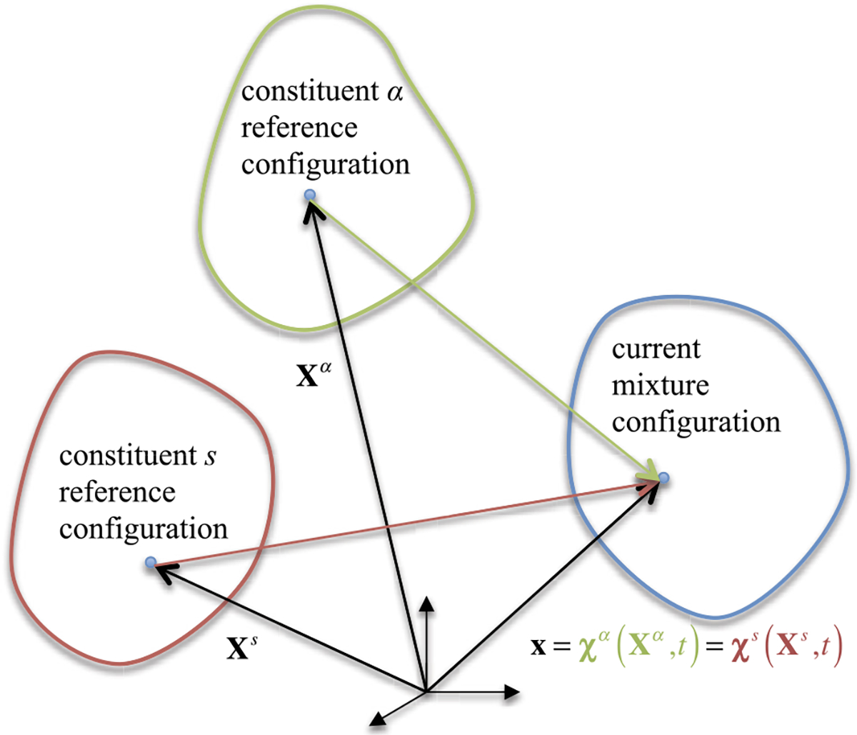
Motion of a mixture and its constituents

The velocity ${\mathbf{V}}^{\alpha }\left({\mathbf{X}}^{\alpha },t\right)$ of constituent $\alpha$ in its material frame is defined as

$${\mathbf{V}}^{\alpha }\left({\mathbf{X}}^{\alpha },t\right)=\frac{\partial {\mathit{\chi }}^{\alpha }\left({\mathbf{X}}^{\alpha },t\right)}{\partial t},$$ (2.1)

whereas the deformation gradient ${\mathbf{F}}^{\alpha }\left({\mathbf{X}}^{\alpha },t\right)$ is defined as

$${\mathbf{F}}^{\alpha }\left({\mathbf{X}}^{\alpha },t\right)=\frac{\partial {\mathit{\chi }}^{\alpha }\left({\mathbf{X}}^{\alpha },t\right)}{\partial {\mathbf{X}}^{\alpha }}.$$ (2.2)

From these relations, the material time derivative of ${\mathbf{F}}^{\alpha }$ in the material frame is

$$\frac{\partial {\mathbf{F}}^{\alpha }\left({\mathbf{X}}^{\alpha },t\right)}{\partial t}=\frac{\partial {\mathbf{V}}^{\alpha }\left({\mathbf{X}}^{\alpha },t\right)}{\partial {\mathbf{X}}^{\alpha }}={\mathbf{L}}^{\alpha }\left({\chi }^{\alpha }\left({\mathbf{X}}^{\alpha },t\right),t\right)\cdot {\mathbf{F}}^{\alpha }\left({\mathbf{X}}^{\alpha },t\right),$$ (2.3)

where

$${\mathbf{L}}^{\alpha }(\mathbf{x},t)=\mathrm{g}\mathrm{r}\mathrm{a}\mathrm{d}{\mathbf{v}}^{\alpha }(\mathbf{x},t)$$ (2.4)

is the spatial gradient of the velocity ${\mathbf{v}}^{\alpha }(\mathbf{x},t)$ of $\alpha$. We may rewrite this expression as ${\dot{\mathbf{F}}}^{\alpha }={\mathbf{L}}^{\alpha }\cdot {\mathbf{F}}^{\alpha }$.

A constrained mixture represents the special case when all solid constituents share the same spatial velocity [30]; this constraint is expressed in the spatial frame as

$${\mathbf{v}}^{\alpha }(\mathbf{x},t)={\mathbf{v}}^s(\mathbf{x},t),$$ (2.5)

where $s$ represents one of the constrained mixture constituents. This relation implies that ${\mathbf{L}}^{\alpha }(\mathbf{x},t)={\mathbf{L}}^s(\mathbf{x},t)$ for all constrained mixture constituents $\alpha$. Note that the respective referential configurations ${\mathbf{X}}^{\alpha }$ of the various constituents $\alpha$ need not be the same, since each constituent may have formed (come into existence as the product of a reaction) at a different time point. For the pair of constituents $\alpha$ and $s$, it follows that $d\mathbf{x}={\mathbf{F}}^{\alpha }\left({\mathbf{X}}^{\alpha },t\right)\cdot d{\mathbf{X}}^{\alpha }={\mathbf{F}}^s\left({\mathbf{X}}^s,t\right)\cdot d{\mathbf{X}}^s$, explicitly establishing the relation between constituent deformation gradients. In this expression, $d{\mathbf{X}}^{\alpha }$ is a differential line element at ${\mathbf{X}}^{\alpha }$ which transforms into $d\mathbf{x};d{\mathbf{X}}^s$ is the line element at ${\mathbf{X}}^s$ that also transforms into $d\mathbf{x}$, where ${\mathbf{X}}^{\alpha }$ and ${\mathbf{X}}^s$ represent those material points of constituents $\alpha$ and $s$ that meet at $\mathbf{x}={\mathit{\chi }}^{\alpha }\left({\mathbf{X}}^{\alpha },t\right)={\mathit{\chi }}^s\left({\mathbf{X}}^s,t\right)$ at the current time $t$. In particular, it may be convenient to identify the reference configuration $s$ as the master reference configuration, ${\mathbf{X}}^s$, so that

$${\mathbf{F}}^s\left({\mathbf{X}}^s,t\right)={\mathbf{F}}^{\alpha }\left({\mathbf{X}}^{\alpha },t\right)\cdot \frac{\partial {\mathbf{X}}^{\alpha }\left({\mathbf{X}}^s\right)}{\partial {\mathbf{X}}^s}\equiv {\mathbf{F}}^{\alpha }\left({\mathbf{X}}^{\alpha },t\right)\cdot {\mathbf{F}}^{\alpha s}\left({\mathbf{X}}^s\right),$$ (2.6)

where ${\mathbf{F}}^{\alpha s}\left({\mathbf{X}}^s\right)=\partial {\mathbf{X}}^{\alpha }\left({\mathbf{X}}^s\right)/\partial {\mathbf{X}}^s$ represents the deformation gradient of $\alpha$ relative to $s$. For example, in a reactive mixture, $s$ may represent the oldest solid constituent. In a constrained mixture, the relation between ${\mathbf{X}}^{\alpha }$ and ${\mathbf{X}}^s$ is invariant in time and ${\mathbf{F}}^{\alpha s}\left({\mathbf{X}}^s\right)$ is a pre-determined spatial mapping that defines the function ${\mathbf{X}}^{\alpha }\left({\mathbf{X}}^s\right)$. In the remainder of this treatment, the time-invariant dependence of ${\mathbf{X}}^{\alpha }$ on ${\mathbf{X}}^s$ is implied for any expression using ${\mathbf{X}}^{\alpha }$. Therefore, the material time derivative of ${\mathbf{F}}^s\left({\mathbf{X}}^s,t\right)$ in (2.6) is ${\dot{\mathbf{F}}}^s\left({\mathbf{X}}^s,t\right)={\dot{\mathbf{F}}}^{\alpha }\left({\mathbf{X}}^{\alpha },t\right)\cdot {\mathbf{F}}^{\alpha s}\left({\mathbf{X}}^s\right)$ and this relation remains consistent with the kinematic relations ${\dot{\mathbf{F}}}^s={\mathbf{L}}^s\cdot {\mathbf{F}}^s$ and ${\dot{\mathbf{F}}}^{\alpha }={\mathbf{L}}^s\cdot {\mathbf{F}}^{\alpha }$. The volume ratios $J^{\alpha }\left({\mathbf{X}}^{\alpha },t\right)=\mathrm{d}\mathrm{e}\mathrm{t}{\mathbf{F}}^{\alpha }\left({\mathbf{X}}^{\alpha },t\right)$ similarly satisfy

$$J^s\left({\mathbf{X}}^s,t\right)=J^{\alpha }\left({\mathbf{X}}^{\alpha },t\right)J^{\alpha s}\left({\mathbf{X}}^s\right),$$ (2.7)

where $J^s\left({\mathbf{X}}^s,t\right)=\mathrm{d}\mathrm{e}\mathrm{t}{\mathbf{F}}^s\left({\mathbf{X}}^s,t\right)$ and $J^{\alpha s}\left({\mathbf{X}}^s\right)=\mathrm{d}\mathrm{e}\mathrm{t}{\mathbf{F}}^{\alpha s}\left({\mathbf{X}}^s\right)$. As discussed in greater detail below, the mapping ${\mathbf{F}}^{\alpha s}\left({\mathbf{X}}^s\right)$ in a constrained mixture must be postulated by constitutive assumption.

Under infinitesimal strain analyses, we note that

$${\mathbf{F}}^{\alpha }\approx \mathbf{I}+{\mathit{\epsilon }}^{\alpha }+{\mathit{\omega }}^{\alpha },$$ (2.8)

where ${\mathit{\epsilon }}^{\alpha }$ is the symmetric infinitesimal strain tensor and $\mathbf{I}+{\mathit{\omega }}^{\alpha }$ is the infinitesimal rotation tensor for constituent $\alpha$. Here, ${\mathit{\omega }}^{\alpha }$ is antisymmetric and its dual vector points along the axis of rotation and its magnitude is the infinitesimal angle of rotation. From a Taylor series expansion of $\mathrm{d}\mathrm{e}\mathrm{t}{\mathbf{F}}^{\alpha }$, it can be shown that

$${\mathit{J}}^{\alpha }\approx 1+\mathrm{tr}{\mathit{\epsilon }}^{\alpha }.$$ (2.9)

Under these conditions, the relation of (2.6) may be rewritten as

$$\mathbf{I}+{\mathit{\epsilon }}^s+{\mathit{\omega }}^s\approx \left(\mathbf{I}+{\mathit{\epsilon }}^{\alpha }+{\mathit{\omega }}^{\alpha }\right)\cdot \left(\mathbf{I}+{\mathit{\epsilon }}^{\alpha s}+{\mathit{\omega }}^{\alpha s}\right).$$ (2.10)

Equating symmetric and antisymmetric parts of this relation and neglecting higher order products produces

$$\begin{array}{c}{\mathit{\epsilon }}^s={\mathit{\epsilon }}^{\alpha s}+{\mathit{\epsilon }}^{\alpha },\\ {\mathit{\omega }}^s={\mathit{\omega }}^{\alpha s}+{\mathit{\omega }}^{\alpha }.\end{array}$$ (2.11)

Just like ${\mathbf{F}}^{\alpha s}$, the relative strain ${\mathit{\epsilon }}^{\alpha s}$ and relative rotation ${\mathit{\omega }}^{\alpha s}$ are temporally invariant measures which are prescribed based on constitutive assumptions. In particular, when all constituents $\alpha$ are assumed to share a common reference configuration with the master constituent $s$, it follows that ${\mathbf{F}}^{\alpha s}=\mathbf{I}$ and ${\mathit{\epsilon }}^{\alpha s}=0$.

2.2. Apparent Density

The apparent density ${\rho }^{\alpha }$ of mixture constituent $\alpha$ is defined as

$${\rho }^{\alpha }\left(\mathbf{x},t\right)=\frac{d{m}^{\alpha }}{dV},$$ (2.12)

where $d{m}^{\alpha }$ is the mass of constituent $\alpha$ in the mixture elemental volume $dV$, both given in the current configuration. The apparent density of $\alpha$ may also be called the mass concentration of $\alpha$. In a general analysis, both $d{m}^{\alpha }$ and $dV$ may evolve with time.

We may also define the referential apparent density ${\rho }_r\left({\mathbf{X}}^{\alpha },t\right)$ of constituent $\alpha$ as

$${\rho }_r^{\alpha }\left({\mathbf{X}}^{\alpha },t\right)=\frac{d{m}^{\alpha }}{d{V}_r},$$ (2.13)

where $d{V}_r$ is the mixture volume in the reference configuration of the master constituent $s$ (Fig. 1). This definition is consistent with the adoption of the reference configuration of the master constituent as that of the mixture domain. For example, in a finite element model of a reactive mixture, the undeformed mesh represents the stress-free configuration of constituent $s$. Since $dV/d{V}_r=J^s$, the relation between ${\rho }^{\alpha }(\mathbf{x},t)$ and ${\rho }_r^{\alpha }\left({\mathbf{X}}^{\alpha },t\right)$ is

$${\rho }_r^{\alpha }\left({\mathbf{X}}^{\alpha },t\right)={\rho }^{\alpha }\left({\chi }^s\left({\mathbf{X}}^s,t\right),t\right)J^s\left({\mathbf{X}}^s,t\right).$$ (2.14)

Example 1

Consider a soft hydrated tissue such as articular cartilage, which may be modeled as a mixture of a collagen fibrillar matrix, proteoglycans, water, sodium and chloride ions. The collagen-proteoglycan mixture may be modeled as a constrained solid mixture, since the proteoglycan macromolecules are typically enmeshed within, and bound to the collagen. The remaining constituents are fluids that may transport through the porous, permeable collagen-proteoglycan solid matrix. The macroscopic boundaries of the fibrillar collagen matrix define the boundaries of a cartilage tissue specimen, as collagen is the most abundant solid constituent; in contrast, proteoglycan macromolecules are interspersed within the collagen matrix. Therefore, the collagen constituent is the natural choice of master constituent in a cartilage mixture model. Since fluids do not have a natural stress-free configuration, they represent less convenient choices when defining a master constituent.

Other common definitions of concentration exist, most notably the molar concentration $c^{\alpha }$ of constituent $\alpha$, given by

$$c^{\alpha }=\frac{d{n}^{\alpha }}{dV},$$ (2.15)

where $d{n}^{\alpha }$ is the number of moles of $\alpha$ in the elemental volume $dV$. We may relate mass and molar concentrations using

$${\rho }^{\alpha }=M^{\alpha }{c}^{\alpha },$$ (2.16)

where $M^{\alpha }=d{m}^{\alpha }/d{n}^{\alpha }$ is the molar mass of constituent $\alpha$, which is an invariant material property of constituent $\alpha$.

2.3. Axiom of Mass Balance for Each Constituent

The axiom of mass balance may be derived for constituent $\alpha$ in integral form using a control volume $V$. The time rate of change of mass of $\alpha$ in the control volume is equal to the rate at which the mass of $\alpha$ is convected into $V$ across its control surface $\partial V$ and the rate at which mass is supplied to $\alpha$ from reactions with other mixture constituents,

$$\frac{d}{dt}{\int }_V{\rho }^{\alpha }dV=-{\int }_{\partial V}{\rho }^{\alpha }\left({\mathbf{v}}^{\alpha }\cdot \mathbf{n}\right)dS+{\int }_V{\hat{\rho }}^{\alpha }dV.$$ (2.17)

Here, ${\hat{\rho }}^{\alpha }(\mathbf{x},t)$ is the mass density supply (with units of mass per volume, per time) to $\alpha$ from all other constituents resulting from reactions. The mass supply is a function of state that needs to be defined with a suitable constitutive relation. Using the divergence theorem, this integral form may be converted to the differential form

$$\frac{\partial {\rho }^{\alpha }}{\partial t}+\mathrm{d}\mathrm{i}\mathrm{v}\left({\rho }^{\alpha }{\mathbf{v}}^{\alpha }\right)={\hat{\rho }}^{\alpha }.$$ (2.18)

Expanding the expression in the divergence operator and defining the material time derivative in the spatial frame, following constituent $\alpha$, as

$$\frac{D^{\alpha }(\cdot )}{Dt}=\frac{\partial (\cdot )}{\partial t}+\mathrm{g}\mathrm{r}\mathrm{a}\mathrm{d}(\cdot )\cdot {\mathbf{v}}^{\alpha },$$ (2.19)

we may rewrite the mass balance for constituent $\alpha$ as

$$\frac{D^{\alpha }{\rho }^{\alpha }}{Dt}+{\rho }^{\alpha }\mathrm{d}\mathrm{i}\mathrm{v}{\mathbf{v}}^{\alpha }={\hat{\rho }}^{\alpha }.$$ (2.20)

For the constituents $\alpha$ of a constrained mixture, since there is no relative motion between $\alpha$ and $s$, we may express the integral form of the mass balance in the material frame of the master constituent $s$ as

$$\frac{d}{dt}{\int }_{V_r}{\rho }_r^{\alpha }\left({\mathbf{X}}^{\alpha },t\right)d{V}_r={\int }_{V_r}{\hat{\rho }}_r^{\alpha }\left({\mathbf{X}}^{\alpha },t\right)d{V}_r,$$ (2.21)

where

$${\hat{\rho }}_r^{\alpha }\left({\mathbf{X}}^{\alpha },t\right)=J^s\left({\mathbf{X}}^s,t\right){\hat{\rho }}^{\alpha }\left({\chi }^s\left({\mathbf{X}}^s,t\right),t\right)$$ (2.22)

may be called the referential mass density supply to constituent $\alpha$. Thus, the differential form of the mass balance in the material frame is given by

$${\dot{\rho }}_r^{\alpha }\equiv \frac{\partial {\rho }_r^{\alpha }\left({\mathbf{X}}^{\alpha },t\right)}{\partial t}={\hat{\rho }}_r^{\alpha }\left({\mathbf{X}}^{\alpha },t\right).$$ (2.23)

Equation (2.23) shows that ${\rho }_r^{\alpha }$ remains time-invariant for non-reactive constituents $\alpha$ in a mixture, since ${\hat{\rho }}_r^{\alpha }=0$ for those constituents. From the definition given in (2.13), it becomes evident that ${\rho }_r^{\alpha }$ evolves only as a result of changes in $d{m}^{\alpha }$, since $d{V}_r$ is constant by definition. In contrast, looking at the definition of ${\rho }^{\alpha }$ in (2.12), we find that ${\rho }^{\alpha }$ of a constrained mixture constituent may evolve as a result of reactions (evolving $d{m}^{\alpha }$) and deformations (evolving $dV$). Therefore, in contrast to ${\rho }^{\alpha },{\rho }_r^{\alpha }$ is a more convenient choice of state variable when modeling reactive constrained mixtures, since it can track the evolution of the mass content of $\alpha$ occurring exclusively in response to reactions, whereas the complete state of deformation of that constituent may be tracked using ${\mathbf{F}}^{\alpha }$.

The mass balance for the mixture is obtained by summing the mass balance in Eq. (2.18) over all constituents. The axiom of mixtures states that the governing equations for the mixture should have the same form as those of a single, pure substance (a single, non-reactive constituent $\alpha$). As shown previously [4, 12, 13, 21], it follows that the mass supplies must satisfy

$$\sum _{\alpha }{\hat{\rho }}^{\alpha }=0,$$ (2.24)

implying that the rate at which mass is lost from reactants must be matched by the rate at which mass is added to products, in all reactions occurring in the mixture.

2.4. Reactive Mixtures

Reactions may occur among the constituents of a mixture which result in a temporal evolution of the mass content of reactants and products. A forward reaction between mixture constituents may be written down as

$$\sum _{\alpha }{v}_R^{\alpha }{ℰ}^{\alpha }\to \sum _{\alpha }{v}_P^{\alpha }{ℰ}^{\alpha },$$ (2.25)

where ${ℰ}^{\alpha }$ is the chemical (molecular) species associated with constituent $\alpha ,v_R^{\alpha }$ represents the stoichiometric coefficient of reactant $\alpha$ and $v_P^{\alpha }$ is that of the corresponding product. Similarly, a reversible reaction may be written as

$$\sum _{\alpha }{v}_R^{\alpha }{ℰ}^{\alpha }\rightleftharpoons \sum _{\alpha }{v}_P^{\alpha }{ℰ}^{\alpha }.$$ (2.26)

The summations are taken over all mixture constituents, though constituents that are not reactants in that particular reaction will have $v_R^{\alpha }=0$, and those that are not products will have $v_P^{\alpha }=0$. The stoichiometry of the reaction imposes constraints on the mass supplies such that we may define a molar production rate $\hat{\zeta }$ (units of moles per volume, per time),

$${\hat{\rho }}^{\alpha }=M^{\alpha }{v}^{\alpha }\hat{\zeta },$$ (2.27)

where

$$v^{\alpha }=v_P^{\alpha }-v_R^{\alpha }$$ (2.28)

is the net stoichiometric coefficient of $\alpha$ in the reaction. The relation (2.27) may be substituted into the constraint on mass supplies, Eq. (2.24) to produce

$$\sum _{\alpha }{M}^{\alpha }{v}^{\alpha }=0.$$ (2.29)

This relation may be recognized as the classical requirement to balance the molar mass of reactants and products in a reaction. Thus, the constraint resulting from the axiom of mixtures produces a classical outcome when applied to the mass balance. For constrained mixture constituents, the relation (2.27) may also be written as

$${\hat{\rho }}_r^{\alpha }=M^{\alpha }{v}^{\alpha }{\hat{\zeta }}_r,$$ (2.30)

where ${\hat{\zeta }}_r=J^s\hat{\zeta }$.

Example 2

In the reaction

$${\mathrm{H}}_2{\mathrm{S}\mathrm{O}}_4\to 2{\mathrm{H}}^{+}+{\mathrm{S}\mathrm{O}}_4^{2-},$$

we have a total of three constituents, $\alpha ={\mathrm{H}}_2{\mathrm{S}\mathrm{O}}_4,{\mathrm{H}}^{+},{\mathrm{S}\mathrm{O}}_4^{2-}$. Their stoichiometric coefficients are given by

$$v_R^{{\mathrm{H}}_2{\mathrm{S}\mathrm{O}}_4}=1,v_P^{{\mathrm{H}}_2{\mathrm{S}\mathrm{O}}_4}=0,v^{{\mathrm{H}}_2{\mathrm{S}\mathrm{O}}_4}=-1,$$

$$v_R^{{\mathrm{H}}^{+}}=0,v_P^{{\mathrm{H}}^{+}}=2,v^{{\mathrm{H}}^{+}}=2,$$

$$v_R^{{\mathrm{S}\mathrm{O}}_4^{2-}}=0,v_P^{{\mathrm{S}\mathrm{O}}_4^{2-}}=1,v^{{\mathrm{S}\mathrm{O}}_4^{2-}}=1.$$

Therefore, based on Eq. (2.27), we find that

$${\hat{\rho }}^{{\mathrm{H}}_2{\mathrm{S}\mathrm{O}}_4}=-M^{{\mathrm{H}}_2{\mathrm{S}\mathrm{O}}_4}\hat{\zeta },{\hat{\rho }}^{{\mathrm{H}}^{+}}=2M^{{\mathrm{H}}^{+}}\hat{\zeta },{\hat{\rho }}^{{\mathrm{S}\mathrm{O}}_4^{2-}}=M^{{\mathrm{S}\mathrm{O}}_4^{2-}}\hat{\zeta },$$

and the constraint of Eq. (2.29) reduces to

$$-M^{{\mathrm{H}}_2{\mathrm{S}\mathrm{O}}_4}+2M^{{\mathrm{H}}^{+}}+M^{{\mathrm{S}\mathrm{O}}_4^{2-}}=0.$$

2.5. Chemical Kinetics

The mass balance equations for mixture constituents require the specification of constitutive relations for the mass supplies ${\hat{\rho }}^{\alpha }$. Equation (2.27) shows that it suffices to provide a single constitutive relation for the molar production rate $\hat{\zeta }$. Constitutive relations are generally formulated based on experimental observations. For chemical reactions, a commonly used constitutive relation is the law of mass action [46]. In this section we adopt the form of these constitutive relations which employs referential mass densities and density supplies, convenient for the analysis of constrained mixtures.

For forward reactions, the law of mass action may take the form

$${\hat{\zeta }}_r=k\prod _{\alpha }{\left(c_r^{\alpha }\right)}^{v_R^{\alpha }},c_r^{\alpha }\equiv \frac{{\rho }_r^{\alpha }}{M^{\alpha }},$$ (2.31)

where $k$ is the specific reaction rate. For reversible reactions, the net molar production rate is

$${\hat{\zeta }}_r={\hat{\zeta }}_F-{\hat{\zeta }}_R,$$ (2.32)

where

$$\begin{array}{l}{\hat{\zeta }}_F=k_F\prod _{\alpha }{\left(c_r^{\alpha }\right)}^{{\nu }_R^{\alpha }},\\ {\hat{\zeta }}_R=k_R\prod _{\alpha }{\left(c_r^{\alpha }\right)}^{{\nu }_P^{\alpha }},\end{array}$$ (2.33)

represent forward and reverse production rates. We may combine these relations as

$${\hat{\zeta }}_r={\hat{\zeta }}_F\left[1-\frac{k_R}{k_F}\prod _{\alpha }{\left(c_r^{\alpha }\right)}^{v^{\alpha }}\right],$$ (2.34)

where the ratio of forward and reversible specific reaction rates reduces to the equilibrium constant $K_c$ when the reaction has reached steady state,

$${\left.\frac{k_F}{k_R}\right|}_{{\hat{\zeta }}_r=0}\equiv K_c.$$ (2.35)

Example 3

We reprise the reaction of Example 2 and use the law of mass action in Eq. (2.31),

$${\hat{\zeta }}_r=k\frac{{\rho }_r^{{\mathrm{H}}_2{\mathrm{S}\mathrm{O}}_4}}{M^{{\mathrm{H}}_2{\mathrm{S}\mathrm{O}}_4}}.$$

This expression may be substituted into (2.30) to produce ${\hat{\rho }}_r^{{\mathrm{H}}_2{\mathrm{S}\mathrm{O}}_4}$, which may then be substituted into the mass balance relation (2.23)

$$\frac{\partial {\rho }_r^{{\mathrm{H}}_2{\mathrm{S}\mathrm{O}}_4}}{\partial t}=-M^{{\mathrm{H}}_2{\mathrm{S}\mathrm{O}}_4}{\hat{\zeta }}_r=-k{\rho }_r^{{\mathrm{H}}_2{\mathrm{S}\mathrm{O}}_4}.$$

This linear differential equation may be integrated subject to the homogeneous initial condition ${\rho }_r^{{\mathrm{H}}_2{\mathrm{S}\mathrm{O}}_4}\left({\mathbf{X}}^s,0\right)={\rho }_0^{{\mathrm{H}}_2{\mathrm{S}\mathrm{O}}_4}$ to produce

$${\rho }_r^{{\mathrm{H}}_2{\mathrm{S}\mathrm{O}}_4}\left({\mathbf{X}}^s,t\right)={\rho }_0^{{\mathrm{H}}_2{\mathrm{S}\mathrm{O}}_4}{e}^{-kt},$$

showing that the concentration of the reactant decays exponentially with a time constant $1/k$. Accordingly, this type of response is called a first-order reaction and we find that the specific reaction rate controls the temporal response. Given this solution, it follows that

$${\hat{\zeta }}_r=k\frac{{\rho }_0^{{\mathrm{H}}_2{\mathrm{S}\mathrm{O}}_4}}{M^{{\mathrm{H}}_2{\mathrm{S}\mathrm{O}}_4}}{e}^{-kt},$$

which may be used to similarly solve for the concentrations of the products,

$$\frac{{\rho }_r^{{\mathrm{H}}^{+}}\left({\mathbf{X}}^s,t\right)}{M^{{\mathrm{H}}^{+}}}=\frac{{\rho }_0^{{\mathrm{H}}^{+}}}{M^{{\mathrm{H}}^{+}}}+2\frac{{\rho }_0^{{\mathrm{H}}_2{\mathrm{S}\mathrm{O}}_4}}{M^{{\mathrm{H}}_2{\mathrm{S}\mathrm{O}}_4}}\left(1-e^{-kt}\right),$$

$$\frac{{\rho }_r^{{\mathrm{S}\mathrm{O}}_4^{2-}}\left({\mathbf{X}}^s,t\right)}{M^{{\mathrm{S}\mathrm{O}}_4^{2-}}}=\frac{{\rho }_0^{{\mathrm{S}\mathrm{O}}_4^{2-}}}{M^{{\mathrm{S}\mathrm{O}}_4^{2-}}}+\frac{{\rho }_0^{{\mathrm{H}}_2{\mathrm{S}\mathrm{O}}_4}}{M^{{\mathrm{H}}_2{\mathrm{S}\mathrm{O}}_4}}\left(1-e^{-kt}\right).$$

Example 4

Receptor-ligand kinetics is a classical example of a reversible reaction in biochemistry, where a ligand binds to a receptor to produce a receptor-ligand complex. The reaction is reversible, implying that the complex may also dissociate back into its constituents. The forward and reverse reactions may proceed at different rates. Let the receptor be denoted with $\mathrm{R}$ and the ligand with $\mathrm{L}$, whereas the receptor-ligand complex is $\mathrm{C}$. The reaction is given by

$$\mathrm{R}+\mathrm{L}\rightleftharpoons \mathrm{C}.$$

The initial concentrations are $c_r^{\mathrm{R}}\left({\mathbf{X}}^s,0\right)=c_0^{\mathrm{R}},c_r^{\mathrm{L}}\left({\mathbf{X}}^s,0\right)=c_0^{\mathrm{L}}$, and $c_r^{\mathrm{C}}\left({\mathbf{X}}^s,0\right)=0$. The molar production rate is

$${\hat{\zeta }}_r=k_F{c}_r^{\mathrm{R}}{c}_r^{\mathrm{L}}-k_R{c}_r^{\mathrm{C}}.$$

From mass balance it follows that $c_r^{\mathrm{R}}=c_0^R-c_r^{\mathrm{C}}$ and $c_r^{\mathrm{L}}=c_0^{\mathrm{L}}-c_r^{\mathrm{C}}$. Therefore,

$${\hat{\zeta }}_r=k_F\left(c_0^R-c_r^{\mathrm{C}}\right)\left(c_0^{\mathrm{L}}-c_r^{\mathrm{C}}\right)-k_R{c}_r^{\mathrm{C}},$$

and the mass balance for the complex becomes

$$\frac{\partial c_r^{\mathrm{C}}}{\partial t}=k_F\left(c_0^R-c_r^{\mathrm{C}}\right)\left(c_0^{\mathrm{L}}-c_r^{\mathrm{C}}\right)-k_R{c}_r^{\mathrm{C}}.$$

The solution to this nonlinear ordinary differential equation is

$$c_r^{\mathrm{C}}\left({\mathbf{X}}^s,t\right)=c_0-\chi \tanh \left(k_F\chi t+{\tanh }^{-1}\frac{c_0}{\chi }\right),$$

where

$$c_0=\frac{1}{2}\left(c_0^{\mathrm{L}}+c_0^{\mathrm{R}}+K_d\right),K_d=\frac{k_R}{k_F},\chi =\sqrt{c_0^2-c_0^{\mathrm{R}}{c}_0^{\mathrm{L}}}.$$

At steady state the solution is

$$c_r^{\mathrm{C}}\left({\mathbf{X}}^s,t\to \mathrm{\infty }\right)=c_0-\chi =c_0-c_0\sqrt{1-\frac{c_0^{\mathrm{R}}{c}_0^{\mathrm{L}}}{c_0^2}}.$$

In the limit when $c_0^{\mathrm{R}}{c}_0^{\mathrm{L}}/c_0^2\ll 1$, i.e., when the initial ligand concentration or the initial receptor concentration is much smaller than the dissociation constant $K_d$, this solution reduces to

$$c_r^{\mathrm{C}}\left({\mathbf{X}}^s,t\to \mathrm{\infty }\right)\approx \frac{1}{2}\frac{c_0^{\mathrm{R}}{c}_0^{\mathrm{L}}}{c_0}=\frac{c_0^{\mathrm{R}}{c}_0^{\mathrm{L}}}{c_0^{\mathrm{L}}+c_0^{\mathrm{R}}+K_d}.$$

2.6. Interstitial Solid Growth and Remodeling

Interstitial growth implies solid mass deposition within a porous mixture. This type of growth is not necessarily biological. For example, a metallic porous filter may be imbibed with a fluid that causes metal oxidation, so that the mass of metal decreases while that of the metal oxide increases throughout the entire filter domain. In the case of biological tissues, biochemical reactions may occur that are not necessarily driven directly by cell activity, such as binding of exogenous growth factors to the extracellular matrix. Conversely, cells may directly process soluble reactants to produce extracellular matrix products in a process variably called growth or remodeling. In a generic sense, this type of reaction may be written as

$$\text{cells}+\text{nutrients}\to \text{cells}+\text{solid}\text{matrix.}$$

For such growth processes, the law of mass action may or may not be directly applicable, especially when a multitude of reactions are taking place simultaneously, whose aggregate response on solid matrix production is not reducible to the functional form of the law of mass action. Furthermore, when dealing with biological tissues where solid deformation occurs, the growth process may be significantly influenced by such deformations and their history over an extended period of intermittent loading. Therefore, constitutive modeling of such growth processes may be reformulated to reflect experimental observations at a more global level, rather than the intricate details of individual chemical reactions.

In the sections below we examine basic problems in tissue growth and remodeling. Interstitial growth implies that the referential apparent density ${\rho }_r^{\alpha }$ of a solid constituent increases over time; this type of growth leads to an increase in the mass of constituent $\alpha$ but does not necessarily produce changes to the overall tissue dimensions. For example, in tissue engineering where cells are seeded within a scaffold, the cells may synthesize solid matrix that fills the scaffold interstitial space, without altering the overall dimensions of the engineered construct. If the scaffold is degradable, its loss of mass (e.g., solubilization) represents negative growth.

In contrast to growth, tissue remodeling may be viewed as the effect of reactions that alter the mass content of various solid constituents, without an obligatory net change in total solid mass content. This distinction between growth and remodeling is semantic; effectively, both phenomena involve reactions that alter the mass content of various solid constituents.

In biomechanics, it is common to model biological soft tissues as being nearly incompressible. This choice of material behavior is sometimes convenient for simplifying analyses of tissue responses, as in studies where two-dimensional strain measurements are performed on the surface of a tissue layer and the strain through the layer thickness is deduced from the assumption that the response is isochoric. It is useful to understand when this assumption may be valid, especially in the context of reactive mixtures where growth and resorption of solid constituents alter the tissue porosity.

The best evidence available to us is arguably from studies of articular cartilage, which has been alternatively modeled as an incompressible or nearly incompressible elastic solid [1, 20] or a porous-permeable biphasic material (a solid-fluid mixture or poroelastic material) [2, 41]. Cartilage has a porosity ranging from 90 to 65 percent, decreasing with depth from the articular surface, and with age [56]. The interstitial fluid of cartilage consists primarily of water and inorganic salts; this fluid may flow within cartilage since its pores communicate, as evidenced by direct measurements of its hydraulic permeability [39]. Experiments have shown that loading of articular cartilage causes its interstitial fluid to pressurize; this pressure subsides when the loading remains static for a sustained period of time, as the pressurized fluid flows away from the loaded region [43]. Excellent agreement has been found between direct measurements of the interstitial fluid pressure and predictions from the biphasic theory [44, 52, 53], which assumes that each mixture constituent (solid and fluid) is intrinsically incompressible, though the mixture (defined over the domain of the porous solid matrix) may change in volume with time as the fluid flows through it [41]. The assumption of intrinsic incompressibility of each constituent was validated from direct experimental measurements of cartilage subjected to hydrostatic pressures up to 12 MPa [11].

The biphasic theory predicts that the instantaneous response of cartilage to loading is isochoric, since the interstitial fluid cannot instantaneously flow out of the mixture due its frictional interactions with the solid [2, 6, 38]. This behavior has been verified from experimental measurements of Poisson’s ratio in cartilage subjected to rapid loading under small strains, which produced values approaching 0.5 [28, 65]. Moreover, the biphasic theory predicts that the equilibrium response of cartilage, achieved when the interstitial fluid pressure and flow have subsided, is equivalent to that of a compressible elastic solid [2, 38, 41]. Experimental measurements of Poisson’s ratio under equilibrium conditions have yielded values as low as 0.02 [16]. This very low value implies that the porous solid matrix has negligible lateral expansion upon axial compression, with the reduction in volume occurring in the pore space. In contrast, a biphasic material with zero porosity (no fluid content), or with non-communicating pores, is intrinsically incompressible since no fluid may enter or leave the tissue.

In reality, interstitial fluid may also be exchanged with hydrated biological tissues via osmotic mechanisms. Experiments on cartilage, intervertebral disc, arterial wall and cornea have shown that they swell or shrink in response to osmotic loading, when the salt concentration of the surrounding fluid bath is altered [10, 14, 16, 40, 57]. Therefore, the assumption that these tissues may be modeled as incompressible solids that cannot change in volume should be adopted carefully, as it is valid only under special circumstances: As long as the interstitial fluid has not had sufficient time to flow into or out of the porous solid matrix in response to mechanical or osmotic loading, or growth and remodeling processes that alter the porosity, it is reasonable to assume that the response to mechanical loading will be isochoric.

Conversely, since growth and remodeling may alter the solid matrix porosity of a biological tissue, as also illustrated in our prior theoretical study of cell growth [7], it would be unreasonable to illustrate this mechanism with examples that use a value of 0.5 for Poisson’s ratio. Therefore, in the examples that follow, a value of zero is selected for simplicity. This value does not preclude isochoric responses under rapid loading and unloading when the pore space is filled with interstitial fluid [2, 6, 38].

2.6.1. Bone Remodeling in Response to Loading

Bone is known to respond to loading according to Wolff’s law, whereby bone mass increases or decreases when loading deviates from a set point. We may generically represent these reactions as

$$\text{cells}+\text{nutrients}\stackrel{\text{loading}}{\to }\text{cells}+\text{solid}\text{matrix},$$ (2.36)

$$\text{cells}+\text{solid}\text{matrix}\stackrel{\text{unloading}}{\to }\text{cells}+\text{soluble}\text{waste}\text{products}.$$ (2.37)

In this case the first reaction is only triggered when the loading exceeds the set point, whereas the second reaction is exclusively triggered when the loading falls below the threshold. The cells involved in these processes may even be different; in the case of bone, matrix synthesis is driven by osteoblasts whereas matrix degradation is performed by osteoclasts.

For trabecular bone remodeling, Huiskes and co-workers proposed the following constitutive relation to embody Wolff’s law,

$${\hat{\rho }}_r^s=B\left(\frac{{\Psi }_r}{{\rho }_r^s}-{\psi }_0\right),$$ (2.38)

where ${\Psi }_r$ is the strain energy density in the bone, ${\psi }_0$ is the specific strain energy at the set point, and $B$ controls the remodeling rate [29, 63]. This constitutive relation, which responds indiscriminately to tensile, compressive and shear loading, may be substituted into the mass balance (2.23) to solve for the evolving apparent bone density ${\rho }_r^s$,

$$\frac{\partial {\rho }_r^s}{\partial t}=B\left(\frac{{\Psi }_r}{{\rho }_r^s}-{\psi }_0\right).$$ (2.39)

An increase in ${\rho }_r^s$ implies that existing trabeculae become thicker, or more trabeculae form, within a given trabecular bone region, thus decreasing the corresponding pore volume. Conversely, a decrease in ${\rho }_r^s$ implies thinning or resorbing trabeculae, leading to increased porosity.

For a well-posed problem it is necessary to propose a constitutive relation for the free energy density of the solid. For example, we may idealize bone as a linear elastic solid. For a one-dimensional analysis, the stress-strain relation is $\sigma =E\epsilon$ where $E$ is Young’s modulus, so that

$${\Psi }_r=\frac{1}{2}\sigma \epsilon =\frac{1}{2}E{\epsilon }^2=\frac{{\sigma }^2}{2E}.$$ (2.40)

Experimentally, Carter and Hayes [15] found that the strength of trabecular bone varied as a power-law of its apparent density, and a similar relation has been adopted for its Young’s modulus [22, 63],

$$E=c{\left({\rho }_r^s\right)}^{\gamma },$$ (2.41)

where $c$ and $\gamma$ are material parameters obtained empirically. We may now analyze the problem of uniaxial loading of a bar as a canonical problem in this remodeling framework, which may be representative of a long bone such as the femur or humerus. When the bar is subjected to a prescribed normal traction $\sigma$, we use the form ${\Psi }_r={\sigma }^2/2E$ in (2.40), so that the only unknown is the density ${\rho }_r^s$ appearing in the expression for $E$ in (2.41). Substituting these relations above now produces a differential equation that depends on the known state of stress as well as the unknown bone density ${\rho }_r^s$,

$$\frac{\partial {\rho }_r^s}{\partial t}=B\left(\frac{{\sigma }^2}{2c{\left({\rho }_r^s\right)}^{\gamma +1}}-{\psi }_0\right).$$ (2.42)

This equation governs the remodeling of bone in response to loading. Conversely, had the bar been subjected to a prescribed normal strain $\epsilon$, we would have used ${\Psi }_r=E{\epsilon }^2/2$ in (2.40), so that (2.39) would instead reduce to

$$\frac{\partial {\rho }_r^s}{\partial t}=B\left(\frac{1}{2}c{\left({\rho }_r^s\right)}^{\gamma -1}{\epsilon }^2-{\psi }_0\right).$$ (2.43)

Example 5

Consider a bar with initial uniform density ${\rho }_r^s(x,t)={\rho }_0^s$, subjected to a constant traction $\sigma \left(t\right)={\sigma }_0$ on both ends.¹ The transient solution to the above differential equation is most conveniently obtained numerically. However, the response at steady state is easily evaluated by letting $\partial {\rho }_r^s/\partial t=0$ to produce

$${\rho }_{\mathrm{\infty }}^s=\underset{t\to \mathrm{\infty }}{\mathrm{l}\mathrm{i}\mathrm{m}}{\rho }_r^s(x,t)=\sqrt[\gamma +1]{\frac{{\sigma }_0^2}{2c{\psi }_0}}.$$ (2.44)

We conclude that the apparent density remodels from ${\rho }_0^s$ to the new equilibrium value given above, determined by the material parameters $c,\gamma$, and ${\psi }_0$, and the prescribed traction ${\sigma }_0$. This formula shows that the bone density increases with increasing applied stress ${\sigma }_0$; though the formula suggests no limit on its upper bound, in reality ${\rho }_r^s$ reaches a maximum value when all the pore space has been filled with bone matrix, producing a value essentially equivalent to the density of cortical bone. This solution also shows that bone density decreases with increasing set point value ${\psi }_0$. This type of prediction suggests that a disease such as osteoporosis, a complex metabolic bone disease that leads to loss of bone density over time, may be simulated in a growth and remodeling analysis by altering the set point ${\psi }_0$ with disease progression. Effectively, this would indicate that bone cells have become less sensitive to mechanical stimuli, requiring a higher threshold for producing a response comparable to healthy bone.

As a special case, the transient response when ${\sigma }_0=0$ reduces to ${\rho }_r^s(x,t)={\rho }_0^s-B{\psi }_{0}t$, a linear decrease which remains valid until ${\rho }_r^s$ reduces to 0. In general, the rate of remodeling is given directly by the mass balance relation (2.42), which shows that it is proportional to $B$ but evolves with time; at $t=0$ the characteristic time constant $\tau$ for remodeling is

$$\tau =\frac{{\rho }_0^s}{B(\frac{{\sigma }_0^2}{2c{\left({\rho }_0^s\right)}^{\gamma +1}}-{\psi }_0)}.$$ (2.45)

Letting ${\tilde{\rho }}_r^s={\rho }_r^s/{\rho }_0^s$ and $\tilde{t}=t/\tau$, we may non-dimensionalize the differential equation (2.42) as

$$\frac{\partial {\tilde{\rho }}_r^s}{\partial \tilde{t}}=\frac{1}{1-r}\left(\frac{1}{{\left({\tilde{\rho }}_r^s\right)}^{\gamma +1}}-r\right),r={\left(\frac{{\rho }_0^s}{{\rho }_{\mathrm{\infty }}^s}\right)}^{\gamma +1}.$$ (2.46)

The initial condition is ${\tilde{\rho }}_r^s(x,0)=1$. This form is more suitable for numerical implementation and select responses are illustrated in Fig. 2.

Fig. 2.

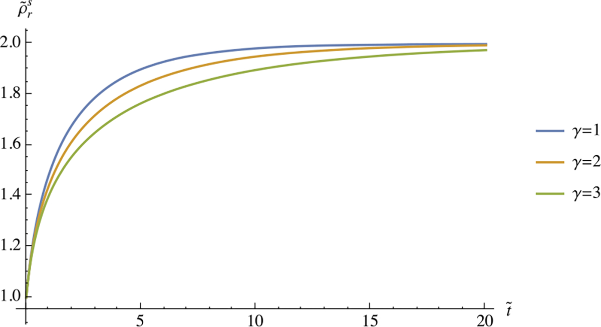
Transient response of ${\tilde{\rho }}_r^s$ versus $\tilde{t}$ in Example 5, using three different values of $\gamma$, with ${\rho }_0^s/{\rho }_{\mathrm{\infty }}^s=1/2$

Example 6

If we allow the traction $\sigma$ to vary cyclically over time with a period $T$, e.g., $\sigma \left(t\right)=\sqrt{2}{\sigma }_0\mathrm{s}\mathrm{i}\mathrm{n}(2\pi t/T)$, the temporal evolution of ${\rho }_r^s$ will also vary cyclically. In a long bone for example, this type of cyclical loading may arise from locomotion and $T$ may be on the order of one second. The non-dimensional form of the differential equation (2.42) becomes

$$\frac{\partial {\tilde{\rho }}_r^s}{\partial \tilde{t}}=\frac{1}{1-r}\left(\frac{2}{{\left({\tilde{\rho }}_r^s\right)}^{\gamma +1}}{\mathrm{s}\mathrm{i}\mathrm{n}}^2\left(2\pi \frac{\tau }{T}\tilde{t}\right)-r\right).$$

An examination of this equation shows that the influence of cyclical loading will be negligible when the period $T$ is much shorter than the characteristic remodeling time $\tau$, which is typical of biological tissue remodeling. Numerical examples are illustrated in Fig. 3.

Fig. 3.

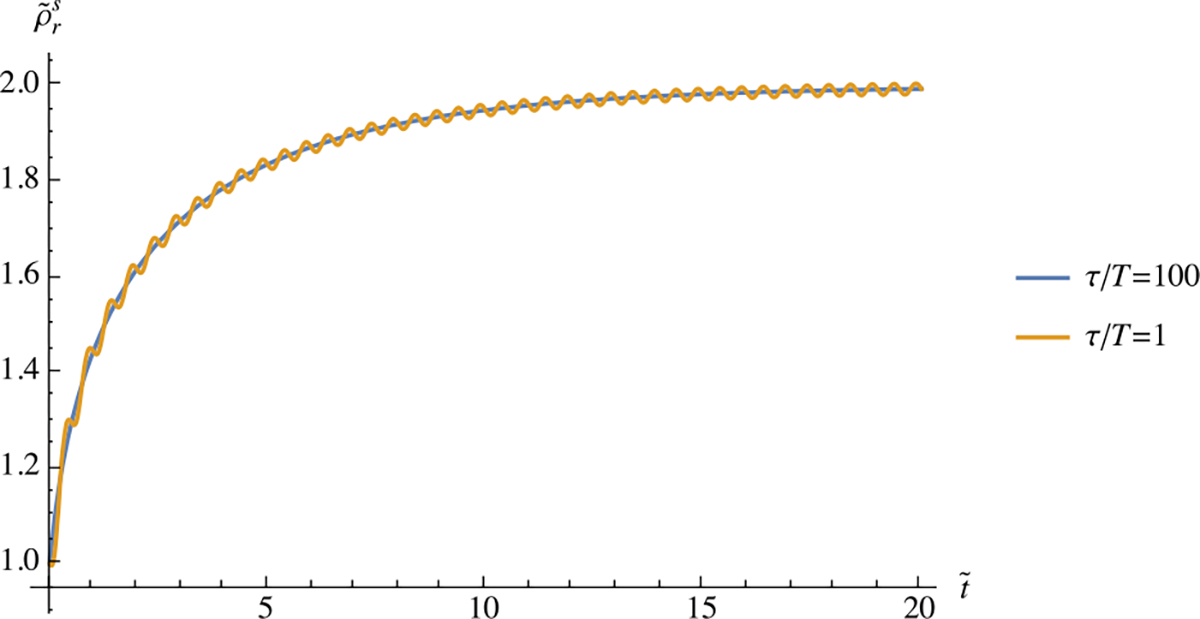
Transient response of ${\tilde{\rho }}_r^s$ versus $\tilde{t}$ in Example 6, using two different values of $\tau /T$, with ${\rho }_0^s/{\rho }_{\mathrm{\infty }}^s=1/2$ and $\gamma =2$. The effect of cyclical loading is negligible when $\tau /T\gg 1$

Example 7

Finally, consider a thick-walled cylindrical tube with inner radius $a$ and outer radius $b$, subjected to an internal pressure $p_0$. This type of geometry may represent an artery for example. In a cylindrical coordinate system, the state of stress is [54]

$$\left[\mathit{\sigma }\right]=\left[\begin{array}{ccc}{\sigma }_{rr}& 0& 0\\ 0& {\sigma }_{\theta \theta }& 0\\ 0& 0& 0\end{array}\right],$$ (2.47a)

where

$${\sigma }_{rr}=\frac{a^2{p}_0}{b^2-a^2}\left(1-\frac{b^2}{r^2}\right),{\sigma }_{\theta \theta }=\frac{a^2{p}_0}{b^2-a^2}\left(1+\frac{b^2}{r^2}\right),a\le r\le b.$$ (2.47b)

For a linear isotropic elastic solid, assuming that Poisson’s ratio is zero for simplicity, the free energy density is given by

$${\Psi }_r=\frac{1}{2E\left({\rho }_r^s\right)}\left({\sigma }_{rr}^2+{\sigma }_{\theta \theta }^2\right)=\frac{p_0^2}{E\left({\rho }_r^s\right)}\frac{a^4}{{\left(b^2-a^2\right)}^2}\left(1+\frac{b^4}{r^4}\right).$$ (2.47c)

Now (2.42) reduces to

$$\frac{\partial {\rho }_r^s}{\partial t}=B\left(\frac{p^2\left(t\right)}{c{\left({\rho }_r^s\right)}^{\gamma +1}}\frac{a^4}{{\left(b^2-a^2\right)}^2}\left(1+\frac{b^4}{r^4}\right)-{\psi }_0\right).$$ (2.47d)

At steady state, when $\partial {\rho }_r^s/\partial t=0$, we find that

$$\underset{t\to \mathrm{\infty }}{\mathrm{l}\mathrm{i}\mathrm{m}}{\rho }_r^s(r,t)={\rho }_{\mathrm{\infty }}^s\sqrt[\gamma +1]{\frac{a^4}{{\left(b^2-a^2\right)}^2}\left(1+\frac{b^4}{r^4}\right)},{\rho }_{\mathrm{\infty }}^s=\sqrt[\gamma +1]{\frac{p_0^2}{c{\psi }_0}}.$$

Unlike the previous examples, this result shows that the steady-state remodeling response need not produce a homogeneous distribution for ${\rho }_r^s$. In this analysis, the referential apparent density ${\rho }_r^s$ is highest at the inner wall and decreases monotonically toward the outer wall (Fig. 4).

Fig. 4.

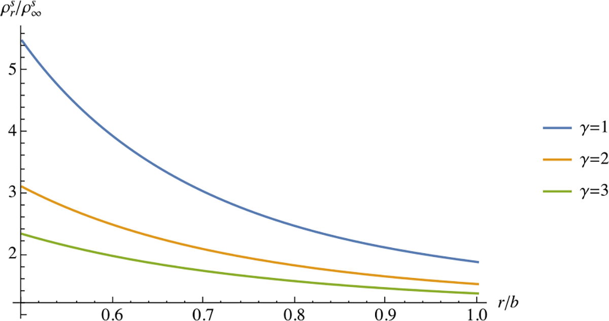
Steady-state response of ${\rho }_r^s/{\rho }_{\mathrm{\infty }}^s$ in Example 7, along the radius $r$ of a thick-walled cylindrical tube subjected to an internal pressure $p_0$. The inner wall radius is $a$ and the outer wall radius is $b$. Results are presented for $b/a=2$ and various values of $\gamma$

3. Mechanics of Constrained Mixtures

The equations of momentum balance for constrained mixture constituents were presented previously [9]. A notable finding from that earlier study is that the state of stress in individual mixture constituents remains indeterminate. This indeterminacy occurs because the internal forces resulting from momentum exchanges between constrained constituents remain unobservable due to lack of relative motion between them. The only observable stress measure is the mixture stress $\mathit{\sigma }$, which may be evaluated from the mixture momentum balance. Under quasi-static conditions, in the absence of external body forces, this equation reduces to the familiar relation

$$\mathrm{d}\mathrm{i}\mathrm{v}\mathit{\sigma }=0.$$ (3.1)

To solve for the function of state $\mathit{\sigma }$, it is necessary to first select the desired list of state variables for describing the response of biological tissues. Under isothermal processes, when analyzing reactive solid constituents in a constrained mixtures, we choose $(\theta ,{\mathbf{F}}^{\beta },{\rho }_r^{\beta })$ as our list of state variables, where $\beta$ spans all constituents $\alpha$ in the mixture [9]. The absolute temperature $\theta$ is included since material properties appearing in the constitutive relations for $\mathit{\sigma }$ and ${\hat{\rho }}^{\alpha }$, such as reaction rates, may vary with temperature. The deformation gradients ${\mathbf{F}}^{\beta }$ are included to account for the role of solid matrix strain. The referential apparent densities ${\rho }_r^{\beta }$ are included since they may evolve in time and space in reactive processes, thereby altering material properties over time.

Given these state variables, the axiom of entropy inequality imposes the following thermodynamic constraint on $\mathit{\sigma }$,

$$\sigma =\frac{1}{J^s}\sum _{\alpha }\frac{\partial {\Psi }_r}{\partial {\mathbf{F}}^{\alpha }}\cdot {\left({\mathbf{F}}^{\alpha }\right)}^T,$$ (3.2)

where ${\Psi }_r$ is the referential mixture free energy density, which may be evaluated from the specific free energy ${\psi }^{\alpha }$ of each constituent $\alpha$ according to

$${\Psi }_r=\sum _{\alpha }{\rho }_r^{\alpha }{\psi }^{\alpha }.$$ (3.3)

Other constraints imposed by the axiom of entropy inequality are $H_r=-\partial {\Psi }_r/\partial \theta$, where $H_r$ is the referential mixture entropy density, and $\mathbf{q}=0$, where $\mathbf{q}$ is the heat flux in the mixture, leaving the residual dissipation

$$\sum _{\alpha }{\hat{\rho }}^{\alpha }{\mu }^{\alpha }\le 0,$$ (3.4)

where

$${\mu }^{\alpha }=\frac{\partial {\Psi }_r}{\partial {\rho }_r^{\alpha }}$$ (3.5)

represents the chemical potential of constituent $\alpha$.

The residual dissipation effectively places a thermodynamic constraint on the constitutive relations for mass supplies ${\hat{\rho }}^{\alpha }$. When the inequality in (3.4) is violated, the reaction embodied in ${\hat{\rho }}^{\alpha }$ may not proceed. Students of chemistry may recognize this inequality constraint as equivalent to the requirement that chemical reactions may only proceed when they produce a net reduction in the Gibbs energy [55].²

In summary, the mixture momentum balance (3.1) and constituent mass balances (2.23) may be solved simultaneously for the unknowns ${\mathbf{F}}^s$ and ${\rho }_r^{\alpha }$, given constitutive relations for ${\Psi }_r$ and ${\hat{\rho }}^{\alpha }$, and constitutive assumptions for ${\mathbf{F}}^{\alpha s}$.

Example 8

Under infinitesimal strain analyses, the relation (3.2) for the mixture stress simplifies to

$$\sigma =\sum _{\alpha }\frac{\partial {\Psi }_r}{\partial {\epsilon }^{\alpha }}.$$ (3.6)

For example, assuming linear elasticity, the mixture strain energy density may be given by

$${\Psi }_r=\sum _{\alpha }\frac{1}{2}{\epsilon }^{\alpha }:{𝒞}^{\alpha }({\rho }_r^{\beta }):{\epsilon }^{\alpha },$$ (3.7)

where ${\mathbf{𝒞}}^{\alpha }({\rho }_r^{\beta })$ is the fourth-order elasticity tensor for constituent $\alpha$. In this example, to maintain some generality, we have assumed that the elasticity of constituent $\alpha$ may depend on the referential apparent density of all constituents $\beta$ in the mixture. Based on this relation, the mixture stress simplifies to

$$\sigma =\sum _{\alpha }{𝒞}^{\alpha }({\rho }_r^{\beta }):{\epsilon }^{\alpha }=\sum _{\alpha }𝒞({\rho }_r^{\beta }):({\epsilon }^s-{\epsilon }^{\alpha s}),$$ (3.8)

where we have used the general relation (2.11) between the strain tensor of constituent $\alpha$ relative to the master constituent $s$.

3.1. Non-reactive Elasticity

3.1.1. Tissues with Distinct Fiber Orientations

The simplest application of constrained mixtures of solid constituents is the classical field of non-reactive elasticity $\left({\hat{\rho }}^{\alpha }=0,\forall \alpha \right)$, when all constituents $\alpha$ share the same reference configuration ${\mathbf{X}}^s$. In that case, the mixture stress in (3.2) simplifies to

$$\mathit{\sigma }\left(\theta ,{\mathbf{F}}^s\right)=\frac{1}{J^s}\frac{\partial {\Psi }_r}{\partial {\mathbf{F}}^s}\cdot {\left({\mathbf{F}}^s\right)}^T.$$ (3.9)

Example 9

Consider a fibrous tissue consisting of multiple fiber bundles, initially oriented along distinct directions in the reference configuration. We may associate each bundle with a distinct constituent $\alpha$, so that the referential orientation of that bundle is given by the unit vector ${\mathbf{n}}_r^{\alpha }$; similarly, we can characterize that bundle’s mass content using ${\rho }_r^{\alpha }$ (which is time-invariant in this non-reactive example). For simplicity, we use infinitesimal strain theory and linear elasticity, though the same presentation may be given using finite deformation with nonlinear elasticity. Therefore, the stress response may be specialized from (3.8) with ${\mathit{\epsilon }}^{\alpha s}=0$, since all constituents share the same reference configuration,

$$\sigma =\sum _{\alpha }{𝒞}^{\alpha }:{\epsilon }^s.$$ (3.10)

The normal strain ${\epsilon }_n^{\alpha }$ in bundle $\alpha$ is given by ${\epsilon }_n^{\alpha }={\mathbf{n}}_r^{\alpha }\cdot {\mathit{\epsilon }}^s\cdot {\mathbf{n}}_r^{\alpha }$. Assuming that each fiber bundle behaves as a one-dimensional structure, and that its material properties only depend on its own density, the elasticity tensor may be expressed as

$${\mathbf{𝒞}}^{\alpha }=E\left({\rho }_r^{\alpha }\right){\mathbf{n}}_r^{\alpha }\otimes {\mathbf{n}}_r^{\alpha }\otimes {\mathbf{n}}_r^{\alpha }\otimes {\mathbf{n}}_r^{\alpha },$$ (3.11)

where $E\left({\rho }_r^{\alpha }\right)$ is Young’s modulus for fiber bundle $\alpha$. Combining these expressions, and further assuming that fiber bundles sustain stress only in tension, we get

$$\sigma =\sum _{\alpha }H\left({\epsilon }_n^{\alpha }\right)E\left({\rho }_r^{\alpha }\right){\epsilon }_n^{\alpha }{\mathbf{n}}_r^{\alpha }\otimes {\mathbf{n}}_r^{\alpha },$$ (3.12)

where $H(\cdot )$ is the Heaviside unit step function. This relation shows that the contribution of each fiber bundle to the mixture stress is weighted by the bundle’s modulus $E\left({\rho }_r^{\alpha }\right)$, which may generally be a nonlinear function of ${\rho }_r^{\alpha }$. This formulation is consistent with a fibrous cartilage model reported in an earlier study, without explicitly appealing to the concept of constrained mixtures [8]. In the case of a linear constitutive model, $E\left({\rho }_r^{\alpha }\right)=c{\rho }_r^{\alpha }$, where $c$ is a constant, we effectively propose that the weight factor of each fiber bundle is directly proportional to its mass content ${\rho }_r^{\alpha }$. Then, the expression (3.12) becomes consistent with the classical treatment of fibrous tissues consisting of multiple fiber bundles; it may be easily generalized to continuous fiber distributions by suitably substituting the summation with an integration over all directions ${\mathbf{n}}_r^{\alpha }$ [36, 37]. The densities ${\rho }_r^{\alpha }$ are observable (measurable) state variables. They may be directly related to the fiber angular distribution function $R\left({\mathbf{n}}_r^{\alpha }\right)$, which represents the fraction of total fibers oriented along ${\mathbf{n}}_r^{\alpha }$ in the reference configuration, and is routinely reported in the soft tissue mechanics literature [3, 23, 35, 45, 48].

Importantly, this example illustrates that the tissue ultrastructure can be directly related to its composition (mass content), since each constituent $\alpha$ represents a fiber bundle oriented in a different direction. More complex relations between ultrastructure and composition may be similarly formulated. For example, the ultrastructure of trabecular bone may be characterized by the concentrations ${\rho }_r^{\beta }$ of various critical sub-structures, such as rods and plates with particular dimensional characteristics, and their connectivities. Thus, the evolution of tissue ultrastructure during tissue remodeling may be entirely described by the axiom of mass balance, using scalar observable variables ${\rho }_r^{\beta }$.

3.1.2. Tissues with Distinct Fiber Reference Configurations

In our second example, consider multiple fiber bundles $\alpha$ which are all oriented along the same direction ${\mathbf{n}}_r$ in the master reference configuration. Each bundle $\alpha$ has a distinct reference configuration ${\mathbf{X}}^{\alpha }$, so that the relative strain tensors ${\mathit{\epsilon }}^{\alpha s}$, which are prescribed by constitutive assumption, are not zero. Assuming that the elasticity tensor has the same form as (3.11), with ${\mathbf{n}}_r^{\alpha }={\mathbf{n}}_r$ for all $\alpha$, and accounting for the tension-only response of fiber bundles, the stress-strain response of (3.8) may be rearranged as

$$\sigma =\sum _{\alpha }H\left({\epsilon }_n^s-{\epsilon }_n^{\alpha s}\right)E\left({\rho }_r^{\alpha }\right)\left({\epsilon }_n^s-{\epsilon }_n^{\alpha s}\right){\mathbf{n}}_r\otimes {\mathbf{n}}_r,$$ (3.13)

where ${\epsilon }_n^s={\mathbf{n}}_r\cdot {\mathit{\epsilon }}^s\cdot {\mathbf{n}}_r$, and similarly for ${\epsilon }_n^{\alpha s}$. Note that ${\epsilon }_n^{\alpha s}$ represents the value of ${\epsilon }_n^s$ when bundle $\alpha$ transitions between compression and tension. In this example, fiber bundles are incrementally recruited as the normal strain ${\epsilon }_n^s$ exceeds the threshold ${\epsilon }_n^{\alpha s}$ of each bundle $\alpha$ (Fig. 5). This incremental recruitment may thus produce the typical toe region observed in experimental measurements on fibrous tissues, as illustrated in the next example. The shape of the toe region may be modulated by the specific values of ${\epsilon }_n^{\alpha s}$ and the function $E\left({\rho }_r^{\alpha }\right)$ used for each bundle.

Fig. 5.

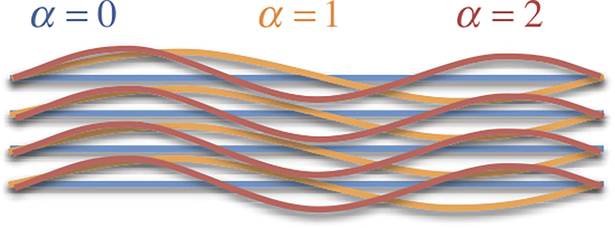
Schematic illustration of a constrained mixture of three fiber bundles $\alpha$, all oriented along the same direction ${\mathbf{n}}_r$, with distinct reference configurations. Each bundle is crimped by a different amount, such that the transition between compression and tension differs for each constituent $\alpha$. Let $\alpha =0$ correspond to the master constituent $s$, and let ${\epsilon }_n^s$ denote the normal strain along ${\mathbf{n}}_r$ in this bundle. We may define the relative normal strain ${\epsilon }_n^{\alpha s}$ along ${\mathbf{n}}_r$ as the value of ${\epsilon }_n^s$ at which bundle $\alpha$ transitions between compression and tension

Example 10

Consider a mixture of $n$ constituents ($\alpha =0$ to $n-1$, where $s$ corresponds to $\alpha =0)$ such that

$${\epsilon }^{\alpha s}=\frac{\alpha }{n}{\epsilon }_0,$$ (3.14a)

and

$$E\left({\rho }_r^{\alpha }\right)=\frac{E_0}{n}.$$ (3.14b)

Here, ${\epsilon }_0/n$ represents the uniform strain increment at which fiber bundles get consecutively recruited, whereas $E_0/n$ is the modulus of each fiber bundle.³ Under uniaxial loading along ${\mathbf{n}}_r$, with normal strain ${\epsilon }_n^s\equiv \epsilon$, we find that $\mathit{\sigma }=\sigma {\mathbf{n}}_r\otimes {\mathbf{n}}_r$ where

$$\sigma =\frac{E_0}{n}\sum _{\alpha =0}^{n-1}H\left(\epsilon -\frac{\alpha }{n}{\epsilon }_0\right)\left(\epsilon -\frac{\alpha }{n}{\epsilon }_0\right).$$ (3.14c)

A plot of $\sigma /E_0$ versus $\epsilon$ illustrates the fiber bundle recruitment within the toe region, and the linear response beyond it, for select values of $n$ (Fig. 6). This discrete fiber model may be generalized to a continuous fiber model $(n\to \mathrm{\infty })$ by converting the above summation to an integral,

$$\sigma =\frac{E_0}{{\epsilon }_0}{\int }_0^{{\epsilon }_0}H\left(\epsilon -\eta \right)\left(\epsilon -\eta \right)d\eta ,$$ (3.14d)

which produces

$$\sigma =E_0\left\{\begin{array}{ll}0& \epsilon <0\\ \frac{{\epsilon }^2}{2{\epsilon }_0}& 0\le \epsilon <{\epsilon }_0.\\ \epsilon -\frac{{\epsilon }_0}{2}& {\epsilon }_0\le \epsilon \end{array}\right.$$ (3.14e)

We conclude from this result that our specific constitutive assumptions for ${\epsilon }_n^{\alpha s}$ and $E\left({\rho }_r^{\alpha }\right)$ produce a quadratic toe region in the limit of a continuous fiber distribution, with ${\epsilon }_0$ representing the width of the toe region and $E_0$ representing the modulus of the linear region.

Fig. 6.

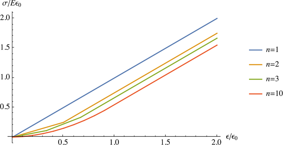
Stress-strain response for the fiber recruitment model described in Example 10, with increasing number of fiber bundles $n$ and uniform increment in recruitment strain

This modeling approach for progressive recruitment of fiber bundles has been used in many prior investigations [27, 32, 36, 67]; this example illustrates that this classical approach may be reproduced within the context of constrained, non-reactive mixtures. In the examples that follow, we illustrate how a reactive mixture framework easily extends these types of formulations to fibrous tissue growth and remodeling.

3.2. Reactive Elasticity

A reactive elasticity framework extends the previous examples by letting the apparent densities ${\rho }_r^{\alpha }$ evolve in response to various signals. In a biological tissue, cells may synthesize or degrade extracellular matrix in response to the state of loading. This type of response can be embodied in a suitable constitutive model for the mass supply ${\hat{\rho }}_r^{\alpha }$ for each constituent, which is then used in the mass balance equation (2.23). We have already illustrated this approach for a single solid constituent $s$ in Sect. 2.6.1. In the sections below we examine additional examples that illustrate common features in biological tissue growth and remodeling.

Example 11

We revisit the tissue model of Example 9, with distinct fiber orientations ${\mathbf{n}}_r^{\alpha }$, but common reference configuration ${\mathbf{X}}^s$. All fibers bundles start with a uniform density ${\rho }_r^{\alpha }={\rho }_0$ and lie in the $x_1-x_2$ plane, with bundle $\alpha$ oriented at an angle $\alpha$ from the $x_1$-axis (Fig. 7),

$${\mathbf{n}}_r^{\alpha }=\mathrm{c}\mathrm{o}\mathrm{s}\alpha {\mathbf{e}}_1+\sin \alpha {\mathbf{e}}_2.$$ (3.15a)

The fibrous matrix is initially isotropic in the $x_1-x_2$ plane. Consider that the tissue is now subjected to biaxial tension, such that the matrix of the stress $\mathit{\sigma }$ in the basis $\left\{{\mathbf{e}}_1,{\mathbf{e}}_2,{\mathbf{e}}_3\right\}$ is

$$[\mathit{\sigma }]=\left[\begin{array}{ccc}{\sigma }_1& 0& 0\\ 0& {\sigma }_2& 0\\ 0& 0& 0\end{array}\right],{\sigma }_1\ge {\sigma }_2\ge 0.$$ (3.15b)

Under infinitesimal strains the fiber bundle directions ${\mathbf{n}}_r^{\alpha }$ remain nearly unchanged, so that the normal stress along bundle $\alpha$ is

$$\sigma ={\mathbf{n}}_r^{\alpha }\cdot \mathit{\sigma }\cdot {\mathbf{n}}_r^{\alpha }={\sigma }_1{\mathrm{c}\mathrm{o}\mathrm{s}}^2\alpha +{\sigma }_2{\mathrm{s}\mathrm{i}\mathrm{n}}^2\alpha .$$ (3.15c)

We assume that the fibers remodel in response to loading according to the constitutive relation (2.38),

$$\frac{\partial {\rho }_r^{\alpha }}{\partial t}=B\left(\frac{{\Psi }_r^{\alpha }}{{\rho }_r^{\alpha }}-{\psi }_0^{\alpha }\right),{\Psi }_r^{\alpha }=\frac{{\sigma }^2}{2E\left({\rho }_r^{\alpha }\right)}.$$ (3.15d)

For simplicity, we assume a linear dependence of the fiber modulus $E\left({\rho }_r^{\alpha }\right)$ on referential apparent density,

$$E\left({\rho }_r^{\alpha }\right)=c{\rho }_r^{\alpha }.$$ (3.15e)

If we assume that ${\psi }_0^{\alpha }={\psi }_0$ is constant for all fibers, the steady-state remodeling response becomes

$${\rho }_{\mathrm{\infty }}^{\alpha }=\underset{t\to \mathrm{\infty }}{\mathrm{l}\mathrm{i}\mathrm{m}}{\rho }_r^{\alpha }={\rho }_{\mathrm{\infty }}\left({\mathrm{c}\mathrm{o}\mathrm{s}}^2\alpha +\frac{{\sigma }_2}{{\sigma }_1}{\mathrm{s}\mathrm{i}\mathrm{n}}^2\alpha \right),{\rho }_{\mathrm{\infty }}=\sqrt{\frac{{\sigma }_1^2}{2c{\psi }_0}}.$$ (3.15f)

If we assume that the fiber distribution is continuous, we may integrate the expression for ${\rho }_{\mathrm{\infty }}^{\alpha }$ in (f) with respect to $\alpha$ from 0 to $2\pi$ to get the mixture density,

$$\rho ={\rho }_{\mathrm{\infty }}\left(1+\frac{{\sigma }_2}{{\sigma }_1}\right)\pi .$$ (3.15g)

Then, the mass fraction of fibers along $\alpha$ may be evaluated from ${\rho }_{\mathrm{\infty }}^{\alpha }/\rho$. A plot of this fiber angular density distribution for various values of the ratio ${\sigma }_2/{\sigma }_1$ shows that fibers become preferentially denser in the direction of loading (Fig. 8). In the limiting case when ${\sigma }_2/{\sigma }_1=1$, the density distribution remains isotropic.

Fig. 7.

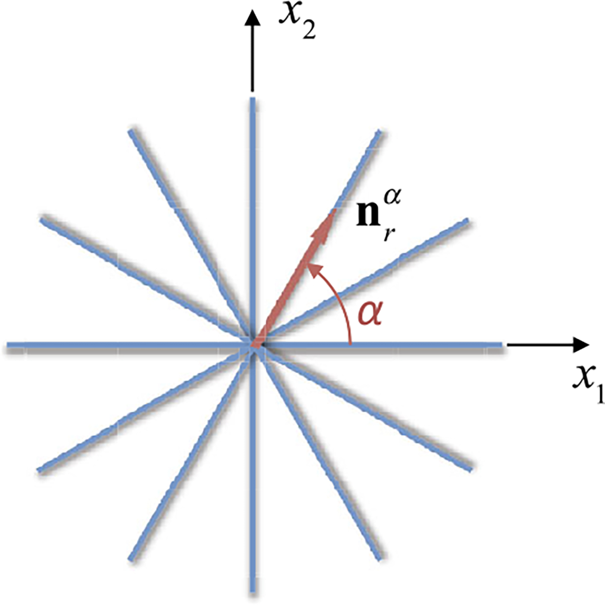
Planar fiber distribution in the $x_1-x_2$ plane. Constituent $\alpha$ in this constrained mixture represents the fiber bundle making an angle $\alpha$ with the $x_1$-axis

Fig. 8.

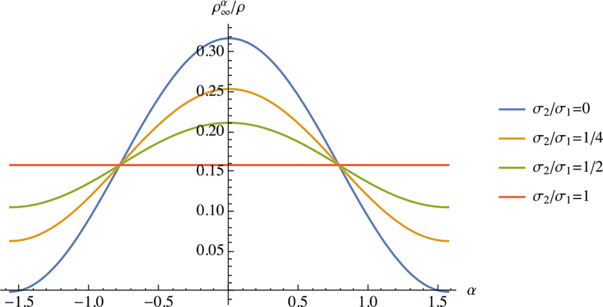
Steady-state remodeling response of fibers when ${\psi }_0^{\alpha }={\psi }_0$ is constant, as described in Example 11. Curves show the steady-state mass fraction ${\rho }_{\mathrm{\infty }}^{\alpha }/\rho$ of fiber bundles oriented at angle $\alpha$, for various values of the biaxial stress ratio ${\sigma }_2/{\sigma }_1$, as summarized in Eq. (3.15f)

Example 12

Alternatively, we may assume that the metabolic activity of cells is very sensitive to their orientation relative to the principal directions of stress. In that case, we may assume that the threshold value of the specific free energy ${\psi }_0^{\alpha }$ is nonlinearly dependent on the fiber orientation relative to the principal direction of stress,

$${\psi }_0^{\alpha }={\psi }_0{e}^{-2b\mathrm{c}\mathrm{o}\mathrm{s}2\alpha },b=\mathrm{l}\mathrm{n}\frac{{\sigma }_1}{{\sigma }_2}.$$ (3.16a)

In this model, the non-dimensional parameter $b$ controls the sensitivity of matrix remodeling to the ratio of principal stresses. The steady-state remodeling response of ${\rho }_r^{\alpha }$ under this state of stress is

$${\rho }_{\mathrm{\infty }}^{\alpha }=\underset{t\to \mathrm{\infty }}{\mathrm{l}\mathrm{i}\mathrm{m}}{\rho }_r^{\alpha }={\rho }_{\mathrm{\infty }}\left({\mathrm{c}\mathrm{o}\mathrm{s}}^2\alpha +e^{-b}{\mathrm{s}\mathrm{i}\mathrm{n}}^2\alpha \right)e^{b\mathrm{c}\mathrm{o}\mathrm{s}2\alpha },{\rho }_{\mathrm{\infty }}=\sqrt{\frac{{\sigma }_1^2}{2c{\psi }_0}}.$$ (3.16b)

For a continuous fiber distribution, integrating this expression over the range $0\le \alpha <2\pi$ produces the mixture density

$$\rho ={\rho }_{\mathrm{\infty }}\left[\left(1+e^{-b}\right)I_0(b)+\left(1-e^{-b}\right)I_1(b)\right]\pi ,$$ (3.16c)

where $I_0$ and $I_1$ are modified Bessel functions of the first kind, of order 0 and 1, respectively. A plot of ${\rho }_{\mathrm{\infty }}^{\alpha }/\rho$ versus $\alpha$, for various choices of $b$, shows that fibers are recruited preferentially along the dominant loading direction $(\alpha =0)$, with a fiber angular distribution that narrows considerably with increasing $b$ (Fig. 9). Once again, in the special case when ${\sigma }_2={\sigma }_1$ $(b=0)$, we note that the fiber angular distribution remains isotropic (${\rho }_{\mathrm{\infty }}^{\alpha }/\rho =1/2\pi$ for all $\alpha$). In contrast to the previous example, the remodeling response produces a much narrower fiber distribution for this choice of constitutive model for ${\psi }_0^{\alpha }$. In fact, the constitutive relation given in (3.16a) was selected specifically to reproduce the $\pi$-periodic von Mises fiber angular distribution, commonly used to model fibrous biological tissues [23, 48].

Fig. 9.

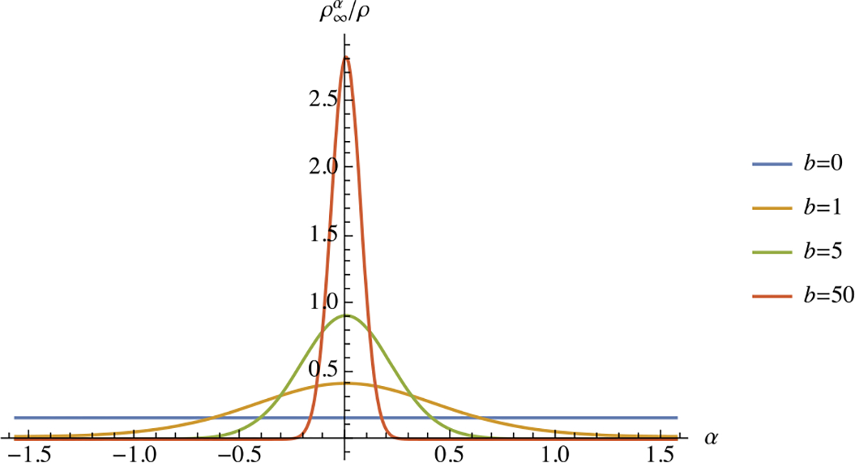
Steady-state remodeling response of fibers as described in Example 12, showing the mass fraction ${\rho }_{\mathrm{\infty }}^{\alpha }/{\rho }_{\mathrm{\infty }}$ of fiber bundles oriented along $\alpha$, for various values of the parameter $b$

3.3. Multi-generational Growth

When growth occurs in a biological tissue, the newly deposited solid material may not necessarily be in the same state of stress as the existing substrate. Therefore, we can treat each new generation of deposited solid material as a new constituent $\alpha$ within a constrained mixture, having its own distinct reference configuration ${\mathbf{X}}^{\alpha }$. The reference configuration of each generation becomes a constitutive assumption in the modeling of a growing tissue. A more comprehensive treatment of multi-generational growth mechanics has been presented previously [9].

A critical question that arises in this context is whether the newly deposited matrix should be in a stress-free state, or stressed. If it is stressed, should its state of stress match that of the underlying substrate or should it be distinct from it? The answer to any of these questions depends very much on the specifics of a given growth process, including environmental conditions at the time of matrix deposition, and the potential need to account for microscopic-level phenomena (such as molecular forces that stretch or coil a long-chain molecule as it binds to its substrate). For example, looking at Fig. 5, we need to hypothesize the manner by which cells synthesized fiber bundles at different time points, under different loading conditions, such that they were deposited within the extracellular matrix with different amounts of crimping.

One simple constitutive assumption is that the newly-deposited matrix is in the same state of strain as the underlying substrate, implying that ${\mathbf{X}}^{\alpha }={\mathbf{X}}^s,{\mathbf{F}}^{\alpha }={\mathbf{F}}^s$ and ${\mathbf{F}}^{\alpha s}=\mathbf{I}$ (or ${\mathit{\epsilon }}^{\alpha }={\mathit{\epsilon }}^s$ and ${\mathit{\epsilon }}^{\alpha s}=0$ under infinitesimal strains) for all generations $\alpha$. This assumption for multi-generational growth may be hard to justify physically, since it is difficult to explain how the newly-deposited matrix would bind onto the existing substrate while reproducing its current state of strain exactly. Therefore, we have to view that constitutive assumption as a simplifying idealization, satisfied approximately in an average sense, as might occur for example when the substrate is being loaded cyclically in tension and compression, while new material is continuously being added. In that case, the net macroscopic effect would be to produce a tissue with no apparent residual stresses, consistent with the idealization that the new matrix is being deposited in the same state of strain as the substrate. This type of growth is believed to occur in bone, since bone does not typically exhibit residual stresses, despite the fact that it remodels continually under load.

Another simple constitutive assumption is that the matrix of generation $\alpha$, newly deposited at time $t^{\alpha }$, is in a stress-free state, so that its reference configuration matches the current configuration of the tissue, ${\mathbf{X}}^{\alpha }={\mathit{\chi }}^s\left({\mathbf{X}}^s,t^{\alpha }\right)$. This assumption implies that ${\mathbf{F}}^{\alpha s}\left({\mathbf{X}}^s\right)={\mathbf{F}}^s\left({\mathbf{X}}^s,t^{\alpha }\right)$ (or ${\mathit{\epsilon }}^{\alpha s}\left({\mathbf{X}}^s\right)={\mathit{\epsilon }}^s\left({\mathbf{X}}^s,t^{\alpha }\right)$ under infinitesimal strains), producing ${\mathbf{F}}^{\alpha }\left({\mathbf{X}}^s,t^{\alpha }\right)=\mathbf{I}$ (equivalently, ${\mathit{\epsilon }}^{\alpha }\left({\mathbf{X}}^s,t^{\alpha }\right)=0$). This assumption is easier to understand physically, since matrix products released from a cell are initially in soluble form, especially if we ignore molecular forces or assume that their effects average out to produce a stress-free state at the time of binding. This modeling assumption may account for the evolution of residual stresses in a tissue, when consecutive generations are deposited in different stress-free configurations, because the current configuration of the underlying substrate varies over time. This type of growth is consistent with observations of residual stresses in many soft tissues, such as articular cartilage, intervertebral disc, or arterial wall.

Importantly, both of these constitutive assumptions lead to observable measures for ${\mathbf{F}}^{\alpha s}$, since these measures are based on the observable deformation ${\mathbf{F}}^s$ of the master constituent. Thus, observation of the kinematics, ${\mathbf{F}}^s\left({\mathbf{X}}^s,t\right)$, and composition ${\rho }_r^{\alpha }\left({\mathbf{X}}^s,t\right)$, provides a complete determination of the state variables, whereas constitutive relations for ${\Psi }_r\left(\theta ,{\mathbf{F}}^s,{\rho }_r^{\alpha }\right)$ and ${\hat{\rho }}_r^{\alpha }\left(\theta ,{\mathbf{F}}^s,{\rho }_r^{\alpha }\right)$, and constitutive assumptions for ${\mathbf{F}}^{\alpha s}$, provide the functions of state necessary for this framework.

Example 13

Consider uniaxial loading of a bar having a solid matrix whose first generation is the master constituent $s$. The prescribed uniaxial stress $\sigma \left(t\right)$ in the bar is given by

$$\sigma (t)=\left\{\begin{array}{ll}{\sigma }_0\frac{t}{t_0},& 0\le t<t_0,\\ {\sigma }_0,& t_0\le t<t_1,\\ {\sigma }_0\frac{t_2-t}{t_2-t_1},& t_1\le t\le t_2.\end{array}\right.$$ (3.17a)

This profile is illustrated in Fig. 10. We assume that a new generation $u$ is deposited interstitially, and homogeneously along the bar, over the time interval $t_0\le t<t_1$. The moduli of generations $s$ and $u$ are respectively $E^s=E\left({\rho }_r^s\right)$ and $E^u=E\left({\rho }_r^u\right)$, where $E$ is a given function of density. What is the history of the state of strain ${\epsilon }^s\left(t\right)$ ?

Fig. 10.

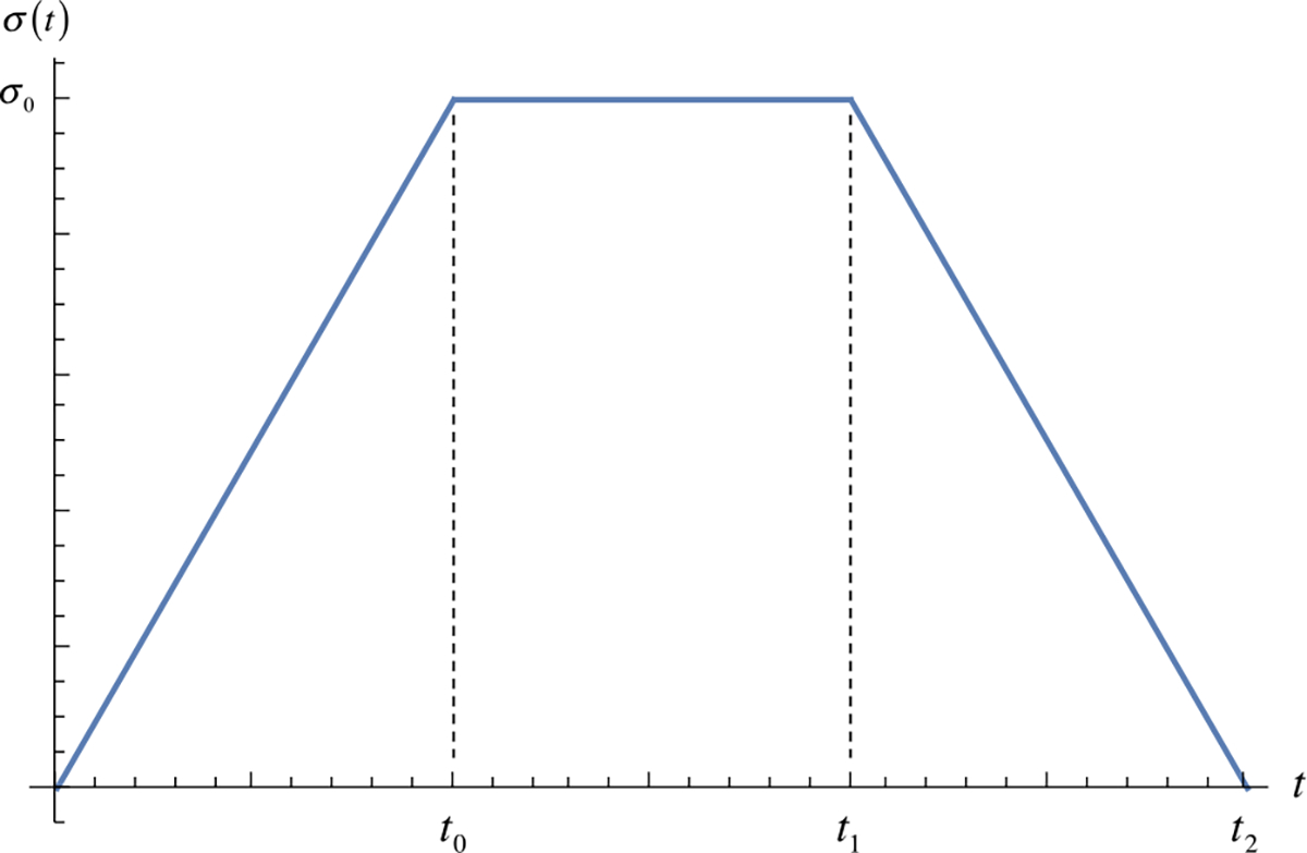
Prescribed uniaxial stress history $\sigma \left(t\right)$ for multi-generational growth problem in Example 13

We solve this problem using the infinitesimal strain relation (3.8), specialized to this one-dimensional analysis of a bar. The state of stress is already given, so our only challenge is to identify ${\epsilon }^{us}$ by constitutive assumption, and determine the history of ${\epsilon }^s$. We adopt the assumption that generation $u$ is deposited in a stress-free state over the time interval $t_0\le t<t_1$. The mixture stress may be evaluated from (3.8) as

$$\sigma \left(t\right)=\sum _{\alpha =s,u}E\left({\rho }_r^{\alpha }\right)\left({\epsilon }^s\left(t\right)-{\epsilon }^{\alpha s}\right)=\{\begin{array}{ll}{E}^s{\epsilon }^s\left(t\right),\hfill & 0\le t<t_0,\hfill \\ E^s{\epsilon }^s\left(t\right)+E\left({\rho }_r^u\right)\left({\epsilon }^s\left(t\right)-{\epsilon }^{us}\right),\hfill & t_0\le t<t_1,\hfill \\ E^s{\epsilon }^s\left(t\right)+E^u\left({\epsilon }^s\left(t\right)-{\epsilon }^{us}\right),\hfill & t_1\le t\le t_2.\hfill \end{array}$$ (3.17b)

Note that generation $u$ does not exist prior to $t=t_0$, therefore it does not contribute to the mixture stress prior to that time. Since generation $s$ does not grow or degrade, its density ${\rho }_r^s$ and its modulus $E^s$ are constants. The density ${\rho }_r^u$ of generation $u$ increases from 0 to its final value over the time interval $t_0\le t<t_1$, during which the modulus $E\left({\rho }_r^u\right)$ may evolve; however, from $t_1$ onward, the modulus $E^u=E\left({\rho }_r^u\right)$ remains constant. Equating (3.17a) and (3.17b) over the time interval $0\le t<t_0$, we can solve for ${\epsilon }^s\left(t\right)$ and conclude that

$${\epsilon }^{us}={\epsilon }^s\left(t_0\right)=\frac{{\sigma }_0}{E^s}.$$ (3.17c)

Substituting this relation into (3.17b) and equating the resulting expressions with corresponding time intervals in (3.17a), we obtain the complete history

$${\epsilon }^s\left(t\right)=\{\begin{array}{ll}\frac{{\sigma }_0}{E^s}\frac{t}{t_0},\hfill & 0\le t<t_0,\hfill \\ \frac{{\sigma }_0}{E^s},\hfill & t_0\le t<t_1,\hfill \\ \frac{{\sigma }_0}{E^s+E^u}(\frac{t_2-t}{t_2-t_1}+\frac{E^u}{E^s}),\hfill & t_1\le t\le t_2.\hfill \end{array}$$ (3.17d)

In particular, when the bar is unloaded at $t=t_2$, we find that the strain does not return to zero,

$${\epsilon }^s\left(t_2\right)=\frac{{\sigma }_0}{E^s+E^u}\frac{E^u}{E^s}.$$ (3.17e)

In other words, the bar does not return to the reference configuration of the master generation $s$, as the growth process has changed the traction-free configuration of the constrained mixture. The tissue has become stiffer due to the addition of mass in generation $u$. Because of the homogeneous growth and homogeneous state of stress throughout the growth history, the final state of stress is zero and the residual strain ${\epsilon }^s\left(t_2\right)$ is homogeneous along the entire length of the bar. Importantly, to an observer who only examines the bar starting at $t>t_2$, it is theoretically impossible to detect this residual strain because of its homogeneous distribution, nor is it possible to reconstruct the true growth history, regardless of the measurements performed. Thus, unobserved past growth history may only be hypothesized, but not fully reconstructed.

Since we are using linear infinitesimal strain theory, we can use the superposition principle as a quick way of reproducing the result of (3.17e). We recognize that the bar has a modulus of $E^e$ before growth, so that a stress ${\sigma }_0$ produces a strain ${\sigma }_0/E^e$. After growth, the bar’s modulus has increased to $E^s+E^u$, therefore a reversal of the prescribed stress, $-{\sigma }_0$, produces a strain $-{\sigma }_0/\left(E^s+E^u\right)$. Superposing these two prescribed stresses and resulting strains, the net stress becomes zero and the net strain is identical to the formula in (3.17e), as also illustrated in Fig. 11.

Fig. 11.

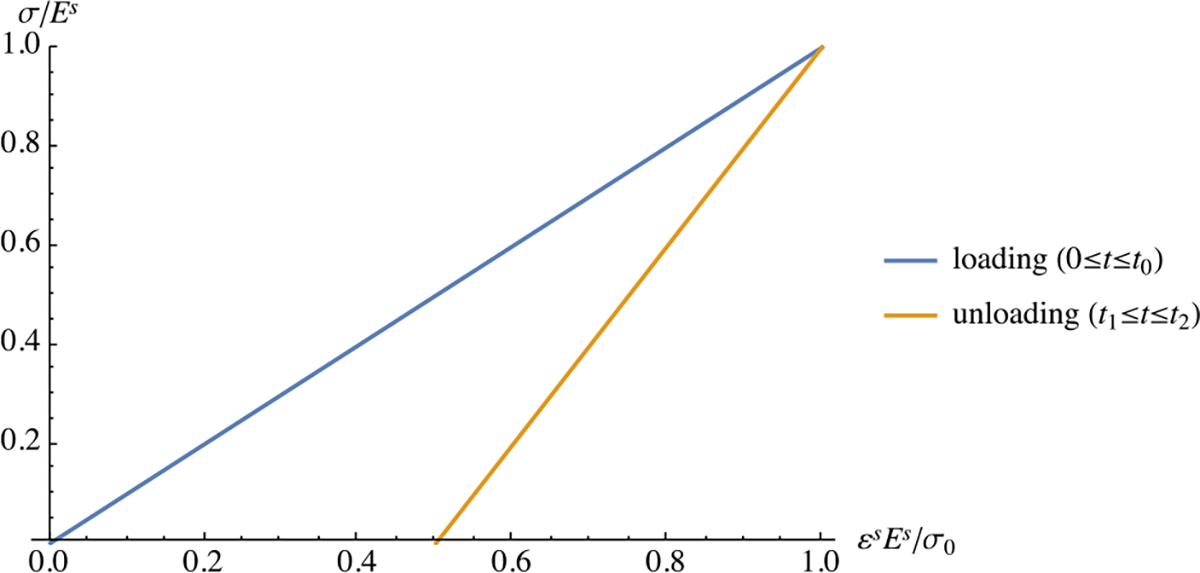
Stress-strain response for multigenerational growth of a uniaxially loaded bar. The response to loading of the first generation $\left(0\le t\le t_0\right)$ has a slope $E^s$. After the growth of the second generation from $t_0$ to $t_1$, the modulus has risen to $E^s+E^u$ and the unload from $t_1$ to $t_2$ produces a residual strain, as given by Eq. (3.17e) in Example 10. This illustration uses $E^u=E^s$

The above example illustrates homogeneous growth under a homogeneous state of stress, which produces homogeneous residual strain (but no residual stress) in the final, traction-free configuration of the constrained mixture. In the next example, we examine homogeneous interstitial growth (homogeneous deposition of ${\rho }_r^u$) under an inhomogeneous state of stress, using an internally pressurized thick-walled cylinder.

Example 14

Consider the thick-walled cylindrical tube analyzed in Example 7. Consider that the tube is subjected to an internal pressure $p\left(t\right)$. The resulting state of stress is given in that previous example. Consider that the pressure $p\left(t\right)$ varies over time according to

$$p(t)=\left\{\begin{array}{ll}{p}_0\frac{t}{t_0},& 0\le t<t_0,\\ p_0,& t_0\le t<t_1,\\ p_0\frac{t_2-t}{t_2-t_1},& t_1\le t\le t_2,\end{array}\right.$$ (3.18a)

and growth occurs over the time interval $t_0\le t<t_1$, in analogy to Example 13. Assuming that generations $s$ and $u$ behave as linear isotropic elastic materials with Poisson’s ratio equal to zero for both generations, what is the state of stress and strain in the traction-free state at $t=t_2$?

We solve this problem in the same manner as in Example 13, using the quick superposition method summarized at the end of that example. Based on the constitutive relation of a linear isotropic elastic solid, when Poisson’s ratio is zero, the non-zero normal strains of generation $s$ at time $t_0$ are given by

$$\begin{array}{rr}& {\epsilon }_{rr}^s\left(r,t_0\right)={\epsilon }_{rr}^{us}(r)=\frac{{\sigma }_{rr}}{E^s}=\frac{a^2}{b^2-a^2}\left(1-\frac{b^2}{r^2}\right)\frac{p_0}{E^s},\\ & {\epsilon }_{\theta \theta }^s\left(r,t_0\right)={\epsilon }_{\theta \theta }^{us}(r)=\frac{{\sigma }_{\theta \theta }}{E^s}=\frac{a^2}{b^2-a^2}\left(1+\frac{b^2}{r^2}\right)\frac{p_0}{E^s}.\end{array}$$ (3.18b)

After the growth of generation $u$, the modulus has increased to $E^s+E^u$. Therefore, the strains resulting from a negative internal pressure $-p_0$ have a similar form as (3.18b), with $p_0$ replaced by $-p_0$ and $E^s$ replaced by $E^s+E^u$. Superposing these two loading states produces a net state of strain at $t_2$ given by

$$\begin{array}{rr}& {\epsilon }_{rr}^s\left(r,t_2\right)=\frac{a^2}{b^2-a^2}\left(1-\frac{b^2}{r^2}\right)\frac{p_0}{E^s+E^u}\frac{E^u}{E^s},\\ & {\epsilon }_{\theta \theta }^s\left(r,t_2\right)=\frac{a^2}{b^2-a^2}\left(1+\frac{b^2}{r^2}\right)\frac{p_0}{E^s+E^u}\frac{E^u}{E^s}.\end{array}$$ (3.18c)

The state of stress at $t_2$ is evaluated from (3.8), using the stress-strain relation specialized to the case when Poisson’s ratio is zero, $\mathit{\sigma }=E\mathit{\epsilon }$, and we confirm that the stresses return to zero upon unloading, ${\sigma }_{rr}\left(r,t_2\right)={\sigma }_{\theta \theta }\left(r,t_2\right)=0$. The development of inhomogeneous residual strains, summarized in (3.18c) and plotted in Fig. 12, is a consequence of the multi-generational growth process under an inhomogeneous state of stress. Observing the material at time $t>t_2$ does not make it possible to reconstruct the growth history; however, the inhomogeneous strain state provides a hint that such a growth process has occurred. Cutting the tube radially at any location around its circumference will cause a deformation that breaks the axisymmetric geometry; this type of deformation serves as evidence that the tube was residually strained. After cutting, some residual stresses may develop in the tube.

Fig. 12.

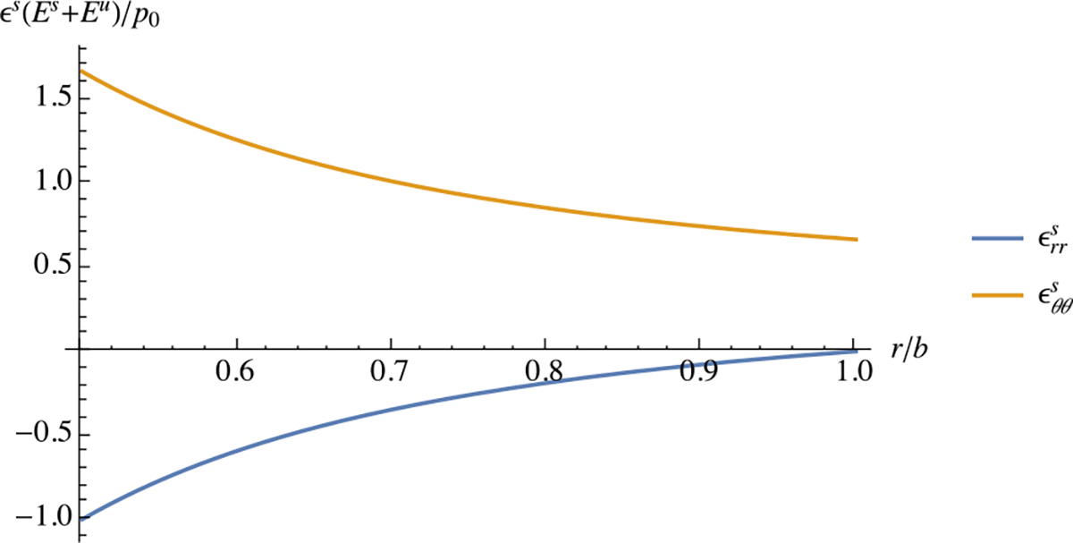
Residual radial and circumferential strains in multi-generational growth of a pressurized thick-walled cylindrical tube, as described in Example 14. In this example, $a=b/2$ and $E^u=E^s$

In conclusion, we find that a constrained reactive mixture framework allows us to account for tissue growth and remodeling, the evolution of fibrous tissue anisotropy in response to loading, and the evolution of residual strains and stresses. As shown in various examples, the tissue microstructure may be described entirely with compositional measures, namely, the concentrations ${\rho }_r^{\alpha }$ of various constituents, whose evolution is governed by the axiom of mass balance. No internal variables are needed to describe these processes, and this approach neatly recovers many classical formulations for biological tissues within a unified framework.

4. Reactive Linear Viscoelasticity

4.1. Strong and Weak Bonds

In this section we apply the framework of constrained reactive mixtures to formulate the theory of linear viscoelasticity for solids. A more comprehensive treatment of reactive nonlinear viscoelasticity has been presented in an earlier study [5]. Here, we treat viscoelastic solids as a mixture of two bond families: Strong bonds $(\alpha =e)$ that do not break in response to loading and produce the equilibrium elastic response; and weak bonds $\alpha \ne e$, which break in response to loading and immediately reform into a stress-free configuration. Weak bonds are therefore reactive constituents in this mixture framework. Weak bonds may belong to different bond families $b$ that exhibit different responses to loading; in this introductory presentation, we assume that a single weak bond family $b$ is present. This microscopic description of viscoelasticity was originally proposed by Green and Tobolsky [26] and this concept was reprized in more recent studies [64], though the present treatment differs from those prior articles.

Weak bonds that reform at time $t=u$ are denoted by $\alpha =u$ and called $u$-generation bonds. Similarly, weak bonds that break and reform at a subsequent time $t=v$ are denoted by $\alpha =v$. The reaction describing bond breaking and reforming is simply

$${ℰ}^u\to {ℰ}^v,$$ (4.1)

indicating that loaded bonds belonging to the $u$-generation break and reform into stress-free bonds at time $t=v$, forming $v$-generation bonds. The earliest generation is $\alpha =s$ where $s\to -\mathrm{\infty }$ and it represents the master constituent whose reference configuration is the stress-free configuration ${\mathbf{X}}^s$ of the weak bonds. We assume that ${\mathbf{X}}^s$ also represents the stress-free reference configuration of strong bonds. The motion of the master constituent is given by ${\mathit{\chi }}^s\left({\mathbf{X}}^s,t\right)$.

We adopt the constitutive assumption that bonds belonging to the $u$-generation have a stress-free reference configuration ${\mathbf{X}}^u$ that coincides with the current configuration at the time of bond reformation,

$${\mathbf{X}}^u={\mathit{\chi }}^s\left({\mathbf{X}}^s,u\right).$$ (4.2)

Based on the relation (2.11), the infinitesimal strain for this generation is

$${\mathit{\epsilon }}^u\left({\mathbf{X}}^s,t\right)={\mathit{\epsilon }}^s\left({\mathbf{X}}^s,t\right)-{\mathit{\epsilon }}^{us}\left({\mathbf{X}}^s\right).$$ (4.3)

This relation indicates that ${\mathit{\epsilon }}^u\left({\mathbf{X}}^s,t\right)$ is the strain relative to time $u$. The constitutive assumption of (4.2) implies that ${\mathit{\epsilon }}^{us}$ may be evaluated as

$${\mathit{\epsilon }}^{us}\left({\mathbf{X}}^s\right)={\mathit{\epsilon }}^s\left({\mathbf{X}}^s,u\right),$$ (4.4)

which remains invariant for all $t\ge u$. In other words, the strain ${\mathit{\epsilon }}^s$ of the master constituent uniquely determines the relative strain ${\mathit{\epsilon }}^u$ of all subsequent generations $u$.

4.2. Constitutive Model for Free Energy Density

We now propose a constitutive form for the mixture strain energy density ${\Psi }_r$,

$${\Psi }_r(\theta ,{\epsilon }^s,{\rho }_r^{\beta })={\Psi }_r^e\left(\theta ,{\epsilon }^s\right)+\sum _u{\Psi }_r^u\left(\theta ,{\rho }_r^u,{\epsilon }^u\right),$$ (4.5)

where ${\Psi }_r^e$ is the strain energy density of strong bonds and ${\Psi }_r^u$ is the strain energy density of $u$-generation bonds. The simplifying constitutive assumptions adopted here are that (a) ${\Psi }_r^e$ is independent of the weak bond concentrations, and (b) ${\Psi }_r^u$ only depends on the concentration ${\rho }_r^u$ of that generation. We make a further simplifying assumption that the free energy density of each generation has the same functional form for all generations,

$${\Psi }_r^u\left(\theta ,{\rho }_r^u,{\mathit{\epsilon }}^u\right)={\rho }_r^u{\psi }^b\left(\theta ,{\mathit{\epsilon }}^u\right),$$ (4.6)

where ${\psi }^b$ is the specific free energy of any generation in the bond family $b$, and is independent of the concentration of that generation. All these simplifications represent constitutive assumptions that may be validated against experimental measurements of specific viscoelastic solids.

Based on this constitutive model we find that the chemical potential of each bond generation, given by (3.5), reduces to

$${\mu }^u=\frac{\partial {\Psi }_r^u}{\partial {\rho }_r^u}={\psi }^b\left(\theta ,{\mathit{\epsilon }}^u\right),$$ (4.7)

which is the specific free energy of that bond. The chemical potential of strong bonds (which are non-reactive) is zero, ${\mu }^e=0$. The mixture stress may be evaluated by substituting (4.5) into (3.6),

$$\sigma =\frac{\partial {\Psi }_r^e}{\partial {\epsilon }^s}+\sum _u{\rho }_r^u\frac{\partial {\psi }^b\left(\theta ,{\epsilon }^u\right)}{\partial {\epsilon }^u}.$$ (4.8)

This relation may also be rewritten as $\mathit{\sigma }={\mathit{\sigma }}^e+{\mathit{\sigma }}^{\mathrm{v}}$, where

$${\mathit{\sigma }}^e=\frac{\partial {\Psi }_r^e}{\partial {\mathit{\epsilon }}^s}$$ (4.9)

is the elastic response of strong bonds, while

$${\sigma }^{\text{v}}=\sum _u{\rho }_r^u\frac{\partial {\psi }^b\left(\theta ,{\epsilon }^u\right)}{\partial {\epsilon }^u}$$ (4.10)

is the stress in weak bonds, which is effectively the viscous response since ${\rho }_r^u$ eventually decays to zero for all loaded bond generations, as shown below.

4.3. Constitutive Model for Mass Supply

The mass balance for each constituent of a constrained mixture is given in (2.23), subject to a suitable initial condition. Based on Sect. 2.4, the initial bond reaction ${ℰ}^s\to {ℰ}^u$ is constrained stoichiometrically by

$${\hat{\rho }}_r^u=-{\hat{\rho }}_r^s=M^s{\hat{\zeta }}_r,$$ (4.11)

where ${\hat{\zeta }}_r$ is the molar production rate and $M^s=M^u$ is the molar mass for this weak bond species. We now make the constitutive assumption that ${\hat{\zeta }}_r$ describes a first-order forward reaction, according to the law of mass action,

$$M^s{\hat{\zeta }}_r=\frac{1}{\tau }{\rho }_r^s,$$ (4.12)

where $1/\tau$ is the reaction rate and $\tau$ is the time constant of the reaction. Using a material frame to solve for ${\rho }_r^s\left({\mathbf{X}}^s,t\right)$, the mass balance for the $s$-generation becomes

$$\frac{\partial {\rho }_r^s}{\partial t}=-\frac{1}{\tau }{\rho }_r^s,$$ (4.13)

whose solution is

$${\rho }_r^s\left({\mathbf{X}}^s,t\right)={\rho }_0{e}^{-(t-u)/\tau },t\ge u.$$ (4.14)

Here, ${\rho }_0$ is the initial concentration of $s$-generation bonds of bond family $b$, which represents the total density of weak bonds in the mixture. The corresponding equation for ${\rho }_r^u$ is

$$\frac{\partial {\rho }_r^u}{\partial t}=\frac{1}{\tau }{\rho }_r^s=\frac{1}{\tau }{\rho }_0{e}^{-(t-u)/\tau },$$ (4.15)

with initial condition ${\rho }_r^u\left({\mathbf{X}}^s,u\right)=0$ at $t=u$. Therefore, the solution for ${\rho }_r^u$ is

$${\rho }_r^u\left({\mathbf{X}}^s,t\right)={\rho }_0\left(1-e^{-(t-u)/\tau }\right),t\ge u.$$ (4.16)

Next, consider the subsequent bond reaction ${ℰ}^u\to {ℰ}^v$, which starts at time $v$ and is assumed to exhibit the same reaction kinetics. Following the approach above, the governing equation for $u$-generation bonds is

$$\frac{\partial {\rho }_r^u}{\partial t}=-\frac{1}{\tau }{\rho }_r^u,$$ (4.17)

subject to the initial condition ${\rho }_r^u\left({\mathbf{X}}^s,v\right)={\rho }_0(1-e^{-(v-u)/\tau })$ obtained from (4.16). The solution to this equation is

$${\rho }_r^u\left({\mathbf{X}}^s,t\right)={\rho }_0\left(e^{-(t-v)/\tau }-e^{-(t-u)/\tau }\right),t\ge v.$$ (4.18)

Therefore,

$${\rho }_r^u\left({\mathbf{X}}^s,t\right)=\left\{\begin{array}{ll}0,& t<u,\\ {\rho }_0\left(1-e^{-(t-u)/\tau }\right),& u\le t<v,\\ {\rho }_0\left(e^{-(t-v)/\tau }-e^{-(t-u)/\tau }\right),& v\le t.\end{array}\right.$$ (4.19)

We may define the bond mass fraction

$$w^u\left({\mathbf{X}}^s,t\right)\equiv \frac{{\rho }_r^u\left({\mathbf{X}}^s,t\right)}{{\rho }_0},$$ (4.20)

such that $w^u$ is now given by

$$w^u\left({\mathbf{X}}^s,t\right)=\left\{\begin{array}{ll}0,& t<u,\\ 1-e^{-(t-u)/\tau },& u\le t<v,\\ e^{-(t-v)/\tau }-e^{-(t-u)/\tau },& v\le t\end{array}\right.$$ (4.21)

While $s$ - and $u$-generation bonds are breaking over time $t\ge v,v$-generation bonds are growing from the reformation of bonds from both prior generations, with ${\rho }_r^v$ satisfying

$$\frac{\partial {\rho }_r^v}{\partial t}=\frac{1}{\tau }\left({\rho }_r^s+{\rho }_r^u\right)=\frac{{\rho }_0}{\tau }{e}^{-(t-v)/\tau },$$ (4.22)

subject to ${\rho }_r^v\left({\mathbf{X}}^s,v\right)=0$. Thus, the solution for ${\rho }_r^v$ is

$${\rho }_r^v\left({\mathbf{X}}^s,t\right)={\rho }_0\left(1-e^{-(t-v)/\tau }\right),t\ge v,$$ (4.23)

such that $w^v={\rho }_r^v/{\rho }_0=1-e^{-(t-v)/\tau }$. Comparing this relation to (4.16), it becomes apparent that the relation for $w^u$ in (4.21) is recursive and applies to all subsequent generations (Fig. 13).

Fig. 13.

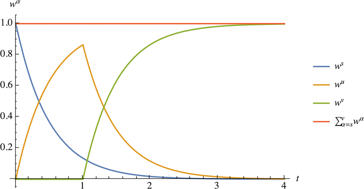
Temporal response of weak bond mass fractions $w^{\alpha }$ for three consecutive bond generations, where $\alpha$ denotes the time when that generation started forming: $s=-\mathrm{\infty },u=0,v=1$, with $\tau =1/2$. Based on the constraint of (2.24) and the definition (4.20), the bond mass fractions sum up to unity, ${\sum }_{\alpha }{w}^{\alpha }=1$

The mixture strain energy density and stress may be evaluated using these mass fractions as

$${\Psi }_r={\Psi }_r^e\left(\theta ,{\epsilon }^s\right)+\sum _u{w}^u{\Psi }_r^b\left(\theta ,{\epsilon }^u\right),$$ (4.24)

and

$$\sigma =\frac{\partial {\Psi }_r^e}{\partial {\epsilon }^s}+\sum _u{w}^u\frac{\partial {\Psi }_r^b\left(\theta ,{\epsilon }^u\right)}{\partial {\epsilon }^u},$$ (4.25)

where ${\Psi }_r^b\equiv {\rho }_0{\psi }^b$.

Example 15

The stress-relaxation response to a single step strain at $t=u$ may be evaluated from these expressions as follows. Let ${\mathit{\epsilon }}^s\left({\mathbf{X}}^s,t\right)=H(t-u){\mathit{\epsilon }}_0$. According to (4.4), we find that ${\mathit{\epsilon }}^{us}={\mathit{\epsilon }}_0$ so that ${\mathit{\epsilon }}^u\left({\mathbf{X}}^s,t\right)=0$ for $t\ge u$ according to (4.3). In other words, generation $u$ comes into existence at the instant of loading at $t=u$, and its reference configuration is the current configuration of the $s$-generation at $t=u$. Since ${\mathit{\epsilon }}^u\left({\mathbf{X}}^s,t\right)$ is zero, the $u$-generation strain energy density is equal to zero, ${\Psi }_r^b\left(\theta ,{\mathit{\epsilon }}^u\right)=0$. Therefore, the only contributions to the mixture strain energy density ${\Psi }_r$ are the strong bonds and the $s$-generation weak bonds, whose concentration is decaying over time according to (4.14),

$${\Psi }_r={\Psi }_r^e\left(\theta ,{\mathit{\epsilon }}_0\right)+e^{-(t-u)/\tau }{\Psi }_r^b\left(\theta ,{\mathit{\epsilon }}_0\right),t\ge u.$$ (4.26a)

Accordingly, at $t=u$, the strain energy density in the mixture is ${\Psi }_r={\Psi }_r^e\left(\theta ,{\mathit{\epsilon }}_0\right)+{\Psi }_r^b\left(\theta ,{\mathit{\epsilon }}_0\right)$, and as $t\to \mathrm{\infty }$, it decays to ${\Psi }_r={\Psi }_r^e\left(\theta ,{\mathit{\epsilon }}_0\right)$ (Fig. 14). Thus, instantaneously upon loading, both strong and weak bonds can store strain energy; however, the progressive breaking and reforming of weak bonds causes a concomitant dissipation of mixture strain energy density, eventually reducing to the contribution of strong bonds only. The stress response shows the identical behavior,

$$\mathit{\sigma }={\mathit{\sigma }}^e\left(\theta ,{\mathit{\epsilon }}_0\right)+e^{-(t-u)/\tau }{\mathit{\sigma }}^b\left(\theta ,{\mathit{\epsilon }}_0\right),t\ge u,$$ (4.26b)

where the strong and weak bond stresses are evaluated from their respective strain energy density functions as ${\mathit{\sigma }}^e=\partial {\Psi }_r^e/\partial \mathit{\epsilon }$ and ${\mathit{\sigma }}^b=\partial {\Psi }_r^b/\partial \mathit{\epsilon }$. Comparing the expression of (4.26b) to (4.8), we conclude that the viscous stress is ${\mathit{\sigma }}^{\mathrm{v}}=e^{-(t-u)/\tau }{\mathit{\sigma }}^b$. This example shows that the stress-strain response of strong and weak bonds need not be the same, since the constitutive relations for ${\Psi }_r^e$ and ${\Psi }_r^b$ may be different. In most classical, introductory presentations of linear viscoelasticity, it is common to select these functions to differ only by a scale factor. In particular, ${\Psi }_r^b=0$ produces an elastic solid; ${\Psi }_r^e=0$ produces a Maxwell fluid; and ${\Psi }_r^b=\beta {\Psi }_r^e$ produces the standard linear solid, where $\beta$ is a positive scalar.

Fig. 14.

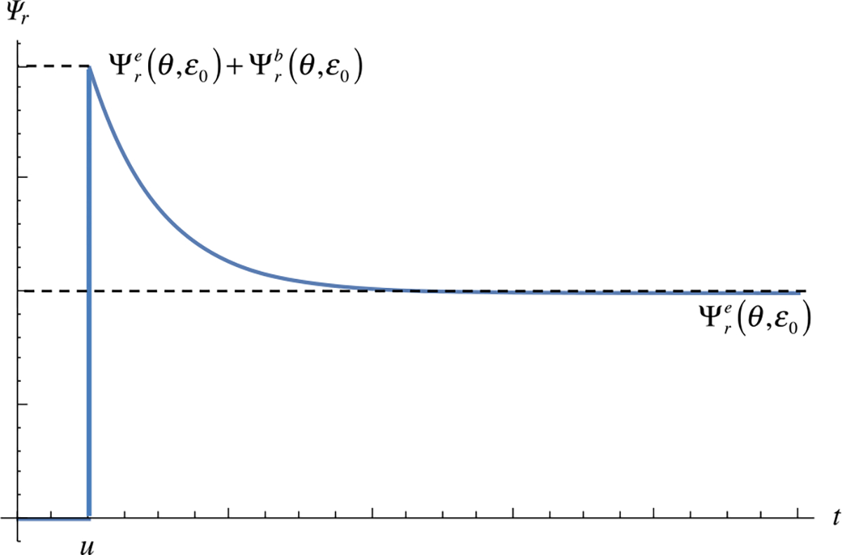
Time-dependent response of the free energy density ${\Psi }_r$ in a reactive viscoelastic material subjected to a step strain ${\mathit{\epsilon }}_0$ at time $t=u$, according to Example 15

For continuous time increments between consecutive generations, let $v=u+du$ in the recursive relation for $w^u$ in (4.21), and perform a Taylor series expansion of the third entry about $u$ to show that

$$w^u=\frac{1}{\tau }{e}^{-(t-u)/\tau }du,u\le t.$$ (4.27)

(The second entry in (4.21) reduces to zero as $v\to u$ and $t\to u$). Now, the summation in the evaluation of $\mathit{\sigma }$ may be converted to an integral,

$$\mathit{\sigma }=\frac{\partial {\Psi }_r^e}{\partial {\mathit{\epsilon }}^s}+{\int }_{-\mathrm{\infty }}^t\frac{1}{\tau }{e}^{-(t-u)/\tau }\frac{\partial {\Psi }_r^b\left(\theta ,{\mathit{\epsilon }}^u\right)}{\partial {\mathit{\epsilon }}^u}du.$$ (4.28)

We may define the function

$${\mathit{\sigma }}^b\left(\theta ,{\mathit{\epsilon }}^u\right)=\frac{\partial {\Psi }_r^b\left(\theta ,{\mathit{\epsilon }}^u\right)}{\partial {\mathit{\epsilon }}^u},$$ (4.29)

and use the definition of (4.9), so that the above expression for the stress may be rewritten as

$$\mathit{\sigma }={\mathit{\sigma }}^e\left(\theta ,{\mathit{\epsilon }}^s\right)+\frac{1}{\tau }{\int }_{-\mathrm{\infty }}^t{e}^{-(t-u)/\tau }{\mathit{\sigma }}^b\left(\theta ,{\mathit{\epsilon }}^u\right)du.$$ (4.30)

Similarly, the mixture free energy density is

$${\Psi }_r\left(\theta ,{\epsilon }^s,{\rho }_r^{\gamma }\right)={\Psi }_r^e\left(\theta ,{\epsilon }^s\right)+\sum _u{w}^u{\Psi }_r^b\left(\theta ,{\epsilon }^u\right)$$ (4.31)

in discrete form, and

$${\Psi }_r\left(\theta ,{\mathit{\epsilon }}^s,{\rho }_r^{\gamma }\right)={\Psi }_r^e\left(\theta ,{\mathit{\epsilon }}^s\right)+\frac{1}{\tau }{\int }_{-\mathrm{\infty }}^t{e}^{-(t-u)/\tau }{\Psi }_r^b\left(\theta ,{\mathit{\epsilon }}^u\right)du$$ (4.32)

in continuous form.

For a linear stress-strain relation for ${\mathit{\sigma }}^b$ versus ${\mathit{\epsilon }}^u$, the relation (4.3) between ${\mathit{\epsilon }}^u$ and ${\mathit{\epsilon }}^s$ implies that

$${\mathit{\sigma }}^b\left(\theta ,{\mathit{\epsilon }}^u\left({\mathbf{X}}^s,t\right)\right)={\mathit{\sigma }}^b\left(\theta ,{\mathit{\epsilon }}^s\left({\mathbf{X}}^s,t\right)\right)-{\mathit{\sigma }}^b\left({\mathit{\epsilon }}^s\left({\mathbf{X}}^s,u\right)\right).$$ (4.33)

This expression may be substituted into (4.30) to produce

$$\mathit{\sigma }={\mathit{\sigma }}^e\left({\mathit{\epsilon }}^s\left({\mathbf{X}}^s,t\right)\right)+{\mathit{\sigma }}^b\left({\mathit{\epsilon }}^s\left({\mathbf{X}}^s,t\right)\right)-\frac{1}{\tau }{\int }_{-\mathrm{\infty }}^t{e}^{-(t-u)/\tau }{\mathit{\sigma }}^b\left({\mathit{\epsilon }}^s\left({\mathbf{X}}^s,u\right)\right)du,$$ (4.34)

which is the classical relation for infinitesimal strain viscoelasticity in isotropic materials.

In summary, we were able to derive the theory of linear viscoelasticity without an ad hoc appeal to Boltzmann’s superposition principle. Similarly, we did not propose the existence of internal variables, such as the deformation of springs and dashpots placed in various parallel and series configurations, to produce the desired material response. Instead, we formulated a viscoelasticity theory based on the existence of microscopic weak bonds that break and reform in response to loading, which is the fundamental physical mechanism believed to describe viscoelasticity [26, 64]. This formulation shows that stress may be evaluated from the derivative of the strain energy density with respect to strain, as shown in (4.25) and (4.28), in analogy to elasticity theory.

Example 16

Consider the one-dimensional analysis of a bar subjected to uniaxial loading. Let the strong bond modulus be $E^e$ and the weak bond modulus be $E^b$, so that ${\sigma }^e=E^e{\epsilon }^s$ and ${\sigma }^b=E^b{\epsilon }^s$. Under a prescribed strain ${\epsilon }^s={\epsilon }_{0}H\left(t\right)$, the stress response is obtained from (4.34),

$$\sigma (t)=E^e{\epsilon }_{0}H(t)+E^b{\epsilon }_{0}H(t)-\frac{E^b{\epsilon }_0}{\tau }{\int }_0^t{e}^{-(t-u)/\tau }du,$$ (4.35a)

which evaluates to

$$\sigma (t)=E^e{\epsilon }_{0}H(t)\left(1+\frac{E^b}{E^e}{e}^{-t/\tau }\right).$$ (4.35b)

Thus, the stress relaxes exponentially from a peak value $\left(E^e+E^b\right){\epsilon }_0$ at $t=0$ to an equilibrium value $E^e{\epsilon }_0$ (Fig. 15).

Fig. 15.

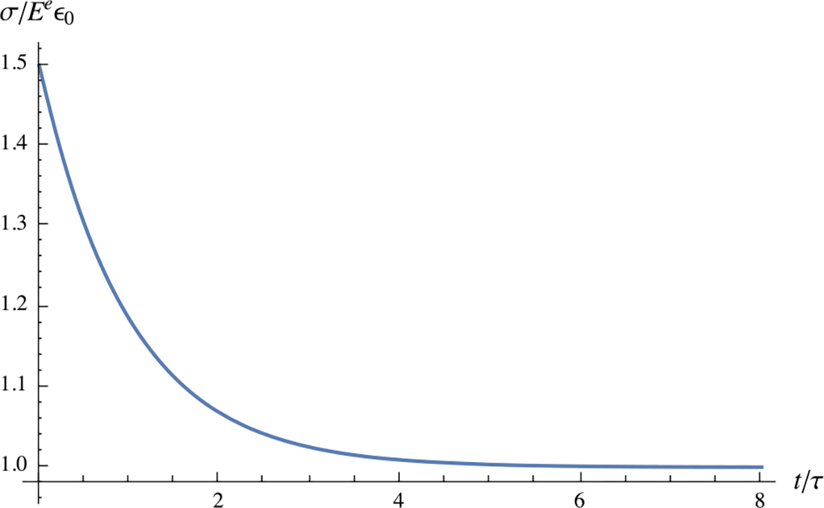
One-dimensional stress-relaxation response as described in Example 16, with $E^b/E^e=1/2$

Under a prescribed stress $\sigma ={\sigma }_{0}H\left(t\right)$, we solve for ${\epsilon }^s\left(t\right)$ using

$${\sigma }_{0}H(t)=\left(E^e+E^b\right){\epsilon }^s(t)-\frac{E^b}{\tau }{\int }_{-\mathrm{\infty }}^t{e}^{-(t-u)/\tau }{\epsilon }^s(u)du.$$ (4.35c)

This equation may be solved using the method of Laplace transforms to produce

$${\epsilon }^s(t)=\frac{{\sigma }_0}{E^e}\left(1-\beta e^{-\beta \frac{t}{\tau }}\right),\beta =\frac{E^b}{E^e+E^b}.$$ (4.35d)

This creep response shows that the strain is initially ${\sigma }_0/\left(E^e+E^b\right)$, and rises exponentially to an equilibrium value ${\sigma }_0/E^e$ (Fig. 16).

Fig. 16.

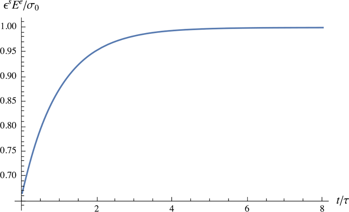
One-dimensional creep response as described in Example 16, with $E^b/E^e=1/2$

4.4. Thermodynamic Constraints

The reaction ${ℰ}^s\to {ℰ}^u$ involves two constituents and their referential mass supplies are given in (4.11), whereas the chemical potentials are given in (4.7). Substituting these relations into the residual dissipation (3.4) produces

$${\hat{\rho }}_r^s{\mu }^s+{\hat{\rho }}_r^u{\mu }^u=M^s{\hat{\zeta }}_r\left({\psi }^b\left(\theta ,{\mathit{\epsilon }}^u\right)-{\psi }^b\left(\theta ,{\mathit{\epsilon }}^s\right)\right)\le 0.$$ (4.36)

Note that $M^s{\hat{\zeta }}_r$ is always positive since the reaction proceeds forward (thus $\tau >0$), as seen from (4.12). We conclude that the thermodynamic constraint placed by the residual dissipation is that the specific free energy ${\psi }^b\left(\theta ,{\mathit{\epsilon }}^u\right)$ of broken and reformed bonds in the $u$-generation must be less than the specific free energy ${\psi }^b\left(\theta ,{\mathit{\epsilon }}^s\right)$ of intact bonds $s$. This constraint is automatically satisfied based on our modeling assumptions, since ${\mathit{\epsilon }}^u=0$ at time $u$, implying that ${\psi }^b\left(\theta ,{\mathit{\epsilon }}^u\right)=0$ at the time of $u$-generation bond reformation.

5. Conclusion

This article reviews some recent advances in modeling biological tissues using reactive constrained mixture theory. Many simple illustrations have been presented to highlight the potential benefits of this approach. The main message conveyed in this presentation is that seemingly disparate fields of mechanics and chemical kinetics are actually closely interrelated and may be elegantly expressed in a unified framework. Thus, constrained mixture models recover classical theories for fibrous materials with bundles oriented in different directions or having different reference configurations, that produce characteristic fiber recruitment patterns under loading. Reactions that exchange mass among various constituents of a mixture may be used to describe tissue growth and remodeling. Similarly, reactions that describe the breaking and reforming of bonds may be used to model free energy dissipation in a viscoelastic material.

In contrast to general (unconstrained) mixtures, constrained mixture only require the solution of a single momentum balance equation. No constitutive relations are needed to describe the momentum exchange among various constituents, since there is no relative motion between them within a constrained mixture framework. Therefore, just like elasticity theory, there is only one unknown motion ${\mathit{\chi }}^s\left({\mathbf{X}}^s,t\right)$ that needs to be obtained from the analysis of a constrained mixture, by solving the momentum balance for the mixture. When the mixture is reactive, the axiom of mass balance may be used to solve for the evolving concentration ${\rho }_r^{\alpha }\left({\mathbf{X}}^s,t\right)$ of mixture constituents $\alpha$. Much freedom exists in the formulation of constitutive relations for the mixture free energy density ${\Psi }_r\left(\theta ,{\mathbf{F}}^s,{\rho }_r^{\alpha }\right)$, constituent mass density supplies ${\hat{\rho }}_r^{\alpha }\left(\theta ,{\mathbf{F}}^s,{\rho }_r^{\alpha }\right)$, and constitutive assumptions about the mapping ${\mathbf{F}}^{\alpha s}$ between the reference configuration of constituent $\alpha$ and that of the master constituent $s$. Contrary to theories that employ internal variables, which necessarily evolve in time and require additional evolution equations [17], ${\mathbf{F}}^{\alpha s}$ is time-independent. It is a property of the mixture which is postulated by constitutive assumption when solid constituent $\alpha$ comes into existence. This approach allowed us to model the evolution of material anisotropy using ${\rho }_r^{\alpha }$ as the evolving measure of constituents with preferred spatial orientations, as illustrated with fibrous tissues in Sect. 3.2; a similar approach could be used with other quantitative measures of material structure, such as rods and plates in trabecular bone [62]. Importantly, the state variables $\left(\theta ,{\mathbf{F}}^s,{\rho }_r^{\alpha }\right)$ are all observable and governed by fundamental axioms of mass, momentum and energy balance, such that this framework does not require the introduction of additional evolution equations.

References

- 1.Armstrong CG: An analysis of the stresses in a thin layer of articular cartilage in a synovial joint. Eng. Med. 15(2), 55–61 (1986) [DOI] [PubMed] [Google Scholar]
- 2.Armstrong CG, Lai WM, Mow VC: An analysis of the unconfined compression of articular cartilage. J. Biomech. Eng. 106(2), 165–173 (1984) [DOI] [PubMed] [Google Scholar]
- 3.Aspden RM, Hukins DW: Collagen organization in articular cartilage, determined by X-ray diffraction, and its relationship to tissue function. Proc. R. Soc. Lond. B, Biol. Sci. 212(1188), 299–304 (1981) [DOI] [PubMed] [Google Scholar]
- 4.Ateshian GA: On the theory of reactive mixtures for modeling biological growth. Biomech. Model. Mechanobiol. 6(6), 423–445 (2007) [DOI] [PMC free article] [PubMed] [Google Scholar]
- 5.Ateshian GA: Viscoelasticity using reactive constrained solid mixtures. J. Biomech. 48(6), 941–947 (2015) [DOI] [PMC free article] [PubMed] [Google Scholar]
- 6.Ateshian GA, Ellis BJ, Weiss JA: Equivalence between short-time biphasic and incompressible elastic material responses. J. Biomech. Eng. 129(3), 405–412 (2007) [DOI] [PMC free article] [PubMed] [Google Scholar]
- 7.Ateshian GA, Morrison B III, Holmes JW, Hung CT: Mechanics of cell growth. Mech. Res. Commun. 42, 118–125 (2012) [DOI] [PMC free article] [PubMed] [Google Scholar]
- 8.Ateshian GA, Rajan V, Chahine NO, Canal CE, Hung CT: Modeling the matrix of articular cartilage using a continuous fiber angular distribution predicts many observed phenomena. J. Biomech. Eng. 131(6), 061003 (2009) [DOI] [PMC free article] [PubMed] [Google Scholar]
- 9.Ateshian GA, Ricken T: Multigenerational interstitial growth of biological tissues. Biomech. Model. Mechanobiol. 9(6), 689–702 (2010) [DOI] [PMC free article] [PubMed] [Google Scholar]
- 10.Azeloglu EU, Albro MB, Thimmappa VA, Ateshian GA, Costa KD: Heterogeneous transmural proteoglycan distribution provides a mechanism for regulating residual stresses in the aorta. Am. J. Physiol., Heart Circ. Physiol. 294(3), H1197–H1205 (2008) [DOI] [PubMed] [Google Scholar]
- 11.Bachrach NM, Mow VC, Guilak F: Incompressibility of the solid matrix of articular cartilage under high hydrostatic pressures. J. Biomech. 31(5), 445–451 (1998) [DOI] [PubMed] [Google Scholar]
- 12.Bedford A, Drumheller DS: Theories of immiscible and structured mixtures. Int. J. Eng. Sci. 21(8), 863–960 (1983) [Google Scholar]
- 13.Bowen RM: Thermochemistry of reacting materials. J. Chem. Phys. 49(4), 1625–1637 (1968) [Google Scholar]
- 14.Bryant MR, McDonnell PJ: A triphasic analysis of corneal swelling and hydration control. J. Biomech. Eng. 120(3), 370–381 (1998) [DOI] [PubMed] [Google Scholar]
- 15.Carter DR, Hayes WC: Bone compressive strength: the influence of density and strain rate. Science 194(4270), 1174–1176 (1976) [DOI] [PubMed] [Google Scholar]
- 16.Chahine NO, Wang CC-B, Hung CT, Ateshian GA: Anisotropic strain-dependent material properties of bovine articular cartilage in the transitional range from tension to compression. J. Biomech. 37(8), 1251–1261 (2004) [DOI] [PMC free article] [PubMed] [Google Scholar]
- 17.Coleman BD, Gurtin ME: Thermodynamics with internal state variables. J. Chem. Phys. 47(2), 597–613 (1967) [Google Scholar]
- 18.Cowin S, Hegedus D: Bone remodeling. I: Theory of adaptive elasticity. J. Elast. 6(3), 313–326 (1976) [Google Scholar]
- 19.Cyron CJ, Aydin RC, Humphrey JD: A homogenized constrained mixture (and mechanical analog) model for growth and remodeling of soft tissue. Biomech. Model. Mechanobiol. 15(6), 1389–1403 (2016) [DOI] [PMC free article] [PubMed] [Google Scholar]
- 20.Eberhardt AW, Keer LM, Lewis JL, Vithoontien V: An analytical model of joint contact. J. Biomech. Eng. 112(4), 407–413 (1990) [DOI] [PubMed] [Google Scholar]
- 21.Eringen AC, Ingram JD: A continuum theory of chemically reacting media—I. Int. J. Eng. Sci. 3(2), 197–212 (1965) [Google Scholar]
- 22.Fyhrie DP, Carter DR: A unifying principle relating stress to trabecular bone morphology. J. Orthop. Res. 4(3), 304–317 (1986) [DOI] [PubMed] [Google Scholar]
- 23.Gasser TC, Ogden RW, Holzapfel GA: Hyperelastic modelling of arterial layers with distributed collagen fibre orientations. J. R. Soc. Interface 3(6), 15–35 (2006) [DOI] [PMC free article] [PubMed] [Google Scholar]
- 24.Gleason RL, Humphrey JD: Effects of a sustained extension on arterial growth and remodeling: a theoretical study. J. Biomech. 38(6), 1255–1261 (2005) [DOI] [PubMed] [Google Scholar]
- 25.Gleason RL, Taber LA, Humphrey JD: A 2-d model of flow-induced alterations in the geometry, structure, and properties of carotid arteries. J. Biomech. Eng. 126(3), 371–381 (2004) [DOI] [PubMed] [Google Scholar]
- 26.Green M, Tobolsky A: A new approach to the theory of relaxing polymeric media. J. Chem. Phys. 14(2), 80–92 (1946) [Google Scholar]
- 27.Hill MR, Duan X, Gibson GA, Watkins S, Robertson AM: A theoretical and non-destructive experimental approach for direct inclusion of measured collagen orientation and recruitment into mechanical models of the artery wall. J. Biomech. 45(5), 762–771 (2012) [DOI] [PMC free article] [PubMed] [Google Scholar]
- 28.Hori RY, Mockros LF: Indentation tests of human articular cartilage. J. Biomech. 9(4), 259–268 (1976) [DOI] [PubMed] [Google Scholar]
- 29.Huiskes R, Weinans H, Grootenboer HJ, Dalstra M, Fudala B, Slooff TJ: Adaptive bone-remodeling theory applied to prosthetic-design analysis. J. Biomech. 20(11–12), 1135–1150 (1987) [DOI] [PubMed] [Google Scholar]
- 30.Humphrey J, Rajagopal K: A constrained mixture model for growth and remodeling of soft tissues. Math. Models Methods Appl. Sci. 12(03), 407–430 (2002) [Google Scholar]
- 31.Humphrey JD, Rajagopal KR: A constrained mixture model for arterial adaptations to a sustained step change in blood flow. Biomech. Model. Mechanobiol. 2(2), 109–126 (2003) [DOI] [PubMed] [Google Scholar]
- 32.Hurschler C, Loitz-Ramage B, Vanderby R Jr.: A structurally based stress-stretch relationship for tendon and ligament. J. Biomech. Eng. 119(4), 392–399 (1997) [DOI] [PubMed] [Google Scholar]
- 33.Karsaj I, Humphrey JD: A mathematical model of evolving mechanical properties of intraluminal thrombus. Biorheology 46(6), 509–527 (2009) [DOI] [PMC free article] [PubMed] [Google Scholar]
- 34.Kenyon DE: The theory of an incompressible solid-fluid mixture. Arch. Ration. Mech. Anal. 62(2), 131–147 (1976) [Google Scholar]
- 35.Lake SP, Miller KS, Elliott DM, Soslowsky LJ: Effect of fiber distribution and realignment on the nonlinear and inhomogeneous mechanical properties of human supraspinatus tendon under longitudinal tensile loading. J. Orthop. Res. 27(12), 1596–1602 (2009) [DOI] [PMC free article] [PubMed] [Google Scholar]
- 36.Lanir Y: A structural theory for the homogeneous biaxial stress-strain relationships in flat collagenous tissues. J. Biomech. 12(6), 423–436 (1979) [DOI] [PubMed] [Google Scholar]
- 37.Lanir Y: Constitutive equations for fibrous connective tissues. J. Biomech. 16(1), 1–12 (1983) [DOI] [PubMed] [Google Scholar]
- 38.Mak AF, Lai WM, Mow VC: Biphasic indentation of articular cartilage—I: Theoretical analysis. J. Biomech. 20(7), 703–714 (1987) [DOI] [PubMed] [Google Scholar]
- 39.Mansour JM, Mow VC: The permeability of articular cartilage under compressive strain and at high pressures. J. Bone Jt. Surg., Am. Vol. 58(4), 509–516 (1976) [PubMed] [Google Scholar]
- 40.Maroudas A, Bannon C: Measurement of swelling pressure in cartilage and comparison with the osmotic pressure of constituent proteoglycans. Biorheology 18(3–6), 619–632 (1981) [DOI] [PubMed] [Google Scholar]
- 41.Mow V, Kuei S, Lai W, Armstrong C: Biphasic creep and stress relaxation of articular cartilage in compression: theory and experiments. J. Biomech. Eng. 102(1), 73–84 (1980) [DOI] [PubMed] [Google Scholar]
- 42.Nims RJ, Durney KM, Cigan AD, Dusséaux A, Hung CT, Ateshian GA: Continuum theory of fibrous tissue damage mechanics using bond kinetics: application to cartilage tissue engineering. Interface Focus 6(1), 20150063 (2016) [DOI] [PMC free article] [PubMed] [Google Scholar]
- 43.Oloyede A, Broom ND: Is classical consolidation theory applicable to articular cartilage deformation? Clin. Biomech. 6(4), 206–212 (1991) [DOI] [PubMed] [Google Scholar]
- 44.Park S, Krishnan R, Nicoll SB, Ateshian GA: Cartilage interstitial fluid load support in unconfined compression. J. Biomech. 36(12), 1785–1796 (2003) [DOI] [PMC free article] [PubMed] [Google Scholar]
- 45.Pierce DM, Ricken T, Holzapfel GA: Modeling sample/patient-specific structural and diffusional responses of cartilage using dt-mri. Int. J. Numer. Methods Biomed. Eng. 29(8), 807–821 (2013) [DOI] [PubMed] [Google Scholar]
- 46.Prud’homme R: Flows of Reactive Fluids. Fluid Mechanics and Its Applications, vol. 94. Springer, New York: (2010) [Google Scholar]
- 47.Rachev A, Gleason RL Jr.: Theoretical study on the effects of pressure-induced remodeling on geometry and mechanical non-homogeneity of conduit arteries. Biomech. Model. Mechanobiol. 10(1), 79–93 (2011) [DOI] [PMC free article] [PubMed] [Google Scholar]
- 48.Sacks MS: Incorporation of experimentally-derived fiber orientation into a structural constitutive model for planar collagenous tissues. J. Biomech. Eng. 125(2), 280–287 (2003) [DOI] [PubMed] [Google Scholar]
- 49.Satha G, Lindström SB, Klarbring A: A goal function approach to remodeling of arteries uncovers mechanisms for growth instability. Biomech. Model. Mechanobiol. 13(6), 1243–1259 (2014) [DOI] [PMC free article] [PubMed] [Google Scholar]
- 50.Seyedsalehi S, Zhang L, Choi J, Baek S: Prior distributions of material parameters for Bayesian calibration of growth and remodeling computational model of abdominal aortic wall. J. Biomech. Eng. 137(10), 101001 (2015) [DOI] [PMC free article] [PubMed] [Google Scholar]
- 51.Soares JS, Sacks MS: A triphasic constrained mixture model of engineered tissue formation under in vitro dynamic mechanical conditioning. Biomech. Model. Mechanobiol. 15(2), 293–316 (2016) [DOI] [PMC free article] [PubMed] [Google Scholar]
- 52.Soltz MA, Ateshian GA: Experimental verification and theoretical prediction of cartilage interstitial fluid pressurization at an impermeable contact interface in confined compression. J. Biomech. 31(10), 927–934 (1998) [DOI] [PubMed] [Google Scholar]
- 53.Soltz MA, Ateshian GA: Interstitial fluid pressurization during confined compression cyclical loading of articular cartilage. Ann. Biomed. Eng. 28(2), 150–159 (2000) [DOI] [PubMed] [Google Scholar]
- 54.Timoshenko S, Goodier JN: Theory of Elasticity, 3rd edn. McGraw-Hill, New York: (1970) [Google Scholar]
- 55.Tinoco I, Sauer K, Wang JC: Physical Chemistry: Principles and Applications in Biological Sciences, 3rd edn. Prentice-Hall, Englewood Cliffs; (1995) [Google Scholar]
- 56.Torzilli P, Askari E, Jenkins J: Water content and solute diffusion properties in articular cartilage. In: Biomechanics of Diarthrodial Joints, vol. I, pp. 363–390. Springer, Berlin: (1990) [Google Scholar]
- 57.Urban JP, Maroudas A: Swelling of the intervertebral disc in vitro. Connect. Tissue Res. 9(1), 1–10 (1981) [DOI] [PubMed] [Google Scholar]
- 58.Valentín A, Holzapfel GA: Constrained mixture models as tools for testing competing hypotheses in arterial biomechanics: a brief survey. Mech. Res. Commun. 42, 126–133 (2012) [DOI] [PMC free article] [PubMed] [Google Scholar]
- 59.Vernerey FJ, Farsad M: A constrained mixture approach to mechano-sensing and force generation in contractile cells. J. Mech. Behav. Biomed. Mater. 4(8), 1683–1699 (2011) [DOI] [PubMed] [Google Scholar]
- 60.Wagenseil JE: A constrained mixture model for developing mouse aorta. Biomech. Model. Mechanobiol. 10(5), 671–687 (2011) [DOI] [PMC free article] [PubMed] [Google Scholar]
- 61.Wan W, Hansen L, Gleason RL Jr.: A 3-d constrained mixture model for mechanically mediated vascular growth and remodeling. Biomech. Model. Mechanobiol. 9(4), 403–419 (2010) [DOI] [PMC free article] [PubMed] [Google Scholar]
- 62.Wang J, Zhou B, Liu XS, Fields AJ, Sanyal A, Shi X, Adams M, Keaveny TM, Guo XE: Trabecular plates and rods determine elastic modulus and yield strength of human trabecular bone. Bone 72, 71–80 (2015) [DOI] [PMC free article] [PubMed] [Google Scholar]
- 63.Weinans H, Huiskes R, Grootenboer HJ: The behavior of adaptive bone-remodeling simulation models. J. Biomech. 25(12), 1425–1441 (1992) [DOI] [PubMed] [Google Scholar]
- 64.Wineman A: On the mechanics of elastomers undergoing scission and cross-linking. Int. J. Adv. Eng. Sci. Appl. Math. 1(2–3), 123–131 (2009) [Google Scholar]
- 65.Wong M, Ponticiello M, Kovanen V, Jurvelin JS: Volumetric changes of articular cartilage during stress relaxation in unconfined compression. J. Biomech. 33(9), 1049–1054 (2000) [DOI] [PubMed] [Google Scholar]
- 66.Wu J, Shadden SC: Stability analysis of a continuum-based constrained mixture model for vascular growth and remodeling. Biomech. Model. Mechanobiol. 15(6), 1669–1684 (2016) [DOI] [PubMed] [Google Scholar]
- 67.Zeinali-Davarani S, Wang Y, Chow M-J, Turcotte R, Zhang Y: Contribution of collagen fiber undulation to regional biomechanical properties along porcine thoracic aorta. J. Biomech. Eng. 137(5), 051001 (2015) [DOI] [PMC free article] [PubMed] [Google Scholar]