Mantis: A Fast, Small, and Exact Large-Scale Sequence-Search Index

SUMMARY

Sequence-level searches on large collections of RNA sequencing experiments, such as the NCBI Sequence Read Archive (SRA), would enable one to ask many questions about the expression or variation of a given transcript in a population. Existing approaches, such as the sequence Bloom tree, suffer from fundamental limitations of the Bloom filter, resulting in slow build and query times, less-than-optimal space usage, and potentially large numbers of false-positives. This paper introduces Mantis, a space-efficient system that uses new data structures to index thousands of raw-read experiments and facilitates large-scale sequence searches. In our evaluation, index construction with Mantis is 6× faster and yields a 20% smaller index than the state-of-the-art split sequence Bloom tree (SSBT). For queries, Mantis is 6–108× faster than SSBT and has no false-positives or -negatives. For example, Mantis was able to search for all 200,400 known human transcripts in an index of 2,652 RNA sequencing experiments in 82 min; SSBT took close to 4 days.

Graphical Abstract

In Brief

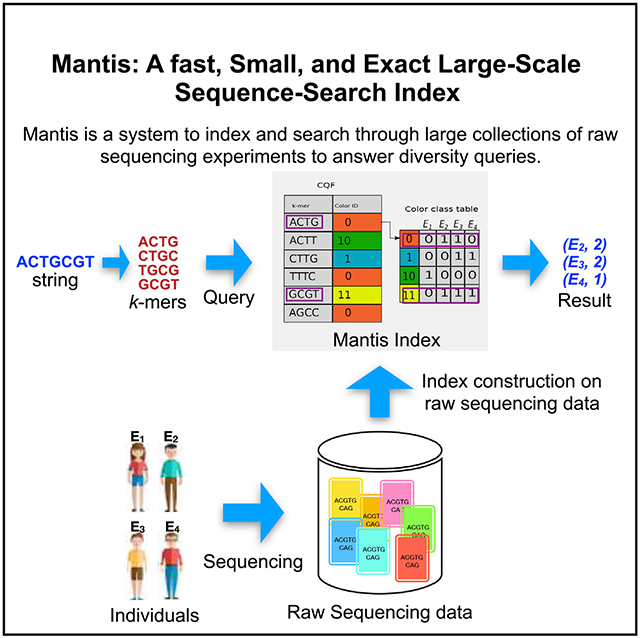
Mantis is a system to index and search through large collections of raw sequencing data. The query sequence can be a known or newly assembled gene or any valid nucleotide sequence. Mantis is faster and smaller than existing sequence-search tools and is exact in the sense that it does not report false-positives. To construct the index, Mantis indexes the k-mers (substrings of size k) in the reads of an experiment and then groups k-mers across experiments that exhibit the same patterns of occurrence.

INTRODUCTION

The ability to issue sequence-level searches over publicly available databases of assembled genomes and known proteins has played an instrumental role in many studies in the field of genomics, and has made BLAST (Altschul et al., 1990) and its variants some of the most widely used tools in all of science. Much subsequent work has focused on how to extend tools such as BLAST to be faster, more sensitive, or both (Buchfink et al., 2015; Daniels et al., 2013; Remmert et al., 2012; Steinegger and Söding, 2017). However, the strategies applied by such tools focus on the case where queries are issued over a database of reference sequences. However, the vast majority of publicly available sequencing data (e.g., the data deposited in the Sequence Read Archive [SRA]; Kodama et al., 2011) exist in the form of raw, unassembled sequencing reads. As such, these data have mostly been rendered impervious to sequence-level search, which substantially reduces the utility of such publicly available data.

There are a number of reasons that typical reference-database-based search techniques cannot easily be applied in the context of searching raw, unassembled sequences. One major reason is that most current techniques do not scale well as the amount of data grows to the size of the SRA (which today is ≈4 petabases of sequence information). A second reason is that searching unassembled sequences means that relatively long queries (e.g., genes) are unlikely to be present in their entirety as an approximate substring of the input.

Recently, new computational schemes have been proposed that hold the potential to allow searching raw SARs while overcoming these challenges. Solomon and Kingsford (2016) introduced the sequence bloom tree (SBT) data structure and an associated algorithm that enables an efficient type of search over thousands of sequencing experiments. Specifically, they re-phrase the query in terms of k-mer set membership in a way that is robust to the fact that the target sequences have not been assembled. The resulting problem is coined as the experiment discovery problem, where the goal is to return all experiments that contain at least some user-defined $\theta$ fraction of the k-mers present in the query string. The space and query time of the SBT structure has been further improved by Solomon and Kingsford (2017) and Sun et al. (2017) by applying an All-Some set decomposition over the original sets of the SBT structure. This seminal work introduced both a formulation of this problem and the initial steps toward a solution.

SBTs build on prior work using Bloom filters Bloom (1970). A Bloom filter is a compact representation of a set S. Bloom filters support insertions and membership queries, and they save space by allowing a small but tunable false-positive probability. That is, a query for an element $x\notin S$ might return “present” with probability $\delta$. Allowing false-positives enables the Bloom filter to save space; a Bloom filter can represent a set of size $n$ with a false-positive probability of $\delta$ using $O\left(n{\log }_2\left(\frac{1}{\delta }\right)\right)$ bits. Bloom filters have an interesting property that the bitwise-or of two Bloom filters representing ${\mathsf{S}}_1$ and ${\mathsf{S}}_2$ yields a Bloom filter for $S_1\cup S_2$. However, the false-positive rate of the union may increase substantially above $\delta$.

In k-mer-counting tools, Bloom filters are used to filter out single-occurrence (and likely erroneous) k-mers from raw-read data (Melsted and Pritchard, 2011). In a high-coverage genomic dataset, any k-mer that occurs only once is almost certainly an error and can thus be ignored. However, such k-mers can constitute a large fraction of all the k-mers in the input (typically 30%–50%) so allocating a counter and an entry in a hash table for these k-mers can waste a lot of space. Tools such as BFCounter (Melsted and Pritchard, 2011) and Jellyfish (Marçais and Kingsford, 2011) save space by inserting each k-mer into a Bloom filter the first time it is seen. For each k-mer in the input, the tool first checks whether the k-mer is in the Bloom filter. If not, then this is the first time this k-mer has been seen, so it is inserted into the filter. If the k-mer is already in the filter, then the counting tool stores the k-mer in a standard hash table, along with a count of the number of times this k-mer has been seen. In this application, a false-positive in the Bloom filter simply means that the tool might count a few k-mers that occur only once. Using Bloom filters in this way can reduce space consumption by roughly 50%.

SBTs use Bloom filters to index large sets of raw sequencing data probabilistically. In an SBT, each experiment is represented by a Bloom filter of all the k-mers that occur a sufficient number of times in that experiment. A k-mer counter can create such a Bloom filter by first counting all the k-mers in the experiment and then inserting every k-mer that occurs sufficiently often into a Bloom filter. The SBT then builds a binary tree by logically or-ing Bloom filters until it reaches a single root node. To find all the experiments that contain a k-mer x, the query procedure starts from the root and tests whether x is in the Bloom filter of each of the root’s children. Whenever a Bloom filter indicates that an element might be present in a subtree, the search procedure recurses into that subtree. Since Bloom filters do not admit false-negatives, k-mer absence from a filter allows early termination of the search procedure.

SBTs support queries for entire transcripts as follows. First compute the set $Q$ of k-mers that occur in the transcript. Then, when descending down the tree, only descend into subtrees whose root Bloom filter contains at least a fraction $\theta$ of the k-mers in $Q$. Typical values for $\theta$ proposed by Solomon and Kingsford (2016) are in the range 0.7–0.9. That is, any experiment that contains 70%–90% of the k-mers in $Q$ has a reasonable probability of containing the transcript (or a closely related variant).

The SSBT and the All-Some SBT have a similar structure to the SBT, but they use more efficient encodings. The All-Some SBT has a shorter construction time and query time than the SBT. The SSBT has a slower construction time than the SBT, answers queries faster than the SBT, and uses less space than either the SBT or the All-Some SBT.

Both structures use a similar high-level approach for saving space and thus making queries fast. Namely, instead of retaining a single Bloom filter at each internal node, the structures maintain two Bloom filters. One Bloom filter stores k-mers that appear in every experiment in the descendant leaves. These k-mers do not need to be stored in any descendants of the node, thus reducing the space consumption by reducing redundancy. If a queried k-mer is found in this Bloom filter, then it is known to be present in all descendant experiments. If the required fraction of k-mers for a search (i.e., $\theta$) ever appear in such a filter, then search of this subtree can terminate early as all descendant leaf nodes satisfy the query requirements. The other Bloom filter stores the rest of the k-mers, those that appear in some, but not all, of the descendants. All-Some SBT saves additional space by clustering similar leaves into subtrees so that more k-mers can be stored higher up in the tree and with less duplication.

Due to limitations of the Bloom filter, all of these SBT-like structures are forced to balance between the false-positive rate at the root and the size of the filters representing the individual experiments. Because Bloom filters cannot be resized, they must be created with enough space to hold the maximum number of elements that might be inserted. Furthermore, two Bloom filters can only be logically or-ed if they have the same size (and use the same underlying hash functions). Thus, the Bloom filters at the root of the tree must be large enough to represent every k-mer in every experiment indexed in the entire tree, while still maintaining a good false-positive rate. On the other hand, the Bloom filters at the leaves of the tree represent only a relatively small amount of data and, since there are many leaves, should be as small as possible.

Further complicating the selection of Bloom filter size is that individual dataset sizes vary by orders of magnitude, but all datasets must be summarized using Bloom filters of the same size. For these reasons, most of the Bloom filters in the SBT are, of necessity, sub-optimally tuned and inefficient in their use of space. SBTs partially mitigate this issue by compressing their Bloom filters using an off-the-shelf compressor (Bloom filters that are too large are sparse bit vectors and compress well). Nonetheless, SBTs are typically constructed with a Bloom filter size that is too small for the largest experiments and for the root of the tree. As a result, they have low precision: typically, only about 57%–67% of the results returned by a query are actually valid (i.e., contain at least a fraction $\theta$ of the query k-mers).

We present a new k-mer-indexing approach, which we call Mantis, that overcomes these obstacles. Mantis has several advantages over prior work:

• Mantis is exact. A query for a set $Q$ of k-mers and threshold $\theta$ returns exactly those datasets containing at least $\theta$ fraction of the k-mers in $\mathsf{Q}$. There are no false-positives or false-negatives. In contrast, we show that SBT-based systems exhibit only 57%–67% precision, meaning that many of the results returned for a given query are, in fact, false-positives.

• Mantis supports much faster queries than existing SBT-based systems. In our experiments, queries in Mantis ran up to 100× faster than in SSBT.

• Mantis supports much faster index construction. For example, we were able to build the Mantis index on 2,652 datasets in 16 hr. SSBT reported 97 hr to construct an index on the same collection of datasets.

• Mantis uses less storage than SBT-based systems. For example, the Mantis index for the 2,652 experiments used in the SSBT evaluation is 20% smaller than the compressed SSBT index for the same data.

• Mantis returns, for each experiment containing at least 1 k-mer from the query, the number of query k-mers present in this experiment. Thus, the full spectrum of relevant experiments can be analyzed. While these results can be post-processed to filter out those not satisfying a $\theta$ query, we believe the Mantis output is more useful, since one can analyze which experiments were close to achieving the $\theta$ threshold, and can examine if there is a natural “cutoff” at which to filter experiments.

Mantis (overview in Figure 1) builds on Squeakr (Pandey et al., 2017c), a k-mer counter based on the counting quotient filter (CQF) Pandey et al. (2017b). The CQF is a Bloom filter alternative that offers several advantages over the Bloom filter. First, the CQF supports counting; i.e., queries to the CQF return not only “present” or “absent” but also an estimate on the number of times the queried item has been inserted. Analogous to the Bloom filter’s false-positive rate, there is a tunable probability that the CQF may return a count that is higher than the true count for a queried element. CQFs can also be resized, and CQFs of different sizes can be merged together efficiently. Finally, CQFs can be used in an “exact” mode where they act as a compact exact hash table; i.e., we can make $\delta =0$. CQFs are also faster and more space efficient than Bloom filters for all practical configurations (i.e., any false-positive rate <1/64).

Figure 1. The Mantis Indexing Data Structures.

The CQF contains mappings from k-mers to color-class IDs. The color-class table contains mappings from color-class IDs to bit vectors. Each bit vector is N bits, where N is the number of experiments from which k-mers are extracted. The CQF is constructed by merging N input CQFs each corresponding to an experiment. A query first looks up the k-mer(s) in the CQF and then retrieves the corresponding color-class bit vectors from the color-class table.

Prior work has shown how CQFs can be used to improve performance and simplify the design of k-mer-counting tools (Pandey et al., 2017c) and de Bruijn graph representations (Pandey et al., 2017a). For example, Squeakr is essentially a thin wrapper around a CQF; it just parses fastq files, extracts the k-mers, and inserts them into a CQF. Other k-mer counters use multiple data structures (e.g., Bloom filters plus hash tables) and often contain sophisticated domain-specific strategies (e.g., minimizers) to get good performance. Despite its simplicity, Squeakr is memory efficient, offers competitive counting performance, and supports queries for counts up to 10 faster than other k-mer counters. Performance is similar in exact mode, in which case, the space is comparable with other k-mer counters.

In a similar spirit, Mantis uses the CQF to create a simple space- and time-efficient index for searching for sequences in large collections of experiments. Mantis is based on colored de Bruijn graphs. The “color” associated with each k-mer in a colored de Bruijn graph is the set of experiments in which that k-mer occurs. We use an exact CQF to store a table mapping each k-mer to a color identifier (ID), and another table mapping color IDs to the actual set of experiments containing that k-mer. Mantis uses an off-the-shelf compressor (Raman et al., 2002) to store the bit vectors representing each set of experiments.

Mantis takes as input the collection of CQFs representing each dataset and outputs the search index. Construction is efficient because it can use sequential input and output (I/O) to read the input and write the output CQFs. Similarly, queries for the color of a single k-mer are efficient since they require only two table lookups.

We believe that, since Mantis is also a colored de Bruijn graph representation, it may be useful for more than just querying for the existence of sequences in large collections of datasets. Mantis supports the same fast de Bruijn graph traversals as Squeakr, using the same traversal algorithm as described in the Squeakr (Pandey et al., 2017c) and deBGR papers (Pandey et al., 2017a). Hence Mantis may be useful for topological analyses such as computing the length of the query covered in each experiment (rather than just the fraction of k-mers present). Mantis can be used for de Bruijn graph traversal by querying the possible neighboring k-mers of a given k-mer and extending the path in the de Bruijn graph (Belazzougui et al., 2016; Muggli et al., 2017; Pell et al., 2012). It can also naturally support operations such as bubble calling (Iqbal et al., 2012) and hence could allow a natural, assembly-free way to analyze variation among experiments.

RESULTS

In this section we compare the performance and accuracy of Mantis against SSBT (Solomon and Kingsford, 2017).

Evaluation Metrics

Our evaluation aims to compare Mantis with the state of the art, SSBT (Solomon and Kingsford, 2017), on the following performance metrics:

• Construction time. How long does it take to build the index?

• Index size. How large is the index, in terms of storage space?

• Query performance. How long does it take to execute queries?

• Quality of results. How many false-positives are included in query results?

Experimental Procedure

For all experiments in this paper, unless otherwise noted, we consider the k-mer size to be 20 to match the parameters adopted by Solomon and Kingsford (2016). To facilitate comparison with SSBT, we use the same set of 2,652 experiments used in the evaluation done by Solomon and Kingsford (2017) and as listed on their website (Kingsford, 2017). These experiments consist of short-read RNA sequencing runs of human blood, brain, and breast tissue. We obtained these files directly from the European Nucleotide Archive (ENA) (NIH, 2017) since they provide direct access to gzipped FASTQ files, which are more expedient for our purposes than the SRA format files. We discarded 66 files that contained only extremely short reads (i.e., less than 20 bases) (we believe that the SBT authors just treated these as files containing zero 20-mers). Thus the actual number of files used in our evaluation was 2,586.

We first used Squeakr-exact to construct CQFs for each experiment. We used 40-bit hashes and an invertible hash function in Squeakr-exact to represent k-mers exactly. Before running Squeakr-exact, we needed to select the size of the CQF for each experiment. We used the following rule of thumb to estimate the CQF size needed by each experiment: singleton k-mers take up one slot in the CQF, doubletons take up two slots, and almost all other k-mers take up three slots. We implemented this rule of thumb as follows. We used ntCard (Mohamadi et al., 2017) to estimate the number of distinct k-mers $F_0$ and the number of k-mers of count 1 and 2 ($f_1$ and $f_2$, respectively) in each experiment. We then estimated the number of slots needed in the CQF as $s=f_1+2f_2+3(F_0-f_1-f_2)$. The number of slots in the CQF must be a power of 2, so let $s^{\prime }$ be the smallest power of 2 larger than or equal to $s$. In order to be robust to errors in our estimate, if $\mathrm{s}$ was more than 0.8 $s^{\prime }$, then we constructed the CQF with two $s^{\prime }$ slots. Otherwise, we constructed the CQF with $s^{\prime }$ slots.

We then used Squeakr-exact to construct a CQF of the counts of the k-mers in each experiment. The total size of all the CQFs was 2.7 TB.

We then computed cutoffs for each experiment according to the rules defined in the SBT paper (Solomon and Kingsford, 2017), shown in Table S1. The SBT paper specifies cutoffs based on the size of the experiment, measured in bytes, but does not specify how the size of an experiment is calculated (e.g., compressed or uncompressed). We use the size of the compressed file downloaded from ENA.

We then invoked Mantis to build the search index using these cutoffs. Based on a few trial runs, we estimated that the number of slots needed in the final CQF would be 2³⁴, which turned out to be correct.

Query Datasets

For measuring query performance, we randomly selected sets of 10, 100, and 1,000 transcripts from the Gencode annotation of the human transcriptome (Gencode, 2017). Also, before using these transcripts for queries, we replaced any occurrence of “N” in the transcripts with a pseudo-randomly chosen valid nucleotide. We then performed queries for these three sets of transcripts in both Mantis and SSBT. For SSBT, we used $\theta =0.7$, 0.8, and 0.9. For Mantis, $\theta$ makes no difference to the run-time, since it is only used to filter the list of experiments at the very end of the query algorithm. Thus performance was indistinguishable, so we only report one number for Mantis’s query performance.

For SSBT, we used the tree provided to us by the SSBT authors via personal communication. We also compared the quality of results from Mantis and SSBT. Mantis is an exact representation of k-mers and therefore all the experiments reported by Mantis should also be present in the results reported by SSBT. However, SSBT results may contain false-positive experiments. Therefore, we can use Mantis to empirically calculate the precision of SSBT. Precision is defined as $TP∕(TP+FP)$, where $TP$ and $FP$ are the number of true- and false-positives, respectively, in the query result.

Experimental Setup

All experiments were performed on an Intel Xeon CPU (E5-2699 v4 @2.20 GHz with 44 cores and 56 MB L3 cache) with 512 GB RAM and a 4 TB TOSHIBA MG03ACA4 ATA HDD running ubuntu 16.10 (Linux kernel 4.8.0-59-generic), and were carried out using a single thread. The data input to the construction process (i.e., FASTQ files and the Squeakr representations) was stored on four-disk mirrors (eight disks total), and each is a Seagate 7200 rpm 8 TB disk (ST8000VN0022). They were formatted using ZFS and exported via NFS over a 10 Gb link.

All the input CQF files were mmaped. However, we also used asynchronous reads (aio read) to perform prefetch of data from the remote storage. Since the input CQFs were accessed in sequential order, prefetching can help the kernel cache the data that will be accessed in the immediate future. We adopted the following prefetching strategy: each input CQF had a separate buffer wherein the prefetched data were read. The sizes of the buffers were proportional to the number of slots in the input CQF. We used 4,096 B buffers for the smallest CQFs and 8 MB for the largest CQF. The time reported for construction and query benchmarks is the total time taken measured as the wall-clock time using “/usr/bin/time”.

We compare Mantis and SSBT on their in-memory query performance. For Mantis, we warmed the cache by running the query benchmarks twice; we report the numbers from the second run. We followed the SSBT author’s procedure for measuring SSBT’s in-RAM performance (Solomon and Kingsford, 2017), as explained to us in personal communication. Specifically, we copied all the nodes in the tree to a ramfs (in-RAM file system). We then ran SSBT on the files stored in the ramfs. (We also tried running SSBT twice, as with Mantis, and performance was identical to that from following the SSBT authors’ procedures.)

SSBT query benchmarks were run with $\theta$ thresholds 0.7, 0.8, and 0.9, and the max-filter parameter was set to 11,000. By setting max-filter to 11,000, we ensured that SSBT never had to evict a filter from its cache.

Experiment Results

In this section we present our benchmark results comparing Mantis and SSBT to answer the questions posed above.

Build Time and Index Space

Table 1 shows that Mantis builds its index 6× faster than SSBT. Also, the space needed by Mantis to represent the final index is 20% smaller than SSBT. Most of the time is spent in merging the hashes from the input CQFs and creating color-class bit vectors. The merging process is fast because there is no random disk I/O. We read through the input CQFs sequentially and also insert hashes in the final CQF sequentially. The number of k-mers in the final CQF was ≈3.69 billion. Writing the resulting CQF to disk and compressing the color-class bit vectors took only a small fraction of the total time.

Table 1.

Time and Space Measurement for Mantis and SSBT

	Mantis	SSBT
Build time	16 hr 35 min	97 hr
Representation size	32 GB	39.7 GB

Total time taken by Mantis and SSBT to construct the representation. Total space needed to store the representation by Mantis and SSBT. Numbers for SSBT were taken from the SSBT paper (Solomon and Kingsford, 2017).

The maximum RAM required by Mantis to construct the index, as given by “/usr/bin/time” (maximum resident set size), was 40 GB. The maximum RAM usage broke down as follows. The output CQF consumed 17 GBs. The buffer of uncompressed bit vectors used 6 GBs, and the compressor uses another 6 GB output buffer. The table of hashes of previously seen bit vectors consumed about 5 GBs. The prefetch buffers used about 1 GB. There were also some data structural overheads, since we used several data structures from the C++ standard library.

Query Performance

Table 2 shows the query performance of Mantis and SSBT on three different query datasets. Even for $\theta =0.9$ (the best case of SSBT), Mantis is 5×, 16×, and 75× faster than SSBT for in-memory queries. For $\theta =0.7$, Mantis is up to 137 times faster than SSBT.

Table 2.

Time Taken by Mantis and SSBT to Perform Queries on Three Sets of Transcripts

	Mantis	SSBT (0.7)	SSBT (0.8)	SSBT (0.9)
10 Transcripts	25 s	3 min 8 s	2 min 25 s	2 min 7 s
100 Transcripts	28 s	14 min 55 s	10 min 56 s	7 min 57 s
1000 Transcripts	1 min 3 s	2 hr 22 min	1 hr 54 min	1 hr 20 min

The set sizes are 10, 100, and 1000 transcripts. For SSBT we used three different threshold values: 0.7, 0.8, and 0.9. All the experiments were performed by making sure that the index structure either is cached in RAM or is read from ramfs.

The query time for SSBT reduces with increasing $\theta$ values because with higher $\theta$ queries will terminate early and have to perform fewer accesses down the tree. In Table 2, for Mantis we only have one column because Mantis reports experiments for all $\theta$ values.

In Mantis, only two memory accesses are required per k-mer; one in the CQF and, if the k-mer is present, then the ID is looked up in the color-class table. SSBT has a fast case for queries that occur in every node in a subtree or in no node of a subtree, so it tends to terminate quickly for queries that occur almost everywhere or almost nowhere. However, for random transcript queries, it may have to traverse multiple root-to-leaf paths, incurring multiple memory accesses. This can cause multiple cache misses, resulting in slower queries.

Quality of Results

Table 3 compares the results returned by Mantis and SSBT on the queries described above. All the comparisons were performed for $\theta =0.8$. Since Mantis is exact, we use the results from Mantis to calculate the precision of SSBT results. The precision of SSBT results varied from 0.577 to 0.679.

Table 3.

Comparison of Query Benchmark Results for Mantis and SSBT

	Both	Only Mantis	Only SSBT	Precision
10 Transcripts	2,018	19	1,476	0.577
100 Transcripts	22,466	146	10,588	0.679
1000 Transcripts	160,188	1,409	95,606	0.626

“Both” means the number of those experiments that are reported by both Mantis and SSBT. “Only Mantis” and “Only SSBT” mean the number of experiments reported by only Mantis and only SSBT. All three query benchmarks are taken from Table 2 for $\theta =0.8$.

Mantis is an exact index and SSBT is an approximate index with one-sided error (i.e., only false-positives). Therefore, the experiments reported by SSBT should be a super-set of the experiments reported by Mantis. However, when we compared the results from Mantis and SSBT, there were a few experiments reported by Mantis that were not reported by SSBT. This could be because of a bug in Mantis or SSBT.

In order to determine whether there was a bug in Mantis, we randomly picked a subset of experiments reported only by Mantis and used KMC2 to validate Mantis’s results. The results reported by KMC2 were exactly the same as the results reported by Mantis. This means that there were some experiments that actually had at least 80% of the k-mers from the query but were not reported by SSBT.

We contacted the SSBT authors about this anomaly, and they found that some of the datasets were corrupted during download from SRA. This resulted in the SSBT tree having corrupted data for those particular datasets, which was revealed by comparison with results from Mantis. We believe only a handful of datasets were corrupted, so that these issues do not materially affect the results reported in the SSBT paper.

DISCUSSION AND CONCLUSION

We have introduced Mantis, a new method and system for tackling the experiment discovery (i.e. large-scale sequence-search) problem. Though inspired by the SBT and subsequent work, Mantis takes a completely different approach to this problem. Specifically, rather than adopting a hierarchy of Bloom filters, as suggested by previous approaches (Solomon and Kingsford, 2016, 2017; Sun et al., 2017), we build our system on top of the CQF (Pandey et al., 2017b), using this data structure both for counting and as a general key-value store. We combine this data structure with a color-encoding scheme similar to that adopted by Holley et al. (2016) and Almodaresi et al. (2017) for colored de Bruijn graph representation. This different approach allows Mantis to represent, in similar memory to the split-SBT (SSBT) (Solomon and Kingsford, 2017), a data structure for rapid and exact k-mer search over thousands of experiments. Specifically, we have shown that Mantis can be constructed efficiently, that the final structure takes slightly less space than the compressed SSBT, and that it can be queried very rapidly. Moreover, since the representation of Mantis is exact, it exhibits no false-positive results. Even though the false-positive rate of SBT-based solutions is generally low (false-positives occur at a typical rate of 5% in our experiments), this can still translate into a considerable number of experiments when the query space is large. Thus, Mantis represents an attractive methodology for indexing experiments and for addressing the experiment discovery problem.

For a similar space requirement as the best-in-class solution, it is faster to construct, provides considerably faster queries, and is exact where other systems are approximate.

We note that Mantis can easily be made approximate, and that this can be done with a tightly controlled error rate (Theorem 1). In the future, it will be interesting to scale Mantis to even larger collections of data and to experiment with approximate versions of the system. Also, given that Mantis encodes what is essentially a colored de Bruijn graph over all of the indexed experiments, future work will explore other uses of this representation apart from experiment discovery. For example, Mantis could be used to efficiently search for and categorize variants among unassembled experiments by adopting the “bubble-calling” algorithm over colored de Bruijn graphs proposed by Iqbal et al. (2012). Finally, it could be promising to combine certain concepts from Mantis with ideas from SBT-based solutions; specifically the idea of making the indexing structure hierarchical. Good partitionings of the experimental data, if they can be discovered efficiently, could lead to an even more compact index.

STAR★METHODS

CONTACT FOR REAGENT AND RESOURCE SHARING

Further information and requests for resources and reagents should be directed to and will be fulfilled by the Lead Contact, Rob Patro (rob.patro@cs.stonybrook.edu)

METHOD DETAILS

Mantis builds on Squeakr Pandey et al. (2017c), a k-mer counter that uses a counting quotient filter Pandey et al. (2017b) as its primary data structure. We first review Squeakr and the CQF, and then we explain how to build upon CQFs to construct our search index.

Squeakr and the Counting Quotient Filter

Squeakr is essentially a thin wrapper around the counting quotient filter. It parses k-mers from a collection of input files, and inserts them into a counting quotient filter. It then serializes the CQF to disk.

The CQF is a compact representation of a multi-set $S$, similar in spirit to how a Bloom filter is a compact representation of a set. Thus a CQF supports inserts and queries. A query for an item $x$ returns an estimate of the number of instances of $x$ in $S$. Like a Bloom filter, a CQF has only one-sided error, i.e., the count returned by a CQF is never smaller than the true count. The CQF also supports a tunable false-positive rate $\delta$, which means that a query to the CQF for the count of an item returns the true count of $x$ with probability at least $1-\delta$.

The counting quotient filter represents $S$ by storing a compact, lossless representation of the multiset $h(S)$, where $h:U\to \{0,\dots 2^p-1\}$ is a hash function and $U$ is the universe from which $S$ is drawn. The CQF sets $p={log}_2(n∕\delta )$ to obtain a false-positive rate while handling up to $\mathsf{n}$ insertions (Bender et al., 2012).

The counting quotient filter saves space by representing some of the bits of $h(x)$ implicitly using a technique called quotienting. The CQF divides $h(x)$ into its first $q$ bits, called the quotient $h_0(x)$, and its remaining $r=p-q$ bits, called the remainder $h_1(x)$. It maintains an array $\mathsf{Q}$ of $2^q$ r-bit slots, each of which can hold a single remainder. When an element $x$ is inserted, the CQF attempts to store the remainder $h_1(x)$ in the home slot $Q[h_0(x)]$. If that slot is already in use, then the CQF uses a variant of linear probing (using few metadata-bits per slot), to find an unused slot where it can store $h_1(x)$ Pandey et al. (2017b).

Instead of storing multiple copies of the same item to count, like a quotient filter, the CQF employs an encoding scheme to count the multiplicity of items. The encoding scheme enables the counting quotient filter to maintain variable-sized counters. This is achieved by using slots originally reserved to store the remainders to store count information instead. The metadata bits maintained by the counting quotient filter allows this dynamic reuse of remainder slots for large counters while still ensuring the correctness of all counting quotient filter operations.

The variable-sized counters in the counting quotient filter enable the data structure to handle highly skewed datasets efficiently. By reusing the allocated space, the counting quotient filter avoids wasting extra space on counters and naturally and dynamically adapts to the frequency distribution of the input data. The CQF never takes more space than a quotient filter for storing the same multiset. For highly skewed distributions, like those observed in HTS-based datasets, it occupies only a small fraction of the space that would be required by a comparable (in terms of false-positive rate) quotient filter.

The CQF also supports efficient enumeration of the set $h(S)$. Enumerating $h(S)$ involves a linear scan of the quotient filter, so it is both computationally efficient and I/O efficient, if the CQF is stored on disk. This enables efficient merges of several counting quotient filters into a single filter. We use this functionality during the construction phase of Mantis.

Since the CQF stores $h(S)$, exactly, the CQF reports inaccurate counts only when there is a collision in $h$. Thus the CQF can be made exact (i.e., =0) by using an invertible hash function.

Mantis

Mantis takes as input a collection of experiments and produces a data structure that can be queried with a given k-mer to determine the set of experiments containing that k-mer. Mantis supports these queries by building a colored de Bruijn graph. In the colored de Bruijn graph, each k-mer has an associated color, which is the set of experiments containing that k-mer.

The Mantis index is essentially a colored de Bruijn graph, represented using two dynamic data structures: a counting quotient filter and a color-class table. The counting quotient filter is used to map each k-merto a color ID, and then that ID can be looked up in the color-class table to find the actual color (the list of experiments containing that k-mer). This approach of using color classes was also used in Bloom filter Trie Holley et al. (2016) and Rainbowfish Almodaresi et al. (2017). Mantis re-purposes the CQF’s counters to store color IDs instead. In other words, to map a k-mer k to a color ID c, we insert c copies of k into the CQF. The CQF supports not only insertions and deletions, but directly setting the counter associated with a given k-mer, so this can be done efficiently (i.e., we do not need to insert k repeatedly to increment the counter to c, we instead directly set it to c).

Each color class is represented as a bit vector in the color-class table, with one bit for each input experiment (Figure 1). All the bit vectors are concatenated and compressed using RRR compression Raman et al. (2002) as implemented in the sdsl library Gog (2017).

Construction

To construct the Mantis index, we first count k-mers for each input experiment using Squeakr. Because Squeakr can either perform exact or approximate k-mer counting, the user has the freedom to trade off space and count accuracy. The output of Squeakr is a counting quotient filter containing k-mers and their counts. Mantis builds its index by performing a k-way merge of the CQFs, creating a single counting quotient filter and a color-class table. The merge process follows a standard k-way merge approach Pandey et al. (2017b) with a small tweak.

During a standard CQF merge, the merging algorithm accumulates the total number of occurrences of each key by adding together its counters from all the input CQFs. In Mantis, rather than accumulating the total count of a k-mer, we accumulate the set of all input experiments that contain that k-mer.

As with SBT-based indexes, once we have computed the set of experiments containing a given k-mer, we filter out experiments that contain only a few instances of a given k-mer. This filtered set is the color class of the k-mer. The merge algorithm then looks up whether it has already seen this color class. If so, it inserts the k-mer into the output CQF with the previously assigned color-class ID for this color class. Otherwise, it assigns the next available color-class ID for the new color, adds the k-mer’s color class to the set of observed color classes, and inserts the k-mer into the output CQF with the new color-class ID. Figure 1 gives an overview of the Mantis build process and indexing data structure.

We detect whether we have seen a color class previously by hashing each color-class bit vector to a 128-bit hash. We then store these hashes in an in-memory hash table. Each time we compute the color class of a new k-mer, we check whether we have seen this color class before by looking up its hash in this table. This approach may have false positives if two distinct color classes collide under the hash function, but that never happened in our experiments. Furthermore, assuming that the hash function behaves like a random function and that there are less than 4 billion distinct color classes, the odds of having a collision are less than 2⁶⁴.

Each color-class bit vector is stored in a separate buffer. The size of the buffer may vary based on the amount of RAM available for the construction and the final size of the index representation. In our experiments, we used a buffer of size 6GB. Once the buffer becomes full, we compress the color-class bit vector using RRR compression Raman et al. (2002) and write it to disk.

Sampling Color Classes Based on Abundance

Mantis stores the color-class ID corresponding to each k-mer as its count in the counting quotient filter. In order to save space in the output CQF, we assign smaller IDs to the most abundant color classes. We could achieve this using a two-pass algorithm. In the first pass, we count the number of k-mers that belong to each color class. In the second pass, we would sort the color classes based on their abundances and assign the IDs in increasing order Almodaresi et al. (2017). However, two passes through the data is expensive.

In Mantis, we instead adopt a single-pass algorithm that works as follows. We perform a sampling phase in which we analyze the color-class distribution of a subset of k-mers (in Mantis, we look at first ≈67M k-mers in the sampling phase). We sort the color classes based on their abundances and assign IDs giving the smallest ID to the most abundant color class, an observation that helps in optimizing the size of other data structures like the Bloom Filter Trie Holley et al. (2016) and Rainbowfish Almodaresi et al. (2017). We then use this color-class table as the starting point for the rest of the k-mers. Given the uniform-randomness property of the hash function used by Squeakr to hash k-mers, there is a very high chance that we will see the most abundant colors class in the first few million k-mers and will assign the smallest ID to it. Figure S1 shows that the smallest ID is assigned to the color class with the largest number of k-mers. Also, the number of k-mers belonging to a color class generally reduces as the color class ID increases.

Queries

A query consists of a transcript $T$ and a threshold $\theta$. Let $Q$ be the set of the k-mers in $T$. The query algorithm should return the set of experiments that contain at least a fraction $\theta$ of the k-mers in $Q$.

Given a query transcript $T$ and a threshold $\theta$, Mantis first extracts the set $Q$ of all k-mers from $T$. It then queries the CQF for each k-mer $x\in Q$ to obtain $x\prime s$ color-class ID $c_x$. Mantis then looks up $c_x$ in the color-class table to get the bit vector $v_x$ representing the set of experiments that contain $x$. Finally, Mantis performs vector addition (treating the vectors as vectors of integers) to obtain a single vector $v$, where $v[i]$ is the number of k-mers from $Q$ that occur in the $i^{th}$ experiment. It then outputs each experiment $i$ such that $v[i]>\theta \mid \mathsf{Q}\mid$.

In order to avoid decoding the same color-class bit vector multiple times, we maintain a map from each color-class ID to the number of times a k-mer with that ID has appeared in the query. This is done so that, regardless of how many times a k-mer belonging to a given color-class appears in the query, we need to decode each color-class at most one time. Subsequently, these IDs are looked up in the color-class table to obtain the bit vector corresponding to the experiments in which that k-mer is present. We maintain a hash table that records, for each experiment, the number of query k-mers present in this experiment, and the bit vector associated with each color-class is used to update this hash table until the color-classes associated with all query k-mers have been processed. This second phase of lookup is particularly efficient, as it scales in the number of distinct color-classes that label k-mers from the query. For example, if all n query k-mers belonged to a single color-class, we would decode this color-class’ bit vector only once, and report each experiment present in this color class to contain n of the query k-mers.

Mantis supports both approximate and exact indexes. When used in approximate mode, queries to Mantis may return false positives, i.e., experiments that do not meet the threshold $\theta$. Theorem 1 shows that, with high probability, any false positives returned by Mantis are close to the threshold (an event $E_{c,n}$ occurs with high probability if it occurs with probability at least $1-1∕n^c$). positives in Mantis are not simply random experiments—they are experiments that contain a significant fraction of the queried k-mers.

Theorem 1

A query for q k-mers with threshold $\theta$ returns only experiments containing at least $\theta q-O(\delta q+logn)$ queried k-mers w.h.p.

Proof

This follows from Chernoff bounds and the fact that the number of queried k-mers that are false positives in an experiment is upper bounded by a binomial random variable with mean $\delta q$.

Dynamic Updates

We now describe a method that a central authority could use to maintain a large database of searchable experiments. Researchers could upload new experiments and submit queries over previously uploaded experiments. In order to make this service efficient, we need a way to incorporate new experiments without rebuilding the entire index each time a new experiment is uploaded.

Our solution follows the design of cascade filters Pandey et al. (2017b) and LSM-trees O’Neil et al. (1996). In this approach, the index consists of a logarithmic number of levels, each of which is a single index. The maximum size of each level is a constant factor (typically 4–10) larger than the previous level’s maximum size. New experiments are added to the index at the smallest level (i.e. level 0). Since level 0 is small, it is feasible to add new experiments by simply rebuilding it. When the index at level $\mathsf{i}$ exceeds its maximum size, we run a merge algorithm to merge level $\mathsf{i}$ into level $i+1$, recursively merging if this causes level $i+1$ to exceed its maximum size.

We now describe how to rebuild a Mantis index (i.e. level 0) to include new experiments. First compute CQFs for the new experiments using Squeakr. Then update the bit vectors in the Mantis index to include a new entry (initially set to 0) for each new experiment. Then run a merge algorithm on the old index and the CQFs of the new experiments. The merge will take as input the old Mantis CQF, the old Mantis mapping from color IDs to bit vectors, and the new CQFs, and will produce as output a new CQF and new mapping from color IDs to bit vectors.

For each k-mer during the merge, compute the new set of experiments containing that k-mer by adding any new experiments containing that k-mer to the old bit vector for that k-mer. Then assign that set a color ID as described above and insert the k-mer and its color ID into the output CQF.

Merging two levels together is similar. During the merge, simply union the sets of experiments containing a given k-mer. This process is I/O efficient since it requires only sequentially reading each of the input indexes. During a query, we have to check each level for the queried k-mers. However, since queries are fast and there are only a logarithmic number of levels, performance should still be good.

QUANTIFICATION AND STATISTICAL ANALYSIS

We used precision as the main accuracy metric to compare Mantis with SSBT. For a query string with a set $Q$ of $\mid Q\mid =m$ distinct k-mers, an experiment-query pair ($E,Q$) is defined as a true positive ($TP$) at threshold $\theta$ if $E$ contains at least $\theta m$ fraction of the k-mers occurring in $Q$. By the same definition, false positive ($FP$) hits are those experiment-query pairs reported as found that do not contain at least $\theta m$ fraction of the k-mers occurring in $Q$. Finally, we define a false negative ($FN$) as an experiment-query pair where $E$ does contain at least $\theta m$ fraction of the k-mers occurring in $Q$, but the experiment is not reported by the system as containing the query. Having all of these, we define precision as $TP∕(TP+FP)$ and sensitivity as $TP∕(TP+FN)$. None of the tools, Mantis, SBT, or SSBT, should have any $FN$s, so the sensitivity defined as $TP∕(TP+FN)$ is 1 for all these tools. In addition, the precision is also 1 for Mantis, since it is exact and doesn’t report any $FP$s.

KEY RESOURCES TABLE

REAGENT or RESOURCE	SOURCE	IDENTIFIER
Biological Samples
NIH brain, breast, and blood tissue (2652 experiments)	Various	https://doi.org/10.5281/zenodo.1186393
Software and Algorithms
Nt-card	Mohamadi et al., 2017	https://github.com/bcgsc/ntCard
SSBT	Solomon and Kingsford, 2017	https://github.com/Kingsford-Group/splitsbt
Mantis	This paper	https://github.com/splatlab/mantis

Highlights.

• Mantis is a tool to search through large collections of raw sequencing experiments

• Mantis index is 20% smaller than the Split-Sequence Bloom Tree (SSBT) search index

• Mantis index is 6x faster to build and 6–100× faster to query than the SSBT

• Mantis index is exact; query results contain no false-positives or -negatives

REFERENCES

- Marçais G, and Kingsford C (2011). A fast, lock-free approach for efficient parallel counting of occurrences of k-mers. Bioinformatics 27, 764–770. [DOI] [PMC free article] [PubMed] [Google Scholar]
- Almodaresi F, Pandey P, and Patro R (2017). Rainbowfish: a succinct colored de Bruijn graph representation. In 17th International Workshop on Algorithms in Bioinformatics (WABI 2017), Schwartz R and Reinert K, eds. (Dagstuhl; ), pp. 18:1–18:15, Vol. 88 of Leibniz International Proceedings in Informatics (LIPIcs), Schloss Dagstuhl–Leibniz-Zentrum fuer Informatik. http://drops.dagstuhl.de/opus/volltexte/2017/7657. [Google Scholar]
- Altschul SF, Gish W, Miller W, Myers EW, and Lipman DJ (1990). Basic local alignment search tool. J. Mol. Biol 215, 403–410. [DOI] [PubMed] [Google Scholar]
- Belazzougui D, Gagie T, Mäkinen V, and Previtali M (2016). Fully dynamic de Bruijn graphs. In International Symposium on String Processing and Information Retrieval, Inenaga S, Sadakane K, and Sakai T, eds. (Springer; ), pp. 145–152. [Google Scholar]
- Bender MA, Farach-Colton M, Johnson R, Kaner R, Kuszmaul BC, Medjedovic D, Montes P, Shetty P, Spillane RP, and Zadok E (2012). Don’t thrash: how to cache your hash on flash. Proceedings VLDB Endowment 5, 1627–1637. [Google Scholar]
- Bloom BH (1970). Space/time trade-offs in hash coding with allowable errors. Commun. ACM; 13, 422–426. [Google Scholar]
- Buchfink B, Xie C, and Huson DH (2015). Fast and sensitive protein alignment using DIAMOND. Nat. Methods 12, 59–60. [DOI] [PubMed] [Google Scholar]
- Daniels NM, Gallant A, Peng J, Cowen LJ, Baym M, and Berger B (2013). Compressive genomics for protein databases. Bioinformatics 29, i283–i290. [DOI] [PMC free article] [PubMed] [Google Scholar]
- Gencode. (2017), Release 25, https://www.gencodegenes.org/releases/25.html. [online; accessed 06-Nov-2017].
- Gog S. (2017), Succinct data structure library, https://github.com/simongog/sdsl-lite. [online; accessed 01-Feb-2017]. [Google Scholar]
- Holley G, Wittler R, and Stoye J (2016). Bloom filter trie: an alignment-free and reference-free data structure for pan-genome storage. Algorithms Mol. Biol 11, 3. [DOI] [PMC free article] [PubMed] [Google Scholar]
- Iqbal Z, Caccamo M, Turner I, Flicek P, and McVean G (2012). De novo assembly and genotyping of variants using colored de Bruijn graphs. Nat. Genet 44, 226–232. [DOI] [PMC free article] [PubMed] [Google Scholar]
- Kingsford C. (2017), Srr list, https://www.cs.cmu.edu/~ckingsf/software/bloomtree/srr-list.txt. [online; accessed 06-Nov-2017]. [Google Scholar]
- Kodama Y, Shumway M, and Leinonen R (2011). The sequence read archive: explosive growth of sequencing data. Nucleic Acids Res. 40, D54–D56. [DOI] [PMC free article] [PubMed] [Google Scholar]
- Melsted P, and Pritchard JK (2011). Efficient counting of k-mers in DNA sequences using a Bloom filter. BMC bioinformatics 12, 1. [DOI] [PMC free article] [PubMed] [Google Scholar]
- Mohamadi H, Khan H, and Birol I (2017). ntCard: a streaming algorithm for cardinality estimation in genomics data. Bioinformatics 33, 1324–1330. [DOI] [PMC free article] [PubMed] [Google Scholar]
- Muggli MD, Bowe A, Noyes NR, Morley P, Belk K, Raymond R, Gagie T, Puglisi SJ, and Boucher C (2017). Succinct colored de Bruijn graphs. Bioinformatics 33, 3181–3187. [DOI] [PMC free article] [PubMed] [Google Scholar]
- NIH. (2017), ‘Sra’, https://www.ebi.ac.uk/ena/browse. [online; accessed 06-Nov-2017].
- O’Neil P, Cheng E, Gawlic D, and O’Neil E (1996). The log-structured merge-tree (LSM-tree). Acta Inform. 33, 351–385. [Google Scholar]
- Pandey P, Bender MA, Johnson R, and Patro R (2017a). deBGR: an efficient and near-exact representation of the weighted de Bruijn graph. Bioinformatics 33, i133–i141. [DOI] [PMC free article] [PubMed] [Google Scholar]
- Pandey P, Bender MA, Johnson R, and Patro R (2017b). A general-purpose counting filter: making every bit count. In Proceedings of the 2017 ACM International Conference on Management of Data, SIGMOD Conference2017, Chicago, IL, USA, May 14-19, 2017, Salihoglu S, Zhou W, Chirkova R, Yang J, and Suciu D, eds. (ACM; ), pp. 775–787. http://doi.acm.org/10.1145/3035918.3035963. [Google Scholar]
- Pandey P, Bender MA, Johnson R, and Patro R (2017c). Squeakr: an exact and approximate k-mer counting system. Bioinformatics 34, 568–575. [DOI] [PubMed] [Google Scholar]
- Pell J, Hintze A, Canino-Koning R, Howe A, Tiedje JM, and Brown CT (2012). Scaling metagenome sequence assembly with probabilistic de Bruijn graphs. Proc. Natl. Acad. Sci. USA 109, 13272–13277. [DOI] [PMC free article] [PubMed] [Google Scholar]
- Raman R, Raman V, and Rao SS (2002). Succinct indexable dictionaries with applications to encoding k-ary trees and multisets. In Proceedings of the Thirteenth Annual ACM-SIAM Symposium on Discrete Algorithms, January 6-8, 2002, San Francisco, CA, USA, Eppstein D, ed. (ACM/SIAM; ), pp. 233–242. http://dl.acm.org/citation.cfm?id=545381.545411. [Google Scholar]
- Remmert M, Biegert A, Hauser A, and Söding J (2012). HHblits: lightning-fast iterative protein sequence searching by HMM-HMM alignment. Nat. Methods 9, 173–175. [DOI] [PubMed] [Google Scholar]
- Solomon B, and Kingsford C (2016). Fast search of thousands of short-read sequencing experiments. Nat. Biotechnol 34, 300–302. [DOI] [PMC free article] [PubMed] [Google Scholar]
- Solomon B, and Kingsford C (2017). Improved search of large transcriptomic sequencing databases using split sequence Bloom trees. In Research in Computational Molecular Biology - 21st Annual International Conference, RECOMB 2017, Hong Kong, China, May 3-7, 2017, Proceedings, Sahinalp SC, ed. (springer; ), pp. 257–271, Vol. 10229 of Lecture Notes in Computer Science. 10.1007/978-3-319-56970-3_6. [DOI] [PMC free article] [PubMed] [Google Scholar]
- Steinegger M, and Söding J (2017). MMseqs2 enables sensitive protein sequence searching for the analysis of massive data sets. Nat. Biotechnol 35, 1026–1028. [DOI] [PubMed] [Google Scholar]
- Sun C, Harris RS, Chikhi R, and Medvedev P (2017). Allsome sequence Bloom trees. In International Conference on Research in Computational Molecular Biology, Sahinalp SC, ed. (Springer; ), pp. 272–286. [DOI] [PubMed] [Google Scholar]
Associated Data
This section collects any data citations, data availability statements, or supplementary materials included in this article.