

Abstract
The large-scale evolution of the SARS-CoV-2 virus has been marked by rapid turnover of genetic clades. New variants show intrinsic changes, notably increased transmissibility, as well as antigenic changes that reduce cross-immunity induced by previous infections or vaccinations. How this functional variation shapes global evolution has remained unclear. Here we establish a predictive fitness model for SARS-CoV-2 that integrates antigenic and intrinsic selection. The model is informed by tracking of time-resolved sequence data, epidemiological records, and cross-neutralisation data of viral variants. Our inference shows that immune pressure, including contributions of vaccinations and previous infections, has become the dominant force driving the recent evolution of SARS-CoV-2. The fitness model can serve continued surveillance in two ways. First, it successfully predicts the short-term evolution of circulating strains and flags emerging variants likely to displace the previously predominant variant. Second, it predicts likely antigenic profiles of successful escape variants prior to their emergence.
In brief:
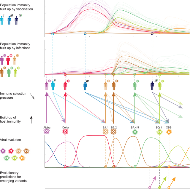
A cross-scale analysis of acquired population immunity maps evolutionary forces of SARS-CoV-2 and predicts near-future changes of viral variants, based on molecular data and time-resolved surveillance.
Graphical Abstract
Introduction
Two classes of molecular adaptation have been observed in the evolution of SARS-CoV-2 to date. Multiple mutations carry intrinsic changes of viral functions, such as increasing the binding affinity to human receptors1, the efficiency of cell entry2,3, or the stability of viral proteins4,5. Other mutations, referred to as antigenic changes, decrease the neutralizing activity of human antibodies6–10, thereby reducing the immune protection against secondary infections11,12. The strains descending from a given mutant strain define a clade of the evolving viral population. Several of these molecular changes had drastic evolutionary and epidemiological impact, inducing global turnover of viral clades and concurrent waves of the pandemic. Since the start of the pandemic, 7 major evolved variants successively gained global predominance: Alpha and Delta in 2021, the Omicron variants BA.1, BA.2, BA.4/5, BQ.1, and XBB since 2022. These were named Variants of Concern (VOCs) by the World Health Organization13; other VOCs gained temporary regional majority. Several studies reported fitness advantages of VOCs inferred from epidemiological trajectories and comparative functional studies3,14–17. Importantly, however, the evolutionary impact of antigenic changes is time-dependent, because it depends on previously acquired population immunity: a larger amount of previous infections or vaccinations increases the global fitness advantage of an antigenic escape mutation. Specifically, multi-strain epidemiological models and simulations suggest that vaccinations can favour the emergence of escape variants18–21 and influence the turnover of circulating clades22,23; effects of this kind have been reported for some clades of human influenza24. In the case of SARS-CoV-2, pandemic infection and massive vaccination programs, with a global count of >10 billion vaccinations and >700 million confirmed cases up to 01-03-202325, have built up partial population immunity, but its feedback on viral evolution has not been quantified. This leads to the central questions of this paper: what is the feedback of vaccination and infection on the subsequent turnover of SARS-CoV-2 clades, and how can this information be harvested for evolutionary predictions? To address these questions, we infer a data-driven fitness model for SARS-CoV-2 variants with distinct components of intrinsic fitness and antigenic fitness induced by vaccination and infection.
Results
Evolutionary, epidemiological and immune tracking of SARS-CoV-2.
As a basis for our fitness model, we track time-resolved data of SARS-CoV-2 in a set of 13 regions (countries or US states) that satisfy uniform criteria of data availability for the period of main interest for this study (spring 2021 to present; these criteria are detailed in Methods). First, we obtain the cumulative population fractions of reported infections and of primary, booster and bivalent-booster vaccinations25,26. These data show that population immunity rose sharply during the SARS-CoV-2 pandemic, first primarily by vaccination, later also by more frequent infections (Figure 1A).
Figure 1. Evolutionary, epidemiological, and immune tracking of SARS-CoV-2.

(A) Cumulative population fractions of infections and of primary, booster, and bivalent booster vaccinations; data from all longitudinally tracked regions of this study (thin lines) and region-averaged trajectories (thick lines). A list of regions and selection criteria are given in Methods.
(B) Frequency trajectories for the ancestral clade (1), 7 major variant clades (Alpha, Delta, BA.1, BA.2, BA.4/5, BQ.1, XBB), and 5 global minor variant clades (BA.4.6, BA.7, BM.1.1, BN.1, CH.1); regional data (thin lines) and region-averaged trajectories (thick lines). Color bars mark the succession of major variants.
(C) Timed, global strain tree of SARS-CoV-2 with strains colored by variant. Variants are annotated at the inferred time of their emergence.
(D) Neutralisation titers, , for test strains of different variants () assayed in different immune classes of infection () and vaccination (). Numerical values are given in Table S1; the inference procedure is described in Methods.
Second, we track the evolution of SARS-CoV-2 from a set of >8M quality-controlled SARSCoV-2 sequences obtained from the GISAID database27. Sequences are assigned to genetic clades using a standard set of amino acid changes28; time-dependent clade frequencies, , are inferred from strain counts smoothened over a period of 30 days in each region (Figure 1B). Here, 1 denotes the set of clades circulating prior to Alpha, including the wild type (wt) and the early 614G mutation in the spike protein. A sequencebased, timed tree shows the genealogical relationships between these clades (Figure 1C; see Methods for details of tree reconstruction). The evolutionary tracking of SARS-CoV-2 displays the well-known clade shifts to successive major variants, 1–Alpha, Alpha–Delta, Delta–BA.1, BA.1–BA.2, BA.2–BA.4/5, BA.4/5–BQ.1, and BQ.1–XBB. The variants BA.4 and BA.5 are treated as a single clade, because they have identical spike proteins. Starting in 2022, we note an increased diversity, with multiple sub-clades of BA.2 and BA.4/5 circulating simultaneously at significant frequency.
Third, we record the antigenic evolution of SARS-CoV-2 from molecular cross-immunity data between variants. Cross-immunity induced by a primary infection against subsequent infections by related pathogens is routinely tested by neutralisation assays, which measure the minimum antiserum concentration required to neutralise the second antigen. Relative, inverse concentrations are reported as serum dilution titers; here we use logarithmic titer values, (with base 2). For SARS-CoV-2, recent work7–9,29–32 has established a matrix of titers, , measuring neutralisation of variant in immunisation class (Table S1). These immunisation classes distinguish infections by different variants (), as well as primary, booster, and bivalent booster vaccinations (). Together, these data provide a coarse-grained cross-immunity landscape of SARS-CoV-2 (Figure 1D). Infection-induced cross-immunity titers are maximal when primary infection and secondary challenge are by the same variant; antigenic evolution generates a gradual decline in subsequent variants. Cross-immunity induced by wt-based vaccines declines in a similar way, for primary vaccination mostly in the clade shifts from Alpha to BA.1, for wt boosters in the shifts from BA.1 to XBB. For bivalent boosters, significant titer drops are first observed in the currently most advanced variants XBB and CH.1.
Population immunity trajectories.
Recent work for SARS-CoV-2 has shown that neutralisation titers predict the cross-immunity , defined as the relative drop of secondary infections in human cohorts. This dependence is approximately given by a Hill function11,12, , for secondary infections shortly after the primary immunisation. This form is consistent with the underlying biophysics of antibody-antigen binding and with results for other viral pathogens33–36. The intra-host concentration of neutralising antibodies decays exponentially with time after immunisation37,38. This translates into a linear titer reduction, such that the cross-immunity at later times is given as . Together, cross-immunity depends in a predictable, nonlinear way on neutralisation titer and on time since primary immunisation.
To track population immunity over time, we combine the cross-immunity factors with the population rates of new infections and vaccinations, , in different immunisaton classes . Here, clade-specific infection data are obtained by multiplying the total rate of new infections reported in each region, (i.e., the time derivative of the cumulative population fraction shown in Figure 1A) with the simultaneous viral clade frequencies, (Figure 1B). Together, we infer the population cross-immunity against clade by immunisation in class ,
| (1) |
Figure 2 shows the resulting regional and region-averaged population immunity trajectories for multiple immune classes and viral variants. These trajectories integrate three factors of change: increase by recent infections or vaccinations, and decrease by intra-host antibody decay and viral escape evolution.
Figure 2. Population immunity trajectories.

The time-dependent population immunity, , is shown for the major variants, (coloured lines), and the immune classes, (indicated by pictograms), relevant for this study. Trajectories for each immune class start at the dashed line (top: vaccination-derived immune classes, ; bottom: infection-derived immune classes, ). Thin lines show region-specific, thick lines region-averaged trajectories.
Fitness model.
To quantify the feedback of cross-immunity on viral evolution, we use a minimal, computable fitness model,
| (2) |
where is the absolute fitness, or epidemic growth rate, of a viral variant. We compute fitness at the level of variants, neglecting fitness differences between strains within a clade. Absolute fitness depends on the effective reproductive number (the average number of new infections generated by an infected individual) and on the distribution of generational intervals (the time between infection and transmission)39,40 (Methods). Here, we write fitness as the sum of a time-independent intrinsic component, , and of time-dependent antigenic components, (Methods). Each component is proportional to the corresponding cross-immunity factor with a weight factor for each immune class . Hence, antigenic selection is generated by cross-immunity differences between competing strains. The relative fitness, or growth rate difference to the mean population, of a given variant governs its adaptive frequency change as predicted by the fitness model,
| (3) |
where . This type of fitness model has been established for evolutionary predictions of human influenza22,41,42 and is grounded in multi-strain epidemiological models43–45. Here we develop model-based predictions based on human cross-immunity data, systematically including vaccination effects. In this model, equations (1), (2), and (3) describe the co-evolution of the viral population and human population immunity. The minimal fitness model does not account for differences in cross-immunity between human hosts in the same immune class (for example, through differences in immunodominance46) and for correlations between multiple prior infections (antigenic sin47).
Model training and validation.
To calibrate the fitness model, we use empirical fitness values inferred from observed frequency trajectories. Assuming that large-scale frequency shifts of viral clades are adaptive processes, we apply the reverse of equation (3), , to the tracked frequency data (Figure 1B). Empirical frequency and fitness trajectories are distinguished by a hat from their model-based counterparts. We infer the maximum-likelihood (ML) fitness model by comparing these empirical fitness trajectories with their model-based counterparts, , computed from equations (1) and (2). The model-based fitness values are derived from regional population immunity trajectories for all regions included in the analysis. We use a minimal antigenic model with just two dynamical parameters (Methods): a uniform for vaccination and boosting (downweighted in the shifts Delta-BA.1 and later, to account for double infections48) and a uniform for all infection classes (upweighted by a factor b to correct for relative underreporting; this factor is updated from past infection data).
A region- and time-resolved analysis is essential for the accurate inference of selection, because it allows to delineate spatial and temporal variation of selection. Growth differences between regions reflect inhomogeneous conditions of contact limitations, surveillance, geography, and population structure that are not included in the minimal model. In a given region, however, variants compete under more homogeneous conditions and growth rate differences, , reflect selection. Our model calibration procedure focuses on the frequency trajectories of major variants, which allow a reliable evaluation of empirical selection coefficients in all regions of this study (Data S1). Because the temporal variation of model selection coefficients in a given region depends only on antigenic selection, we can separately infer antigenic and intrinsic selection components. Details of the inference procedure are given in Methods; ML model parameters and selection coefficients for all clade shifts are reported in Table S2 and S3.
In Figure 3A, we plot the resulting ML fitness trajectories, , against the corresponding empirical trajectories (dots) for the sequence of major variants 1,Alpha,..., BQ.1. These trajectories are averaged over all 13 regions; region-specific results are given in Figure S1. We obtain a remarkable data compression: the antigenic fitness computed from equation (2) reproduces the empirical fitness changes in multiple regions and clade shifts.
Figure 3. Fitness trajectories and selection breakdown for major clade shifts.

(A) Relative fitness of successive major variants in 7 completed clade shifts (1–Alpha, ... BA.4/5–BQ.1). Model-based trajectories for each variant, (lines) are shown in the time interval between origination and loss; empirical fitness values, (dots) are inferred from the frequency trajectories of Figure 1B. All trajectories are averaged over 13 regions; see Figure S1 for regional trajectories. Color bars mark the succession of major variants.
(B) Breakdown of selection for each clade shift. Intrinsic selection coefficients, (black), and antigenic selection coefficients in marked immune classs, (coloured), as inferred from the ML fitness model (bars: region- and time-averaged value for each crossover; arrows: region-averaged rms temporal change, , with marked direction; confidence intervals are given in Table S3).
The antigenic fitness seascape.
Our fitness model posits that time-dependent selection is predominantly antigenic, i.e., caused by differences in population immunity against competing variants. Antigenic selection generates two opposing effects. A high rate of recent infections or vaccinations induces increasing positive selection for an antigenic escape variant by strengthening population immunity against previous variants. Conversely, waning of population immunity against ancestral variants, as well as immunity generated by the invading variant against itself, can decrease antigenic selection over time. Here, we trace both of these effects in the dynamics of clade shifts. From the fitness model, we compute the time-dependent selection coefficient between ancestral and invading variant, , and its decomposition into intrinsic and antigenic selection, with (arrows in Figure 3B); this computation uses past epidemic data (Figure 1, 2). For the Alpha–Delta shift, we find net increase of selection, caused predominantly by the concurrent buildup of vaccination-induced immunity against Alpha. For the subsequent shifts Delta–BA.1, BA.2–BA.4/5, and BA.4/5– BQ.1, immune waning and self-immunity generate a net decrease of selection. For the early shift 1–Alpha, selection is only weakly time-dependent because ancestral and invading variant are antigenically similar population immunity is still small; for BA.1–BA.2, selection components of opposite time dependence generate similarly small net effect. This pattern is confirmed by the empirical selection pattern inferred from regional clade frequency data (Figure S2). During the Alpha–Delta shift, selection increases with time in 16/16 regional trajectories; during the Delta–BA.1, BA.2–BA.4/5, and BA.4/5–BQ.1 shifts, selection decreases in 35/37 trajectories. Hence, compared to a reference of time-independent selection, the Alpha–Delta shift runs at an accelerating speed, the three subsequent shifts at a decelerating speed. In all 4 cases, the temporal variation of selection is statistically significant ( for each shift; two-sided Wald test) and substantial (a linear regression gives ). In the remaining shifts, the time dependence of selection is insignificant or weak ( for 1–Alpha, for BA.1–BA.2).
To test our fitness model and selection inference, we examine whether intrinsic selection can produce a comparable signal of time-dependence. Sources of intrinsic selection include changes in transmissibility, intra-host replication rate, and pathogenicity, which affect the basic reproductive number and the distribution of generation intervals. Such changes have been reported for some of the early major variants1,3,49,50. In Methods, we show that the resulting intrinsic selection is coupled to absolute growth in some cases (Figure S3). Because absolute growth depends on time through multiple factors including temperature, population density, and non-pharmaceutical containment measures, this coupling could induce time-dependent intrinsic selection, at variance with our fitness model40. To assess this possibility, we evaluate the empirical variation of absolute growth along regional trajectories. We find only a small co-variation with selection and, hence, no evidence for time-dependent intrinsic selection (Methods, Figure S3). We conclude that antigenic changes are the dominant source of time-dependent selection, corroborating our minimal fitness model and the resulting decomposition of selection (Figure 3B). Similarly, our inference of selection is robust under time-dependent non-pharmaceutical interventions (Methods, Figure S3).
Intrinsic, infection-induced, and vaccination-induced selection.
The ML fitness model provides a breakdown of the selection forces driving the observed sequence of major clade shifts (Figure 3B). Intrinsic selection is strong and positive in the pre-BA.2 shifts, with average selection coefficients between invading and ancestral variant, consistent with strong functional differences observed between early variants3,51 (Table S3, all selection coefficients are given in units d−1). In the post-BA.2 shifts, intrinsic selection is inferred to be small (a recent exception, XBB.1.5, will be noted below). Antigenic selection follows an opposite trend: the average selection coefficients between invading and ancestral variants are initially small but reach values in all post-Alpha shifts, except BA.1–BA.2. The recent decline, from for Delta–BA.1 and BA.2–BA.4/5 to for BA.4/5–BQ.1, reflects decreasing infection and vaccination rates towards the end of the pandemic, as well as waning protection from earlier immunisations. Consistently, the empirical total selection declines from its peak value for Delta–BA.1 to for BA.4/5–BQ.1. That is, evolution decelerates in the transition to an endemic state.
Of particular interest is the pattern of vaccination-induced antigenic selection, which maps the feedback of vaccination on the subsequent evolutionary trajectory of the virus (Figure 3B). Primary vaccination contributes substantial positive selection, , in the shifts Alpha–Delta and Delta–BA.1, which are the main steps of antigenic escape from the wt-based vaccine (Figure 1B). Booster vaccinations have increased breadth compared to primary vaccinations8,9,52,53 (Table S1, Figure 1D); that is, they induce higher cross-immunity and initially weaker selection for antigenic escape. In the Delta–BA.1 shift, boosters even generate a negative selection coefficient , because they remove cross-immunity differences and antigenic selection generated by the preceding primary vaccination. Positive selection is inferred for the post-BA.2 shifts, when the virus partially escapes from booster-induced immunity (Figure 1D). Similarly, positive selection induced by bivalent boosters is first seen in the new variants XBB and CH.1 and is expected to be peaked in the post-BQ.1 shifts (see Figure 5 below).
Figure 5. Antigenic selection profiles constrain emerging variants.

(A–E) Antigenic landscapes. Each family of landscapes shows neutralisation titers and cross-immunity factors, (dots), for a given majority variant as antigenic background and competing minority variants, in all immune classes relevant for the next clade shift. Yellow circles mark a “standard” mutant, as described in the text; data of the background variant and the standard mutant are joined by lines.
(F) Antigenic selection profiles. Predicted antigenic selection trajectories of the standard variant against the background majority variant and their breakdown into immune classes, (stacked areas), are shown for successive background variants (horizontal color bars). Posterior selection profiles of observed variants are shown at their time of emergence (stacked bars). The last panel shows the predicted profile for the future clade shift away from XBB.
Vaccination- and infection-induced selection are statistically significant parts of the calibrated fitness model for SARS-CoV-2 (Figure 3B); partial models with only one component have a strongly reduced posterior likelihood (differences in model complexity are accounted for by a Bayesian information criterion; see Methods and Table S2). These results show that vaccination and previous infections induced sizeable antigenic selection on circulating SARS-CoV-2 variants and modulated the speed of successive clade shifts. However, the fitness model and our data analysis do not predict any simple relation between vaccination coverage and the speed of evolution. This is because cross-immunity classes are correlated: fewer vaccinations lead to more infections, generating a buildup of cross-immunity in other classes and complex long-term effects.
Predicting short-term evolution.
The post-BA.2 evolution of SARS-CoV-2 is characterised by the prevalence of antigenic selection (Figure 3B) and by the emergence of multiple, competing antigenic variants. Besides the major variants BA.4/5, BQ.1, and XBB, these include the clades BA.4.6, BF.7, BN.1, and CH.1, all of which show initial growth and antigenic differences from their parent clade (Figure 1CD). Can the fitness model predict the short-term evolution of such complex viral populations? To address this question, we first plot the timed tree of all strains descending from BA.2, colouring each isolate by the relative fitness computed from the antigenic fitness components at the time of sampling, (Figure 4A). The fitness model is seen to predict subsequent frequency shifts of clades: high fitness signals frequency increase, low fitness frequency decline.
Figure 4. Predicting short-term evolution.

(A) Strain tree of BA.2 and descendent variants; strains are colored by model-based, clade- and time-dependent relative fitness, .
(B) Short-term frequency change. We compare predicted changes, , with posterior empirical changes, , over periods in all longitudinally tracked regions for 8 variants with initial frequencies (ascending segments), (descending segments).
(C) Predominance shifts. We compare predicted and posterior trajectories of reduced fitness, (dashed) and (solid), over periods , starting from the emergence of new variants (marked above each panel); see text. Bold lines highlight variants predicted to outcompete all other variants co-existing at their time of emergence (i.e., to reach reduced frequencies ).
To assess the predictive power more quantitatively, we compare predicted frequency changes, , with their observed counterparts, , for a prediction period and for post-BA.2 variants (Figure 4B). To compute the frequencies , we evaluate the fitness model at time , using tracking data and parameter inference only up to that time (Methods). We evaluate regional frequency trajectories of each clade at multiple time points, including periods of observed increase and of decrease . Predicted and observed frequency changes are seen to be strongly correlated (coefficient of determination ); frequency increase is correctly predicted in 142/182 cases, decline in 144/149 cases.
Next, we test whether the fitness model can flag new variants of concern at an early point of their frequency trajectory. Whenever a new variant emerges at global frequency , we predict its subsequent evolution in a window of 200d, together with all variants present at the start of prediction with frequency > 0.005 (Methods). Figure 4C shows reduced frequency trajectories, , which are defined in these sets of competing variants. We compute predicted trajectories (dashed lines) from the antigenic fitness model at the start of each window, using tracking data and parameter inference only up to that time, and compare them to empirical trajectories tracked from posterior data (solid lines). Of 7 variants with available antigenic data, BF.7, BQ.1, and XBB are correctly predicted to outcompete all variants present at the time of their emergence, i.e., to reach reduced frequencies > 0.5, within 200d. The other 4 variants are correctly predicted to remain below majority within that time interval. We note that XBB shows a pronounced fitness increase two months after emergence. This can be traced to the subclade XBB.1.5 with the additional intrinsic change S:S486P, which increases ACE2 binding54.
Selection windows and antigenic profiles of new variants.
The preceding analysis predicts predominance changes in a set of variants coexisting at the start of prediction, but it remains agnostic about variants that emerge later. The genetic identity of new variants is highly stochastic and unlikely to be predictable55. However, the antigenic characteristics of successful variants are constrained by the history of previous infections and vaccinations. According to our fitness model, temporally localised windows of strong antigenic selection are generated when high population immunity coincides with high expected loss of cross-immunity on the steep flank of a Hill landscape in one or more immune classes.
To exploit this constraint for predictions, we first display the antigenic evolution on cross-immunity landscapes (Figure 5A–E). For each of the major variants Delta, BA.1/2, BA.4/5, BQ.1, and XBB as antigenic background, a family of landscapes maps the titer and the cross-immunity factor for the background major variant and the competing minor variants (colored dots) in all immune classes relevant for the next evolutionary step. Here we treat the antigenically similar variants BA.1 and BA.2 as a single antigenic background (Table S1). From these landscapes, we can read off the class-specific antigenic advance or titer drop, , and the resulting incremental escape from cross-immunity, , of each competing variant compared to the background variant. A hypothetical “standard” mutant with a uniform against the background variant is marked by yellow circles; this antigenic advance is close to the average of observed mutants. In the post-BA.2 period (cf. Figure 4), we compute the resulting antigenic selection profile, i.e., the time-dependent selection coefficient and its breakdown into immune classes, for the standard mutant against the successive major variants (Figure 5F, shaded areas). This reveals a strongly time-dependent pattern: selection in a given immune class builds up by recent infections or vaccinations; it gets depleted by immune waning and, even more rapidly, by the shift to a new major variant that has largely completed the immune escape in that class.
The antigenic selection profiles of Figure 5B predict antigenic characteristics of new, yet unseen variants that can successfully escape population immunity. The predicted profile is conditional on the new variant’s emergence at time t; the computation uses tracking and antigenic data up to that time. Remarkably, the observed profiles of new high-fitness variants at their actual time of emergence are in broad agreement with the predicted pattern (Figure 5F, stacked bars). That is, the overall amplitude and the directions of antigenic escape evolution are constrained by selection computable from prior data. Three immune classes, booster vaccinations and infections by BA.1 and BA.2, drive the antigenic shift BA.2–BA.4/5. Primary vaccinations are no longer relevant for this shift, because BA.1 and BA.2 have already largely completed the immune escape in this class (Figure 5A). The variant BA.4/5 escapes only partially in the classes BA.1/2 and bst. Hence, these classes remain relevant for the variants emerging on the antigenic background of BA.4/5, including BA.4.6, BF.7, and BQ.1, while selection induced by BA.4/5 infections is building up. This class, together with BQ.1 infections and bivalent booster vaccinations, governs the following variants XBB and CH.1, which emerge on the antigenic background of BQ.1.
All of these post-BA.4/5 variants show pronounced convergent evolution in few epitope sites; this canalisation of genome evolution has been linked to immune imprinting from previous infections or vaccinations10. Escape effects of such mutations, as measured by deep mutational scanning (DMS), can serve as input to our antigenic selection profiles and growth predictions (Methods). Specifically, the post-BA.4/5 variants differ from their recent ancestor BA.4/5 in up to 6 point mutations in the receptor binding domain, some of which show large escape effects from BA.4/5 breakthrough infections10. These effects explain the large antigenic advance of BQ.1 in immune class (Figure 5C) and the resulting fitness advantage against the competing strains BA.4.6 and BF.7 (Figure 4C). However, the initial antigenic advance and the resulting fitness gain of the recombinant variant XBB against BQ.1 (Figures 5D, 4C) is larger than expected from the sum of DMS escape effects of its point mutations (Methods).
The next shift, which will take place from an XBB background, is predicted to be driven by bivalent booster vaccinations, BQ.1 infections, and a smaller component of XBB infections reflecting reduced case numbers (Figure 5E). We note that the predicted profiles list the spectrum of immune classes inducing selection for new variants. Given the increasing differentiation of population immunity, we also expect variants that carry antigenic change in some but not all of these classes.
Discussion
Here we have established a data-driven, multi-component fitness model for the evolution of SARS-CoV-2. The model establishes a computable, cross-scale analysis of how immunity shapes evolution: molecular interactions between protective antibodies and the viral proteins, measured by neutralization assays, govern the immune protection of individuals11,12; cross-immunity data, together with epidemiological and sequence data, can be scaled up to population immunity; trajectories of population immunity shape fitness seascapes, on which viral variants compete for evolutionary success. By applying this model to tracked evolutionary trajectories in multiple regions, we have quantified intrinsic and antigenic selection driving the genetic and functional evolution of SARS-CoV-2. In particular, primary vaccination impacted on the speed of global clade shifts in 2021; booster vaccination provided higher cross-protection in the same period, but generated significant selection for antigenic escape only several months later (Figure 3). These results underscore that vaccine breadth is important for constraining antigenic escape evolution. More broadly, they highlight the need to integrate evolutionary feedback into vaccine design.
Three global trends in the recent evolution of SARS-CoV-2 are revealed by our analysis. First, antigenic selection has increased in relative strength and has broadened its target. That is, primary infection by distinct viral variants has generated an increasing number of immune classes and antigenic selection components; in parallel, multiple competing antigenic variants have appeared in recent shifts (Figure 3, Figure 5). Second, intrinsic selection has broadly decreased in strength, and some compensatory intrinsic changes have been reported56. Third, the overall speed of clade shifts has decreased substantially since the peak of the pandemic. These trends mark the transition from initial, post-zoonotic adaptation of the virus to evolution in a well-adapted endemic state. A plausible end point of this transition becomes clear by comparison with influenza, a long-term endemic virus in humans. The evolution of influenza is a continuous adaptive process driven by antigenic selection, where multiple variants with different antigenic profiles compete for predominance57. In contrast, non-antigenic mutations in influenza proteins are under broad negative selection; observed changes often compensate the deleterious collateral effects of antigenic evolution on conserved molecular traits, including protein stability and receptor binding55,57,58.
Looking forward, our analysis establishes methods to predict the short-term evolution of SARS-CoV-2. The antigenic fitness model predicts how likely emerging variants will rise to predominance in the population of circulating strains, provided cross-immunity data for these variants are available at the time of prediction (Figure 4). Antigenic selection profiles for new variants, which build up and can be computed even prior to their emergence, constrain the directions of likely antigenic evolution (Figure 5). Such profiles can serve to identify informative immune cohorts for antigenic surveillance by neutralisation tests. Deep mutational scanning10,59 and high-throughput in-vitro evolution56,60 have recently been established to map the genetic profile of SARS-CoV-2 evolution, including the genomic distribution of likely escape mutations, as well as their antigenic and receptor binding effects. These approaches may eventually provide genotype-phenotype maps for antigenic evolution61. Combined with our population-level antigenic selection profiles, such data can further constrain the likely paths of escape from human immunity.
In a broader context, our results show how the coupled dynamics of human population immunity and viral evolution can be digested into predictions for global pathogens. The approach addresses a notorious problem: sequence-based data of the evolving pathogen alone, including the genetic changes and the initial growth rates of emerging mutants, provide only limited information on their eventual fixation and evolutionary impact57,62. This is because antigenic escape evolution is complex: a given escape mutation has a spectrum of effects in multiple classes of population immunity (Figure 5). Within each class, selection is epistatic and timedependent: pressure for escape is peaked on the steep flanks of cross-immunity Hill functions, and its strength is modulated by new infections or vaccinations and by immune waning. We have shown that immune selection is computable despite this complexity, given integrated molecular and epidemiological data. Thus, our analysis calls for continued, comprehensive surveillance of SARS-CoV-2, combining tracking of genome sequences and incidence data with timely cross-immunity analysis. This input will be critical for our ability to predict antigenic escape evolution and to harvest such predictions for pre-emptive vaccine design.
Limitations of the study.
Our analysis uses population immunity trajectories inferred by combined tracking of epidemiological, sequence, and cross-immunity data. Undersampling or biases in any of these source data limit the accuracy of the inference. Sequencing biases between clades also affect the inference of empirical fitness. To mitigate these effects, the longitudinal analysis is carried out in a set of 13 regions with comparable data quality (selection criteria are detailed in Methods). Hence, the breakdown of selection components applies to the set of regions accessible to our analysis; the availability of comparable data precludes a fully global model-based inference of selection. Data on cross-immunity between viral variants is aggregated from multiple studies (Methods, Table S4). Biases and sensitivity differences between datasets propagate into the model-based fitness differences between viral variants.
The minimal fitness model uses a simplified representation of immune classes, enabling the use of available neutralisation data for cross-scale analysis of population immunity. The model effectively averages over the variation of cross-immunity between human hosts within the same immune class and neglects correlations between multiple infections. In particular, as noted above, this treatment assumes that host-to-host differences in immunodominance, antigenic sin, or immune waning have only limited impact on global antigenic selection and the resulting evolutionary dynamics. Furthermore, our fitness model is derived from an underlying multi-strain epidemiological model under specific assumptions, which decouple relative fitness from absolute growth and imply additivity of antigenic and intrinsic fitness components. These assumptions are detailed in Methods; see also Figure S3 for validity checks and error margins of the selection-growth decoupling.
Our predictive analysis leverages population immunity derived from past data to signal near-future prevalence shifts between variants and to constrain antigenic profiles of emerging variants. Antigenic surveillance is the main limiting factor of these and future evolutionary predictions. More dense and timely antigenic data are required to fully assess and harvest the predictive power of the fitness model. Furthermore, a comprehensive statistical validation will require longer time series of tracked evolutionary data.
Star Methods
Resource availability
Lead Contact
Further information and requests for data should be directed to and will be fulfilled by the lead contact, Michael Lässig (mlaessig@uni-koeln.de).
Materials availability
This study did not generate new unique reagents, but raw data and code generated as part of this research can be found on public resources as specified in the Data and Code Availability section below.
Data and code availability
This paper analyzes existing, publicly available data. These accession numbers for the datasets are listed in the key resources table.
Results, and analyses can be found at https://github.com/m-meijers/Population_Immunity_SARSCOV2 and is publicly available as of the date of publication. DOIs are listed in the key resources table.
Any additional information required to reanalyze the data reported in this paper is available from the lead contact upon request.
KEY RESOURCES TABLE
| REAGENT or RESOURCE | SOURCE | IDENTIFIER |
|---|---|---|
| Deposited Data | ||
| SARS-CoV-2 sequence data | GISAID EpiCov Database | http://www.gisaid.org |
| Infection and vaccination rates | Ourworldindata | https://www.ourworldindata.org |
| Infection and vaccination rates | CDC COVID Data Tracker | https://www.covid.cdc.gov/covid-datatracker |
| Antigenic Data | References [3,7,8,10,29-32,52,53,71-91] | Supplementary Materials 1 |
| Software and Algorithms | ||
| MAFFT v7.490 | Katoh and Standley [64] | https://mafft.cbrc.jp |
| IQTree | Minh et al. [65] | http://www.iqtree.org/ |
| TreeTime | Sagulenko et al. [67] | https://github.com/neherlab/treetime |
Method Details
Antigenic data
Neutralisation assays for SARS-CoV-2 test the potency of antisera induced by a given primary immunisation to neutralise viruses of different variants. Log dilution titers measure the minimum antiserum concentration required for neutralisation,
| (S4) |
relative to a reference concentration . Hence, titer differences, or neutralisation fold changes, , measure differences in antigenicity between variants, . We note that these differences are specific to a given primary infection or vaccination (immune class) . For example, the inequality reflects the increased breadth of booster vaccinations compared to primary vaccinations. In contrast, uni-valued antigenic distances between variants, , can be computed from the titer matrix by multi-dimensional scaling methods63,64. Such distance measures average over inhomogeneities between immune classes. Here we define a matrix of titer drops ,
| (S5) |
with respect to a reference titer for each immune class, and . This procedure eliminates technical differences between assays in absolute antibody concentration. We assemble this matrix in Table S1, using primary data from different sources3,7,8,10,29–32,52,53,65–85 (see also Table S4.). We proceed as follows: (i) For matrix elements with available data, is the average of the corresponding primary measurements. (ii) If no data are available for but the conjugate titer has been measured, we use the approximate substitution , as discussed in ref. 86. (iii) If no data are available for but the titer of a closely related clade has been measured, we use the approximate substitution , which should be understood as a lower bound. Approximate substitutions are indicated by italics in Table S1.
The matrix of absolute neutralisation titers, , is then computed by equation (S5), combining the titer drops of Table S1 and the reference titers , , reported in ref. [87]. A titer difference between vaccination and booster, , has been observed in several studies8,9,52. The resulting titers are shown in Table S1; they enter the cross-immunity functions and defined below.
The decay of antibody concentration after primary immunisation has been characterised in recent work37,38. Here we describe this effect by a linear titer reduction with time after primary challenge,
| (S6) |
corresponding to an exponential decay of antibody concentration, with a uniform decay time 90d (i.e., half life ). This is broadly consistent with experimental data; we infer decay times in the range [60,170]d from several studies7,8,37,38,52. In addition, we check that varying in this range does not affect our results (in particular, the rank order of variants with respect to antigenic fitness remains unchanged).
Sequence data and primary sequence analysis
The study is based on sequence data from the GISAID EpiCov database27 available until 2023–04-01. For quality control, we truncate the 3’ and 5’ regions of sequences and remove sequences that contain more than 5% ambigous sites or have an incomplete collection date. We align all sequences against a reference isolate from GenBank88 (MN908947), using MAFFT v7.49089. Then we map sequences to Variants of Concern/Interest (VOCs/VOIs), using the set of identifier amino acid changes given in Outbreak.info28. As a cross-check, we independently infer a maximum-likelihood (ML) strain tree from quality-controlled sequences under the nucleotide substitution model GTR+G of IQTree90, using the reference isolate hCoV-19/Wuhan/Hu-1/2019 (GISAID-Accession: EPI ISL 402125) as root. For assessment of the tree topology, we use the ultrafast bootstrap function91 with 1000 replicates. Internal nodes are timed by TreeTime92 with a fixed clock rate of 8 × 10⁻⁴ under a skyline coalescent tree prior93. Consistently, variants are mapped to unique genetic clades (subtrees) of the ML tree (Figure 1C, 4A).
Frequency trajectories of variants
For a given variant , we define the smoothened count , where the sum runs over all sequences mapped to variant and is the collection date of sequence . We use a smoothening period , which gives significant weight to sequences collected at times . The empirical variant frequency is then defined by normalisation over all co-existing variants, . Frequencies are computed until the cutoff 2023–03-01, one month before data download. These frequency trajectories, evaluated separately for each region of this study, as well as averaged over regions, are shown in Figure 1B.
Infection and vaccination trajectories
Daily infection and vaccination rates for individual regions have been obtained from Ourworldindata.org25 and from CDC COVID Data Tracker26 for US states (download date: 2023–04-01). The resulting cumulative population fractions of infected individuals, together with cumulative population fractions of primary, booster, and bivalent booster vaccinations are reported in Figure 1A. Clade-specific infection rates are computed by multiplying the total daily infection rates reported in each region with the simultaneous viral clade frequencies .
Data integration for regional analysis
This study uses sequence data and epidemiological data from multiple regions for parallel analysis. Sequence data serves to infer empirical fitness trajectories for individual clades from their frequency trajectories. Epidemiological records provide input to the antigenic fitness model, equations (1) and (2). The evaluation of the fitness model, which is detailed below, integrates data of both categories and requires stringent criteria of data availability and comparability between regions.
In each region, we require the following criteria for a given clade shift: (i) The smoothened sequence count exceeds 500 sequences per day in the period from 2021–04-01 to 2022–09-01, which covers the majority clades from Alpha to BA.4/5. This criterion ensures that the empirical relative fitness, especially for minority frequencies, can be estimated with reasonable statistical errors. Most exclusions of regions based on insufficient sequence data. (ii) Both the invading and ancestral variant are majority variants in different time intervals for each of the major global clade shifts. This criterion excludes regions where other variants are predominant during the clade shifts (e.g., Brazil and South Africa had throughout the 1–Alpha shift). (iv) The empirical selection trajectory contains at least 6 measured points for the Alpha–Delta clade shift, and at least 4 measured points for later clade shifts. This criterion ensures a sufficient signal-to-noise ratio for inference of temporal variation along the trajectory. (v) The total number of reported infections exceeds 5% of the population on 2022–02-01. This criterion excludes regions with very low number of reported infections at the height of the pandemic (e.g., Japan) and ensures that cross-immunity trajectories, as given by equation (1), can be evaluated across regions with sufficient consistency. (vi) Vaccinations have been predominantly by mRNA vaccines and epidemiological records in the database are complete. This criterion ensures population immunity computed in the vaccination immune classes are comparable between regions. It excludes regions with substantial use of viral vector vaccines (e.g., the UK).
We identify a set of 13 regions that satisfy the above criteria in all clade shifts up to BA.4/5: Belgium, California (representative of US West Coast), Canada, Finland, France, Germany, Italy, Netherlands, Norway, New York (representative of US East Coast), Spain, Switzerland, US (remainder). This set is used for the longitudinal-tracking analysis of the main text (including Figures 1–5, S1). The inference of model parameters and shift-specific regional analysis (Figures S2, S3, Data S1) is performed in all regions that fulfil these criteria for a given clade shift.
Inference of empirical fitness
Using the reverse of equation (3), we infer relative fitness trajectories from regional frequency trajectories,
| (S7) |
with a time step days for evaluation of the derivative. A hat distinguishes empirical relative fitness and frequency trajectories from their model-based counterparts introduced below. For a given variant, we compute empirical fitness trajectories, , for the maximal time interval such that along the entire trajectory. The start point is the first day when . From this point, the relative fitness is recorded weekly. Single measurements are excluded when the sequence counts is . Statistical errors for relative fitness trajectories are evaluated by binomial sampling of counts with pseudocounts of 1. In Figure 3, we show trajectories of averaged over all longitudinally tracked regions; the corresponding regional trajectories are reported in Figure S1.
The selection coefficient between the invading and ancestral variant in a clade shift equals their difference in their relative fitness, . From equation (S7), the empirical selection coefficient between these variants takes the form
| (S8) |
Empirical selection trajectories for clade shifts between majority clades, , starting at a time when and running until a time when , are reported in Data S1 and Figure S2; these trajectories also serve the inference of antigenic model parameters detailed below.
The time dependence of empirical selection trajectories in the completed clade shifts from 1 to BQ.1 is analyzed in Figure S2. We evaluate two summary statistics: (i) the amount of systematic time-dependent variation of selection, defined as , averaged over regions, where is a linear regression to the ensemble of trajectories; (ii) the statistical significance of the linear regression, (two-sided Wald test). These tests show strong and significant temporal variation the 4 clade shifts Delta–BA.1, BA.2–BA.4/5, BA.4/5–BQ.1 ( and ). We find no significant time dependence for the shift 1–Alpha () and weak time dependence for BA.1–BA.2.
Cross-immunity trajectories
The antigenic, epidemic and sequence data, as described above, are combined in cross-immunity trajectories that describe the total protection in a population against a given variant , as derived from an immune class . First, the cross-immunity factor is defined as the relative reduction in infections by variant induced by (recent) immunisation in class . As shown in recent work11,12, absolute titers of SARS-CoV-2 neutralisation assays can predict cross-immunity, with
| (S9) |
This relation has been established in ref. 11 with constants and . It takes the form of a thermodynamic Hill function, consistent with the fact that functional, near-equilibrium binding of antigens and antibodies is a major determinant of neutralization. The resulting cross-immunity factors include antibody decay, as given by equation (S6). Hence, they depend on the time since primary immunisation,
| (S10) |
These factors enter the population cross-immunity functions , equation (1),
| (S11) |
where are the time-dependent population rates of immunisations in a given immune class. The cross-immunity functions inferred in this study are plotted in Figure 2; they enter all evaluations of the fitness model, equation (2) (Figures 3–5, S1).
Minimal fitness model
The analysis of the main text is based on a fitness model with two main components. Intrinsic fitness depends on the the clade-specific basic reproductive number, . Antigenic fitness is mediated by population cross-immunity, which enters the epidemic dynamics through a reduction of the susceptible population and a proportional reduction of the effective reproductive number, . In a multi-strain epidemic, we describe this reduction by a multiplicative superposition of immune classes,
| (S12) |
This form accounts for the bookkeeping of multiple (breakthrough) infections in an individual’s immune history in an approximate way45 and has the correct asymptotics when becomes large. The weight factors rescale the cross-immunity functions computed from reported data to their actual fitness effect. These factors are free model parameters; their inference will be detailed below.
Linking reproductive number to epidemic growth requires a model for the distribution of time intervals between subsequent infections in a transmission chain (generation time intervals). Here we use the established form of a Gamma distribution with uniform mean and variance (i.e., with shape parameter ); deformations of this form will be discussed below. The clade-specific growth rate (absolute fitness) is then given by40,94
| (S13) |
For SARS-CoV-2, we use basic parameters and obtained from averaged literature values as reported in ref.95. In this parameter regime, the growth rate is well approximated by the form given in the main text,
| (S14) |
as shown in Figure S3A. This form becomes exact in the limit of uniform generation time intervals .
Combining equations (S12) and (S14), we obtain the fitness model of the main text,
| (S15) |
where and are the intrinsic and antigenic fitness components, respectively. Fitness differences (selection coefficients) between clades, , take the form
| (S16) |
The minimal model has three simplifying properties. (i) Intrinsic and antigenic selection enter additively; i.e., there is no epistasis between these components. (ii) Antigenic fitness is additive in the immune classes. This is consistent with the assumption that in an infection chain, a viral lineage rapidly samples hosts randomly distributed over immune classes. (iii) Selection coefficients decouple from absolute growth, i.e., are invariant under a uniform rescaling . This is important for the robustness of our inference method under non-pharmaceutical interventions, as discussed below.
Model validation
Multiple phenotypes and functions affect the viral life cycle, including the stability of viral proteins, binding to receptors of human cells, intra-cellular replication and defence against innate immunity, and transmission between hosts. All of these can be the target of intrinsic selection, by modulating the reproductive number and the distribution of generation intervals. Here we introduce three simple evolutionary deformations of the infection dynamics and analyse their consequences for the fitness model.
Changes in reproductive number. A mutation of the virus increasing its transmissibility between hostscan be assumed to increase the basic reproductive number , while keeping the generation parameters and invariant. In Figure S3A, we plot the selection coefficient of a mutant clade with increased basic reproductive number, , as a function of the antigenic selection under the minimal model, , for three values of (corresponding to three absolute rates of epidemic growth, ) with basic generation parameters and . In good approximation, selection is seen to be additive and independent of absolute growth, with , as given by the minimal model, equation (S16).
Changes in mean generation interval. A mutation increasing the rate of intra-host replication can shorten the time to the start of transmission, while keeping the infectious period unchanged. This type of change can approximately be described by a decrease of at constant and (Figure S3B). The resulting selection coefficient remains approximately additive, , but the intrinsic selection coefficient becomes dependent on absolute growth. This coupling is not described by the minimal model and, if absolute growth depends on time, introduces a time-dependence of intrinsic selection.
Correlated changes of infection parameters. Here we consider mutations that increase pathogenicity by prolonging the infectious period. This type of change can approximately be described by a correlated increase of , and , such that the time to the start of transmission remains unchanged but the end of transmission is delayed (Figure S3C). The resulting selection coefficient is additive and consistent with the minimal model, , where depends on the change in the infectious period, but is approximately independent of absolute growth.
Together, mutations between variants that affect the viral replication cycle can introduce a coupling between absolute growth and selection and, in turn, generate time-dependent intrinsic selection that confounds our inference of antigenic selection as the time-dependent component of the total selection coefficient. The magnitude of this effect depends on the detailed mechanistic effects of mutations between variants, which are in general unknown. For three major variants relevant for this study, changes in the mean generation interval have been reported, from for Alpha to for Delta49 and from for Delta to for BA.150. To estimate the growth-selection coupling directly from empirical data, we record the time-dependent total growth rate and its correlation with selection for the Alpha–Delta and the Delta–BA.1 shifts (Figure S3F, G). We infer absolute growth trajectories,
| (S17) |
where are reported incidence values and is to be interpreted as a population mean, (Figure S3F). From these trajectories, we estimate the region-averaged temporal change, , over the duration of each clade shift; we find for Alpha–Delta and for Delta–BA.1. Next, we evaluate the systematic co-variation of selection and growth by means of a linear regression, ; we find for Alpha–Delta and for Delta– BA.1 (Figure S3G). Hence, only a small part of the time-dependence of selection, of order , can be explained by the coupling to absolute growth induced by intrinsic selection. We conclude that antigenic changes are the dominant source of time-dependent selection, in accordance with the minimal selection model, equation (S15).
Non-pharmaceutical interventions
Such measures generate changes in social behaviour that affect viral transmission, modulating the reproductive number and the distribution of generation intervals uniformly for all circulating strains. Non-pharmaceutical interventions (NPI) can have two kinds of effects: (i) Reduction of reproductive numbers. Mask wearing or social distancing can reduce transmission rates and generate a uniform, time dependent modulation of reproductive numbers, , while keeping the generation parameters and invariant (Figure S3D).
(ii) Reduction of the infectious period. Surveillance and isolation measures can also reduce the effective infectious period, generating a uniform, correlated decrease of , and (Figure S3E). Effects of this kind have repeatedly been reported during the SARS-CoV-2 pandemic95,96.
For both kinds of interventions, we compute the selection coefficient of an antigenic mutant clade against the corresponding selection coefficient under the minimal model, , for two values of the NPI constraint. We find that, while NPI can strongly affect absolute growth, selection coefficients are approximately independent of the NPI constraint. Hence, our selection inference is robust under time-dependent changes of NPI measures.
Inference of fitness model parameters and selection coefficients
The free parameters measure the fitness effect of each cross-immunity component. These parameters calibrate the model to data of real populations with complex population structure, including incidence structure and variation of infection histories, as well as heterogeneity in the monitoring of infections. To avoid overfitting, we use a minimal model with just 2 global antigenic parameters: (i) A basic rate translates cross-immunity generated by vaccination into units of selection. We infer a value for the Alpha-Delta shift and a lower value for all later shifts (Table S2); this value is used for all predictions. This can be seen as a heuristic to account for the effect of double infections48, which increase cross-immunity and decrease cross-immunity differences between variants. (ii) A uniform rate for all infection classes, , includes a weight factor accounting for underreporting of infections relative to vaccinations. We infer an initial value for all shifts up to BA.2 (inferred from data up to the completion of Delta–BA.1; the shift BA1–BA.2 involves only small antigenic effects). For the post-BA/2 period, we infer a time-dependent factor from data in a sliding window . This value is used for predictions from time t into the future (Figure 4, 5). The selection breakdown for individual shifts (Figure 3, S1, Data S1, Table S3) uses posterior values inferred from data until completion of each shift: for pre-BA.2 shifts, for BA.2–BA.4/5, for BA.4/5–BQ.1 (Table S2).
The model parameters are trained on regional trajectories of selection coefficients for the majority clades. We infer the ML fitness model by aggregation of log likelihood scores evaluated for these trajectories. We use the score function
| (S18) |
for a single empirical selection trajectory and its model-based counterpart . The expected square deviation is ; the first term describes the sampling error of sequence counts, which enters frequency and empirical selection estimates, the second term summarises fluctuations unrelated to sequence counts. The total log likelihood score is the sum , which runs over all shifts in a given time interval and all included regions. We evaluate the ML score and the corresponding BIC score97 relative to a null model of time-independent selection (Table S2). The 95% confidence intervals of the inferred parameters are computed by resampling the empirical selection data with fluctuations . We infer a decrease in the ML vaccination parameter ( with ), which is consistent with the interpretation of the parameter as weighting factor accounting for double-infections. Similarly, we infer a ML infection weight parameter ; the function gradually increases in 2022, interpolating between the end-of-shift values . This pattern is consistent with accounting for underreporting (see above). The ML selection components resulting from our inference are reported in Figure 3B and Table S3.
The inference procedure works as follows: (i) For the pre-BA.2 clade shifts, which are characterised by strong data heterogeneity between regions, we decompose model-based and empirical selection trajectories into temporal mean and change, and , where brackets denote time averages over the trajectory for a given region. In a first step, we infer the ML antigenic parameters and from the within-region selection changes , using the partial score . Importantly, this inference step yields the ML antigenic model parameters and the resulting ML antigenic selection components, , independently of intrinsic selection. In a second step, we infer the intrinsic selection for each shift as the difference between empirical selection and ML antigenic selection, , where the double brackets denote averaging over time and regions. (ii) For the post-BA.2 clade shifts, where frequency tracking data are less heterogeneous between regions, we can use a singlestep inference procedure with the score function (S18). On the other hand, reported incidence numbers become highly heterogeneous in this period. Therefore, we average the population immunity functions for infection-derived immune classes over the included regions. The post-BA.2 data turn out to be well described by a ML antigenic fitness model . This is important for predictions: computing the initial fitness of an emerging variant involves tracking data only of previous variants (Figure 4B, 5F). Predictive analysis in this period uses a weight factor inferred from data in the time window with daily updates from (start of the clade shift BA.2–BA.4/5); window segments before this date are weighed in proportionally with the initial value .
Significance analysis of the fitness model
To assess the statistical significance of our inference, we compare four fitness models of the form of equation (2): the full model used in the main text (VAC+INF: antigenic selection by vaccination and infection, intrinsic selection), two partial models (VAC: antigenic selection only by vaccination, intrinsic selection; INF: antigenic selection only by infection, intrinsic selection), and a null model (0: intrinsic selection only). We infer conditional ML parameters for each model and we rank models by their ML score difference to the null model, (Table S2). An alternative ranking by BIC score97, which contains a score penalty for the number of model parameters, leads to the same result. Both scores are reported separately for the pre-BA.1 period and for the full inference period.
We obtain the following results: (i) The antigenic fitness models VAC+INF and INF have significantly higher scores than the null model, which shows that the empirical selection data are incompatible with time-independent selection. (ii) The full model has a significantly higher score than any of the other models. Hence, both vaccination and infection are significant components of antigenic selection. (iii) The partial antigenic model VAC has a higher score than INF for the pre-BA.1 shifts, but a lower score than the null model in the post-BA.2 period. Hence, vaccinations explain a substantial part of the pre-BA.1 pattern, but vaccinations alone do not capture the later data.
In summary, we infer a statistically significant fitness model with few, global parameters from sequence and epidemiological data aggregated over a set of regions and combined with antigenic data. The model describes common time-dependent patterns of selection in these regions and serves three main purposes: to provide a breakdown of selection in intrinsic and antigenic components (Figure 3), to infer ML antigenic parameters used in the prediction of short-term frequency turnover (Figure 4), and to compute antigenic profiles for emerging variants (Figure 5). Our inference procedure rests on stringent criteria for the joint availability of sequence and epidemiological data in each of these regions (as listed above). The results are robust under variation of the inclusion criteria for regions. In particular, the signal of antigenic selection in data and model is broadly distributed over regions (Data S1). Hence, the selection averages reported in Figure 3 and Table S3 are reproducible in subsampled sets of regions.
Prediction of frequency trajectories
In the post-BA.2 evolutionary regime, we predict short-term relative frequency changes, , with a prediction period , for the variants BA.2, BA.4/5, BA.4.6, BF.7, BQ.1, BN.1, XBB, CH.1. By integrating equation (3) to leading order in the prediction period, we write
| (S19) |
where is evaluated at the start of prediction and is a normalisation factor . Here we use only the antigenic fitness, , as given by equations (1) and (2). Short-term predictions are shown in Figure 4B for all longitudinally tracked regions and up to 6 starting points on each regional trajectory, together with the posterior changes obtained by tracking of frequency trajectories.
Longer-term predictions of frequency changes serve to flag likely shifts of majority clades driven by emerging variants. These predictions start when a new variant has reached a global frequency and extend over a prediction period of , using again equation (S19). The resulting trajectories are to be interpreted as reduced frequencies in the set of variants present at the start of predictions, ignoring variants that emerge later. Predicted and posterior region-averaged trajectories are shown in Figure 4C. A likely predominance shift is flagged if an emerging variant reaches a predicted frequency within the prediction period (thick lines in Figure 4C).
The prediction procedure has the following specifics: (i) We use tracking data up to the start of predictions. Smoothened empirical frequencies include submitted sequences in the period days. Therefore, we choose an integration period to obtain a genuine prediction over a period τ into the future. (ii) We use fitness model parameters inferred prior to the start of predictions, as detailed above (specifically, infection parameters ). (iii) The population immunity functions, , for infection-derived immune classes are averaged over regions, taking into account the heterogeneity of tracking across regions in the prediction period. (iv) We include predictions for all variants that reach 5% regional frequency after 2022–04-01 in at least 1 of 13 longitudinally tracked regions. Predictions of this study end at a cutoff date 2023–03-01 (one month before the download date of data). (v) For short-term predictions, up to 6 starting points are chosen on each regional trajectory at the following frequencies: (ascending segment), (descending segment). (vi) Longer-term predictions start when a new variant reaches a region-averaged frequency threshold . If further variants emerge at the same threshold within 14 days, the prediction windows are merged. In this way, we obtain 4 prediction windows starting on 2022–07-12 (emerging variants BA.4.6 and BF.7), 2022–09-06 (emerging variant BQ.1), 2022–10-22, (emerging variants BM.1.1, BN.1, and XBB), and 2022–12-08 (emerging variant CH.1). (vii) Statistical errors are calculated by resampling the number of observed sequences of each of the competing variants. This reflects the uncertainty of the empirical frequency trajectories, , which set the uncertainty in the initial condition for predictions. The error bars in Figure 4B indicate one standard deviation.
Antigenic selection profiles
To predict the likely direction of antigenic evolution, we compute the antigenic selection profile, , for a hypothetical “standard” mutant emerging at time and competing against the majority background variant present at that time (Figure 5). We use again the fitness model, with cross-immunity functions given by equation (1). In the computation of cross-immunity, we assume the mutant has an antigenic advance, or neutralisation titer drop, in all relevant immune classes . These assumptions are supported by observations. The circulating viral population has sufficient supply of mutations for timely response to antigenic selection pressures, which justifies the assumption of a broad response across immune classes (Figure 5F). The amplitudes of antigenic advance assumed for the standard mutant are similar to the observed values of successful mutants (Figure 5A-E). The computation of the antigenic selection profile uses model parameters inferred up to time (as detailed above), as well as epidemiological, frequency tracking, and antigenic data up to time . Importantly, the computation does not depend on antigenic data of the emerging mutant itself. Hence, the antigenic selection profiles can be evaluated prior to the emergence of an actual escape mutant. These profiles predict likely antigenic characteristics of high-fitness antigenic variants conditional on their emergence time (Figure 5F).
For the observed escape mutants, we can compare antigenic and fitness effects obtained from our analysis with deep mutational scanning (DMS) data. For example, Cao et al.10 performed DMS of recent SARS-Cov-2 variants different in immune backgrounds and obtained normalised, weighted escape scores for individual point mutations in the receptor binding domain (RBD). For the RBD mutations that distinguish the variants BA.4.6, BF.7, BQ.1, and XBB from their recent ancestor BA.4/5, we list the normalised, averaged DMS escape scores against BA.4/5 breakthrough infections (data from ref. [10]):
| 346T | 368I | 444T | 445P | 446S | 452R | 460K | 490S | Total score | ||
|---|---|---|---|---|---|---|---|---|---|---|
| BA.4.6 | 0.30 | - | - | - | - | 0.0 | - | - | 0.30 | (S20) |
| BF.7 | 0.30 | - | - | - | - | 0.0 | - | - | 0.30 | |
| BQ.1 | 0.30 | - | 1.0 | - | - | 0.0 | 0.04 | - | 1.34 | |
| XBB | 0.30 | 0.0 | - | 0.29 | 0.30 | - | 0.04 | 0.01 | 0.94 |
Each of these variants has between 2 and 6 point mutations in the listed set of RBD positions. We compute the resulting total score as the sum of the scores of individual mutations, which ranks these variants in their escape potential from immunity induced by BA.4/5 breakthrough infections. The variants BA.4.6, BF.7, BQ.1 compete on the antigenic background of the major variant BA.4/5, the variant XBB competes later against the major variant BQ.1 (main text, Figure 5F). The DMS score ranking is in accordance with the large antigenic advance of BQ.1 in immune class (Figure 5C) and the resulting fitness advantage against BA.4.6 and BF.7, as found in our analysis (Figure 4C). This example shows how DMS data can serve as input for antigenic selection profiles and fitness predictions. However, the score ranking does not reproduce the initial antigenic advance and the resulting fitness gain of the recombinant variant XBB against BQ.1 (Figures 5D, 4C). This may indicate epistasis between some of these mutations or reflect the admixture of other immune classes in the antigenic selection profiles (Figure 5F).
Quantification and statistical analysis
Statistical analyses were performed using Scipy version 1.10.1 and are described in the figure legends and in the Method Details.
Supplementary Material
Data S1. Regional tracking and selection inference. Related to Figure 1, 2, and 3.
Evolutionary, epidemiological, cross-immunity, and selection trajectories are shown for all longitudinally tracked regions of this study. Criteria for inclusion of regions are given in Methods. Figure continues on the next 3 pages.
(A) Empirical frequency trajectories of relevant clades, ; rms sampling error is indicated by shading.
(B) Cumulative population fractions in marked immune classes of vaccination and infection (cf. Figure 1A).
(C) Population immunity functions, (zoom from Figure 2).
(D) Empirical selection change, (dots, with rms statistical errors indicated by bars), together with ML model prediction, (dashed line).
Figure S1. Regional fitness trajectories. Related to Figure 3.
Relative fitness of successive major variants in 7 completed clade shifts (1–Alpha, ..., BA.4/5– BQ.1) for all longitudinally tracked regions of this study. Model-based trajectories for each variant, (lines), are shown for the duration of each clade shift; empirical fitness values, (dots), are inferred from regional frequency trajectories (Figure 1B). Color bars mark the succession of major variants. Criteria for inclusion of regions are given in Methods; see Figure 2 for region-averaged trajectories.
Figure S2. Time-dependence of selection. Related to Figure 3.
Empirical selection change between invading and ancestral clade, , for all completed clade shifts and all longitudinally tracked regions of this study (brackets denote time averages for each trajectory). Selection trajectories are derived from regional frequency trajectories and plotted against time counted from the midpoint (colored lines); rms statistical error is indicated by shading. Summary statistics: cross-region linear regression, (black solid line, length gives r.m.s. time span of trajectories).
(A) 1–Alpha: small, statistically insignificant time dependence, ;
(B) Alpha–Delta: substantial, statistically significant time dependence, ;
(C) Delta–BA.1: substantial, statistically significant time dependence, ;
(D) BA.1–BA.2: small, but statistically significant time dependence, ;
(E) BA.2–BA.4/5: substantial, statistically significant time dependence, .
(F) BA.4/5–BQ.1: substantial, statistically significant time dependence, . All values are computed using a two-sided Wald test. The statistical grading of shifts is described and criteria for inclusion of regions are given in Methods.
Figure S3. Selective effects of infection dynamics. Related to Figure 2.
(A–C) Evolution of the infection cycle. Left: infection rate as a function of the time since the previous infection (generation interval) for two competing variants (ancestral: black; mutant: gray). This function has three parameters: reproductive number (area under the curve), ; mean and variance of generation intervals, and . Right: Total selection coefficient between invading and ancestral variant, (coloured lines), plotted against the antigenic selection component, , for 3 values of the ancestral growth rate (given by ). Selection is computed from the full fitness model, equation (S13); the difference between and (dashed identity line) is the intrinsic selection, . Evolutionary changes in the mutant: (A) increase in reproductive number, ; (B) decrease in mean generation time interval, ; (C) correlated increase of infection parameters , , (Methods).
(D, E) Non-pharmaceutical interventions (NPI). Left: temporal or regional changes of NPI affecting the infection dynamics uniformly for all circulating variants. Right: Total selection coefficient between invading and ancestral variant, , plotted against the antigenic selection component, . Types of intervention effects: (D) reduction of reproductive numbers, ; (E) reduction of the infectious period, correlated decrease of , , (Methods).
(F) Time change of the observed epidemic growth, , during the Alpha–Delta and Delta–BA.1 clade shifts, in all regions included in this study (see Figure S1).
(G) Empirical selection, , plotted against observed epidemic growth, , for the Alpha–Delta and Delta–BA.1 clade shifts (colored lines). Linear regression, (black line).
Table S4: Aggregation of primary antigenic data. Related to Figure 1.
Highlights:
SARS-CoV-2 variants compete on a fitness landscape shaped by population immunity
Immune-induced fitness is computable from genetic, epidemic, and cross-protection data
A fitness model predicts viral frequency changes and predominance shifts
Time-dependent selection windows constrain the antigenic profile of emerging variants
Acknowledgements:
We thank Florian Klein and Kanika Vanshylla for discussions.
Funding:
This work has been supported by Deutsche Forschungsgemeinschaft Grant SFB1310 (MM, DR, JE, ML). ML is a Pew Biomedical Scholar and was partially supported by the Centers of Excellence for Influenza Research and Response (CEIRR, contract #75N93021C00014).
Footnotes
Competing interests: The authors declare no competings interests.
Publisher's Disclaimer: This is a PDF file of an unedited manuscript that has been accepted for publication. As a service to our customers we are providing this early version of the manuscript. The manuscript will undergo copyediting, typesetting, and review of the resulting proof before it is published in its final form. Please note that during the production process errors may be discovered which could affect the content, and all legal disclaimers that apply to the journal pertain.
References
- 1.Ozono S, Zhang Y, Ode H, Sano K, Tan TS, Imai K, Miyoshi K, Kishigami S, Ueno T, Iwatani Y, et al. (2021). SARS-CoV-2 D614G spike mutation increases entry efficiency with enhanced ACE2-binding affinity. Nature Communications 12, 848. doi: 10.1038/s41467-021-21118-2. [DOI] [PMC free article] [PubMed] [Google Scholar]
- 2.Meng B, Kemp SA, Papa G, Datir R, Ferreira IA, Marelli S, Harvey WT, Lytras S, Mohamed A, Gallo G, et al. (2021). Recurrent emergence of SARS-CoV-2 spike deletion H69/V70 and its role in the Alpha variant B.1.1.7. Cell Reports 35, 109292. doi: 10.1016/j.celrep.2021.109292. [DOI] [PMC free article] [PubMed] [Google Scholar]
- 3.Mlcochova P, Kemp S, Dhar MS, Papa G, Meng B, Ferreira IA, Datir R, Collier DA, Albecka A, Singh S, et al. (2021). SARS-CoV-2 B.1.617.2 Delta variant replication and immune evasion. Nature 599, 114–119. doi: 10.1038/s41586-021-03944-y. [DOI] [PMC free article] [PubMed] [Google Scholar]
- 4.Wrobel AG, Benton DJ, Xu P, Roustan C, Martin SR, Rosenthal PB, Skehel JJ, and Gamblin SJ (2020). SARS-CoV-2 and bat RaTG13 spike glycoprotein structures inform on virus evolution and furincleavage effects. Nature Structural and Molecular Biology 27, 763–767. doi: 10.1038/s41594-020-0468-7. [DOI] [PMC free article] [PubMed] [Google Scholar]
- 5.Gobeil SM-C, Henderson R, Stalls V, Janowska K, Huang X, May A, Speakman M, Beaudoin E, Manne K, Li D, et al. (2022). Structural diversity of the sars-cov-2 omicron spike. Molecular Cell 82, 2050–2068. doi: 10.1016/j.molcel.2022.03.028. [DOI] [PMC free article] [PubMed] [Google Scholar]
- 6.Harvey WT, Carabelli AM, Jackson B, Gupta RK, Thomson EC, Harrison EM, Ludden C, Reeve R, Rambaut A, Peacock SJ, et al. (2021). SARS-CoV-2 variants, spike mutations and immune escape. Nature Reviews Microbiology 19, 409–424. doi: 10.1038/s41579-021-00573-0. [DOI] [PMC free article] [PubMed] [Google Scholar]
- 7.Planas D, Veyer D, Baidaliuk A, Staropoli I, Guivel-Benhassine F, Rajah MM, Planchais C, Porrot F, Robillard N, Puech J, et al. (2021). Reduced sensitivity of SARS-CoV-2 variant Delta to antibody neutralization. Nature 596, 276–280. doi: 10.1038/s41586-021-03777-9. [DOI] [PubMed] [Google Scholar]
- 8.Planas D, Saunders N, Maes P, Guivel-Benhassine F, Planchais C, Buchrieser J, Bolland WH, Porrot F, Staropoli I, Lemoine F, et al. (2021). Considerable escape of SARS-CoV-2 Omicron to antibody neutralization. Nature 602, 671–675. doi: 10.1038/s41586-021-04389-z. [DOI] [PubMed] [Google Scholar]
- 9.Garcia-Beltran WF, Denis KJS, Hoelzemer A, Lam EC, Nitido AD, Sheehan ML, Berrios C, Ofoman O, Chang CC, Hauser BM, et al. (2022). mRNA-based COVID-19 vaccine boosters induce neutralizing immunity against SARS-CoV-2 Omicron variant. Cell 185, 457–466. doi: 10.1016/j.cell.2021.12. 033. [DOI] [PMC free article] [PubMed] [Google Scholar]
- 10.Yunlong C, Fanchong J, Jing W, Yuanling Y, Weiliang S, Ayijiang Y, Jing W, Ran A, Xiaosu C, Na Z, et al. (2023). Imprinted SARS-CoV-2 humoral immunity induces convergent Omicron RBD evolution. Nature 614, 521–529. doi: 10.1038/s41586-022-05644-7. [DOI] [PMC free article] [PubMed] [Google Scholar]
- 11.Khoury DS, Cromer D, Reynaldi A, Schlub TE, Wheatley AK, Juno JA, Subbarao K, Kent SJ, Triccas JA, and Davenport MP (2021). Neutralizing antibody levels are highly predictive of immune protection from symptomatic SARS-CoV-2 infection. Nature Medicine 27, 1205–1211. doi: 10.1038/s41591-021-01377-8. [DOI] [PubMed] [Google Scholar]
- 12.Feng S, Phillips DJ, White T, Sayal H, Aley PK, Bibi S, Dold C, Fuskova M, Gilbert SC, Hirsch I, et al. (2021). Correlates of protection against symptomatic and asymptomatic SARS-CoV-2 infection. Nature Medicine 27, 2032–2040. doi: 10.1038/s41591-021-01540-1. [DOI] [PMC free article] [PubMed] [Google Scholar]
- 13.Tracking SARS-CoV-2 variants. https://www.who.int/en/activities/tracking-SARS-CoV-2-variants.
- 14.Davies NG, Abbott S, Barnard RC, Jarvis CI, Kucharski AJ, Munday JD, Pearson CAB, Russell TW, Tully DC, Washburne AD, et al. (2021). Estimated transmissibility and impact of SARS-CoV-2 lineage B.1.1.7 in England. Science 372, eabg3055. doi: 10.1126/science.abg3055. [DOI] [PMC free article] [PubMed] [Google Scholar]
- 15.Dhar MS, Marwal R, Ponnusamy K, Jolly B, Bhoyar RC, Sardana V, Naushin S, Rophina M, Mellan TA, Mishra S, et al. (2021). Genomic characterization and epidemiology of an emerging SARS-CoV-2 variant in Delhi, India. Science 374, 995–999. doi: 10.1126/science.abj9932. [DOI] [PMC free article] [PubMed] [Google Scholar]
- 16.Kepler L, Hamins-Puertolas M, and Rasmussen DA (2021). Decomposing the sources of SARS-CoV-2 fitness variation in the united states. Virus Evolution 7, veab073. doi: 10.1093/ve/veab073. [DOI] [PMC free article] [PubMed] [Google Scholar]
- 17.Ulrich L, Halwe NJ, Taddeo A, Ebert N, Schön J, Devisme C, Truëb BS, Hoffmann B, Wider M, Fan X, et al. (2022). Enhanced fitness of SARS-CoV-2 variant of concern Alpha but not Beta. Nature 602, 307–313. doi: 10.1038/s41586-021-04342-0. [DOI] [PMC free article] [PubMed] [Google Scholar]
- 18.Grenfell BT, Pybus OG, Gog JR, Wood JLN, Daly JM, Mumford JA, and Holmes EC (2004). Unifying the epidemiological and evolutionary dynamics of pathogens. Science 303, 327–332. doi: 10.1126/science.1090727. [DOI] [PubMed] [Google Scholar]
- 19.Rella SA, Kulikova YA, Dermitzakis ET, and Kondrashov FA (2021). Rates of SARS-CoV2 transmission and vaccination impact the fate of vaccine-resistant strains. Scientific Reports 11, 15729. doi: 10.1038/s41598-021-95025-3. [DOI] [PMC free article] [PubMed] [Google Scholar]
- 20.Saad-Roy CM, Morris SE, Metcalf CJE, Mina MJ, Baker RE, Farrar J, Holmes EC, Pybus OG, Graham AL, Levin SA, et al. (2021). Epidemiological and evolutionary considerations of SARS-CoV-2 vaccine dosing regimes. Science 372, 363–370. doi: 10.1126/science.abg8663. [DOI] [PMC free article] [PubMed] [Google Scholar]
- 21.Lobinska G, Pauzner A, Traulsen A, Pilpel Y, and Nowak M. (2022). Evolution of resistance to covid-19 vaccination with dynamic social distancing. Nature human behaviour 6, 193–206. doi: 10.1038/s41562-021-01281-8L. [DOI] [PubMed] [Google Scholar]
- 22.Łuksza M. and Lässig M. (2014). A predictive fitness model for influenza. Nature 507, 57–61. doi: 10.1038/nature13087. [DOI] [PubMed] [Google Scholar]
- 23.Wen FT, Malani A, and Cobey S. (2022). The potential beneficial effects of vaccination on antigenically evolving pathogens. The American Naturalist 199, 223–237. doi: 10.1086/717410. [DOI] [PubMed] [Google Scholar]
- 24.Wen FT, Bell SM, Bedford T, and Cobey S. (2018). Estimating vaccine-driven selection in seasonal influenza. Viruses 10, 509. doi: 10.3390/v10090509. [DOI] [PMC free article] [PubMed] [Google Scholar]
- 25.Mathieu E, Ritchie H, Rodés-Guirao L, Appel C, Giattino C, Hasell J, Macdonald B, Dattani S, Beltekian D, Ortiz-Ospina E, and Roser M. (2020). Coronavirus pandemic (COVID-19). Published online at OurWorldInData.org. Https://ourworldindata.org/coronavirus.
- 26.Centers for Disease Control and Prevention. COVID Data Tracker. Atlanta, GA: U.S. Department of Health and Human Services, CDC; (2023). https://covid.cdc.gov/covid-data-tracker. [Google Scholar]
- 27.Shu Y. and McCauley J. (2017). GISAID: Global initiative on sharing all influenza data – from vision to reality. Eurosurveillance 22, 30494. doi: 10.2807/1560-7917.ES.2017.22.13.30494. [DOI] [PMC free article] [PubMed] [Google Scholar]
- 28.Gangavarapu K, Latif AA, Mullen JL, Alkuzweny M, Hufbauer E, Tsueng G, Haag E, Zeller M, Aceves CM, Zaiets K, et al. (2023) Outbreak.info genomic reports: scalable and dynamics surveillance of SARS-CoV-2 variants and mutations. Nature Methods 20, 512–522 [DOI] [PMC free article] [PubMed] [Google Scholar]
- 29.Van der Straten K, Guerra D, van Gils MJ, Bontjer I, Caniels TG, van Willigen HD, Wynberg E, Poniman M, Burger JA, Bouhuijs JH, et al. (2022). Antigenic cartography using sera from sequence-confirmed SARS-CoV-2 variants of concern infections reveals antigenic divergence of Omicron. Immunity 55, 1725–1731 doi: 10.1016/j.immuni.2022.07.018. [DOI] [PMC free article] [PubMed] [Google Scholar]
- 30.Wilks SH, Mühlemann B, Shen X, Türeli S, Legresley EB, Netzl A, Caniza MA, Chacaltana-Huarcaya JN, Daniell X, Datto MB, et al. (2022). Mapping SARS-CoV-2 antigenic relationships and serological responses. Preprint at bioRxiv, doi: 10.1101/2022.01.28.477987. [DOI] [PMC free article] [PubMed]
- 31.Wang Q, Iketani S, Li Z, Liu L, Guo Y, Huang Y, Bowen AD, Liu M, Wang M, Yu J, et al. (2023). Alarming antibody evasion properties of rising sars-cov-2 bq and xbb subvariants. Cell 186, 279–286. doi: 10.1016/j.cell.2022.12.018. [DOI] [PMC free article] [PubMed] [Google Scholar]
- 32.Davis-Gardner ME, Lai L, Wali B, Samaha H, Solis D, Lee M, Porter-Morrison A, Hentenaar IT, Yamamoto F, Godbole S, et al. (2023). Neutralization against ba.2.75.2, bq.1.1, and xbb from mrna bivalent booster. New England Journal of Medicine 388, 183–185. doi: 10.1056/NEJMc2214293. [DOI] [PMC free article] [PubMed] [Google Scholar]
- 33.Coudeville L, Bailleux F, Riche B, Megas F, Andre P, and Ecochard R. (2010). Relationship between haemagglutination-inhibiting antibody titres and clinical protection against influenza: development and application of a bayesian random-effects model. BMC Medical Research Methodology 10, 18. doi: 10.1186/1471-2288-10-18. [DOI] [PMC free article] [PubMed] [Google Scholar]
- 34.Dunning AJ, DiazGranados CA, Voloshen T, Hu B, Landolfi VA, and Talbot HK (2016). Correlates of protection against influenza in the elderly: Results from an influenza vaccine efficacy trial. Clinical and Vaccine Immunology 23, 228–235. doi: 10.1128/CVI.00604-15. [DOI] [PMC free article] [PubMed] [Google Scholar]
- 35.Rotem A, Serohijos AW, Chang CB, Wolfe JT, Fischer AE, Mehoke TS, Zhang H, Tao Y, Ung WL, Choi JM, et al. (2018). Evolution on the biophysical fitness landscape of an rna virus. Molecular Biology and Evolution 35, 2390–2400. doi: 10.1093/molbev/msy131. [DOI] [PMC free article] [PubMed] [Google Scholar]
- 36.Meijers M, Vanshylla K, Gruell H, Klein F, and Laessig M. (2021). Predicting in vivo escape dynamics of HIV-1 from a broadly neutralizing antibody. PNAS 118, e2104651118. doi: 10.1073/pnas.2104651118. [DOI] [PMC free article] [PubMed] [Google Scholar]
- 37.Iyer AS, Jones FK, Nodoushani A, Kelly M, Becker M, Slater D, Mills R, Teng E, Kamruzzaman M, Garcia-Beltran WF, et al. (2020). Persistence and decay of human antibody responses to the receptor binding domain of SARS-CoV-2 spike protein in COVID-19 patients. Science Immunology 5, eabe0367. doi: 10.1126/sciimmunol.abe0367. [DOI] [PMC free article] [PubMed] [Google Scholar]
- 38.Israel A, Shenhar Y, Green I, Merzon E, Golan-cohen A, Schäffer AA, Ruppin E, Vinker S, and Magen E. (2022). Large-scale study of antibody titer decay following BNT162b2 mRNA vaccine or SARS-CoV-2 infection. Vaccines 10, 64. doi: 10.3390/vaccines10010064. [DOI] [PMC free article] [PubMed] [Google Scholar]
- 39.Park SW, Champredon D, Weitz JS, and Dushoff J. (2018). A practical generation-interval-based approach to inferring the strength of epidemic from their speed. Epidemics 27, 12–18. doi: 10.1016/j.epidem.2018.12.002 [DOI] [PubMed] [Google Scholar]
- 40.Park SW, Bolker BM, Funk S, Metcal JE, Weitz JS, Grenfell BT, and Dushoff J. (2022). The importance of the generation interval in investigating dynamics and control of new SARS-CoV-2 variants. The Journal of the Royal Society Interface 19, 20220173. doi: 10.1098/rsif.2022.0173 [DOI] [PMC free article] [PubMed] [Google Scholar]
- 41.Morris DH, Gostic KM, Pompei S, Bedford T, L uksza M, Neher RA, Grenfell BT, Lässig M, and McCauley JW (2018). Predictive modeling of influenza shows the promise of applied evolutionary biology. Trends in Microbiology 26, 102–118. doi: 10.1016/j.tim.2017.09.004. [DOI] [PMC free article] [PubMed] [Google Scholar]
- 42.Huddleston J, Barnes JR, Rowe T, Xu X, Kondor R, Wentworth DE, Whittaker L, Ermetal B, Daniels RS, McCauley JW, et al. (2020). Integrating genotypes and phenotypes improves long-term forecasts of seasonal influenza A/H3N2 evolution. eLife 9, e60067. doi: 10.7554/elife.60067. [DOI] [PMC free article] [PubMed] [Google Scholar]
- 43.Andreasen V, Lin J, Levin SA (1997). The dynamics of cocirculating influenza strains conferring partial cross-immunity. Journal of Mathematical Biology 35, 825–842. doi: 10.1007/s002850050079. [DOI] [PubMed] [Google Scholar]
- 44.Gog JR and Swinton J. (2002). A status-based approach to multiple strain dynamics. Journal of Mathematical Biology 44, 169–184. doi: 10.1007/s002850100120. [DOI] [PubMed] [Google Scholar]
- 45.Gog JR and Grenfell BT (2002). Dynamics and selection of many-strain pathogens. PNAS 99, 17209–17214. doi: 10.1073/pnas.252512799. [DOI] [PMC free article] [PubMed] [Google Scholar]
- 46.Lipsitch M, Chan HT, Lee JM, Eguia R, Zost SJ, Choudhary S, Wilson PC, Bedford T, Stevens-Ayers T, Boeckh M, et al. (2019). Mapping person-to-person variation in viral mutations that escape polyclonal serum targeting influenza hemagglutinin. eLife 8, e49324. doi: 10.7554/eLife.49324. [DOI] [PMC free article] [PubMed] [Google Scholar]
- 47.Cobey S. and Hensley SE (2017). Immune history and influenza virus susceptibility. Current Opinion in Virology 22, 105–111. doi: 10.1016/j.coviro.2016.12.004. [DOI] [PMC free article] [PubMed] [Google Scholar]
- 48.Bates TA, Mcbride SK, Leier HC, Guzman G, Lyski ZL, Schoen D, Winders B, Lee J-Y, Lee DX, Messer WB, et al. (2022). Vaccination before or after SARS-CoV-2 infection leads to robust humoral response and antibodies that effectively neutralize variants. Sci. Immunol 7, eabn8014. doi: 10.1126/sciimmunol.abn8014. [DOI] [PMC free article] [PubMed] [Google Scholar]
- 49.Hart WS, Miller E, Andrews NJ, Waight P, Maini PK, Funk S, and Thompson RN (2022). Generation time of the alpha and delta SARS-CoV-2 variants: an epidemiological analysis. The Lancet Infectious Diseases 22, 603–610. doi: 10.1016/S1473-3099(22)00001-9. [DOI] [PMC free article] [PubMed] [Google Scholar]
- 50.Park SW, Sun K, Abbott S, Dushoff J. (2023). Inferring the differences in incubation-period and generation-interval distributions of the Delta and Omicron variants of SARS-CoV-2. PNAS 120, e2221887120. doi: 10.1073/pnas.2221887120 [DOI] [PMC free article] [PubMed] [Google Scholar]
- 51.Yuan S, Ye Z-W, Liang R, Tang K, Zhang AJ, Lu G, Ong CP, Poon VKM, Chan CC-S, Mok BW-Y, et al. (2022). Pathogenicity, transmissibility, and fitness of SARS-CoV-2 Omicron in Syrian hamsters. Science 377, 428–433. doi: 10.1126/science.abn8939. [DOI] [PubMed] [Google Scholar]
- 52.Gruell H, Vanshylla K, Tober-Lau P, Hillus D, Schommers P, Lehmann C, Kurth F, Sander LE, and Klein F. (2022). mRNA booster immunization elicits potent neutralizing serum activity against the SARS-CoV-2 Omicron variant. Nature Medicine 28, 477–480. doi: 10.1038/s41591-021-01676-0. [DOI] [PMC free article] [PubMed] [Google Scholar]
- 53.Hachmann NP, Miller J, ris Y. Collier A, Ventura JD, Yu J, Rowe M, Bondzie EA, Powers O, Surve N, Hall K, et al. (2022). Neutralization escape by SARS-CoV-2 Omicron subvariants BA.2.12.1, BA.4, and BA.5. New England Journal of Medicine 387, 86–88. doi: 10.1056/NEJMc2206576. [DOI] [PMC free article] [PubMed] [Google Scholar]
- 54.Yue C, Song W, Wang L, Jian F, Chen X, Gao F, Shen Z, Wang Y, Wang X, Cao Y. (2023). ACE2 binding and antibody evasion in enhanced transmissibility of XBB.1.5. The Lancet 23, 278–280. doi: 10.1016/S1473-3099(23)00010-5 [DOI] [PMC free article] [PubMed] [Google Scholar]
- 55.Lässig M, Mustonen V, and Walczak AM (2017). Predicting evolution. Nature Ecology and Evolution 1, 0077. doi: 10.1038/s41559-017-0077. [DOI] [PubMed] [Google Scholar]
- 56.Moulana A, Dupic T, Phillips AM, Chang J, Nieves S, Greaney AJ, Starr TN, Bloom JD, and Desai MM (2022). Compensatory epistasis maintains ace2 affinity in sars-cov-2 omicron ba.1. Nature Communications 13, 7011. doi: 10.1038/s41467-022-34506-z. [DOI] [PMC free article] [PubMed] [Google Scholar]
- 57.Strelkowa N. and Lässig M. (2012). Clonal interference in the evolution of influenza. Genetics 192, 671–682. doi: 10.1534/genetics.112.143396. [DOI] [PMC free article] [PubMed] [Google Scholar]
- 58.Gong LI, Suchard MA, and Bloom JD (2013). Stability-mediated epistasis constrains the evolution of an influenza protein. eLife 2, e00631. doi: 10.7554/eLife.00631. [DOI] [PMC free article] [PubMed] [Google Scholar]
- 59.Starr TN, Greaney AJ, Stewart CM, Walls AC, Hannon WW, Veesler D, Bloom JD (2022) Deep mutational scans for ACE2 binding, RBD expression, and antibody escape in the SARS-CoV-2 Omicron BA.1 and BA.2 receptor-binding domains. PLoS Pathogens 18, e1010951. doi: 10.1371/journal.ppat.1010951. [DOI] [PMC free article] [PubMed] [Google Scholar]
- 60.Zahradnik J, Marciano S, Shemesh M, Zoler E, Harari D, Chiaravalli J, Meyer B, Rudich Y, Marton I, Dym O, et al. (2021). SARS-CoV-2 variant prediction and antiviral drug design are enabled by RBD in vitro evolution. Nature Microbiology 6, 1188–1198. doi: 10.1038/s41564-021-00954-4. [DOI] [PubMed] [Google Scholar]
- 61.Moulana A, Dupic T, Philips AM, Desai MM (2023) Genotype-phenotype landscapes for immune-pathogen coevolution. Trends in Immunology 44, 384–396. doi: 10.1016/j.it.2023.03.006. [DOI] [PMC free article] [PubMed] [Google Scholar]
- 62.Barrat-Charlaix P, Huddleston J, Bedford T, Neher RA (2021) Limited Predictability of Amino Acid Substitutions in Seasonal Influenza Viruses. Molecular Biology and Evolution 38, 2767–2777. doi: 10.1093/molbev/msab065. [DOI] [PMC free article] [PubMed] [Google Scholar]
- 63.Smith DJ, Forrest S, Hightower RR, and Perelson AS (1997). Deriving shape space parameters from immunological data. Journal theoretical Biology 189, 141–150. [DOI] [PubMed] [Google Scholar]
- 64.Smith DJ, Lapedes AS, and Jong JCD (2004). Mapping the antigenic and genetic evolution of influenza virus. Science 305, 371–377. doi: 10.1126/science.1097211. [DOI] [PubMed] [Google Scholar]
- 65.Bates TA, Leier HC, Lyski ZL, McBride SK, Coulter FJ, Weinstein JB, Goodman JR, Lu Z, Siegel SA, Sullivan P, et al. (2021). Neutralization of SARS-CoV-2 variants by convalescent and BNT162b2 vaccinated serum. Nature Communications 12, 5135. doi: 10.1038/s41467-021-25479-6. [DOI] [PMC free article] [PubMed] [Google Scholar]
- 66.Cameroni E, Bowen JE, Rosen LE, Saliba C, Zepeda SK, Culap K, Pinto D, VanBlargan LA, Marco AD, di Iulio J, et al. (2022). Broadly neutralizing antibodies overcome sars-cov-2 omicron antigenic shift. Nature 602, 664–670. doi: 10.1038/s41586-021-04386-2. [DOI] [PMC free article] [PubMed] [Google Scholar]
- 67.Garcia-Beltran WF, Lam EC, Denis KS, Nitido AD, Garcia ZH, Hauser BM, Feldman J, Pavlovic MN, Gregory DJ, Poznansky MC, et al. (2021). Multiple SARS-CoV-2 variants escape neutralization by vaccine-induced humoral immunity. Cell 184, 2372–2383. doi: 10.1016/j.cell.2021.03.013. [DOI] [PMC free article] [PubMed] [Google Scholar]
- 68.Khan K, Karim F, Ganga Y, Bernstein M, Jule Z, Reedoy K, Cele S, Lustig G, Amoako D, Wolter N, et al. (2022). Omicron BA.4/BA.5 escape neutralizing immunity elicited by ba.1 infection. Nature Communications 13, 4686. doi: 10.1038/s41467-022-32396-9. [DOI] [PMC free article] [PubMed] [Google Scholar]
- 69.Liu C, Ginn HM, Dejnirattisai W, Supasa P, Wang B, Tuekprakhon A, Nutalai R, Zhou D, Mentzer AJ, Zhao Y, et al. (2021). Reduced neutralization of SARS-CoV-2 B.1.617 by vaccine and convalescent serum. Cell 184, 4220–4236. doi: 10.1016/j.cell.2021.06.020. [DOI] [PMC free article] [PubMed] [Google Scholar]
- 70.Zhou D, Dejnirattisai W, Supasa P, Liu C, Mentzer AJ, Ginn HM, Zhao Y, Duyvesteyn HM, Tuekprakhon A, Nutalai R, et al. (2021). Evidence of escape of SARS-CoV-2 variant B.1.351 from natural and vaccine-induced sera. Cell 184, 2348–2361. doi: 10.1016/j.cell.2021.02.037. [DOI] [PMC free article] [PubMed] [Google Scholar]
- 71.Wang P, Nair MS, Liu L, Iketani S, Luo Y, Guo Y, Wang M, Yu J, Zhang B, Kwong PD, et al. (2021). Antibody resistance of SARS-CoV-2 variants B.1.351 and B.1.1.7. Nature 593, 130–135. doi: 10.1038/s41586-021-03398-2. [DOI] [PubMed] [Google Scholar]
- 72.Liu Y, Liu J, Xia H, Zhang X, Zou J, Fontes-Garfias CR, Weaver SC, Swanson KA, Cai H, Sarkar R, et al. (2021). BNT162b2-elicited neutralization against new SARS-CoV-2 spike variants. New England Journal of Medicine 385, 472–474. doi: 10.1056/nejmc2106083. [DOI] [PMC free article] [PubMed] [Google Scholar]
- 73.Planas D, Bruel T, Grzelak L, Guivel-Benhassine F, Staropoli I, Porrot F, Planchais C, Buchrieser J, Rajah MM, Bishop E, et al. (2021). Sensitivity of infectious SARS-CoV-2 B.1.1.7 and B.1.351 variants to neutralizing antibodies. Nature Medicine 27, 917–924. doi: 10.1038/s41591-021-01318-5. [DOI] [PubMed] [Google Scholar]
- 74.Muik A, Wallisch A-K, Sänger B, Swanson KA, Mühl J, Chen W, Cai H, Maurus D, Sarkar R, Ozlem Türeci, et al. (2021). Neutralization of SARS-CoV-2 lineage B.1.1.7 pseudovirus by BNT162b2 vaccine-elicited human sera. Science 371, 1152–1153. doi: 10.1126/science.abg610. [DOI] [PMC free article] [PubMed] [Google Scholar]
- 75.Uriu K, Kimura I, Shirakawa K, Takaori-Konda A, Nakada T, Kaneda A, Nakagawa S, and Sato K. (2021). Neutralization of the sars-cov-2 mu variant by convalescent and vaccine serum. New England Journal of Medicine 385, 2395–2397. doi: 10.1056/NEJMc2116018. [DOI] [PMC free article] [PubMed] [Google Scholar]
- 76.Rössler A, Riepler L, Bante D, von Laer D, and Kimpel J. (2022). SARS-CoV-2 Omicron variant neutralization in serum from vaccinated and convalescent persons. New England Journal of Medicine 386, 698–700. doi: 10.1056/nejmc2119236. [DOI] [PMC free article] [PubMed] [Google Scholar]
- 77.Iketani S, Liu L, Guo Y, Liu L, Chan JF, Huang Y, Wang M, Luo Y, Yu J, Chu H, et al. (2022). Antibody evasion properties of SARS-CoV-2 Omicron sublineages. Nature 604, 553–556. doi: 10.1038/s41586-022-04594-4. [DOI] [PMC free article] [PubMed] [Google Scholar]
- 78.Bowen JE, Sprouse KR, Walls AC, Mazzitelli IG, Logue JK, Franko NM, Ahmed K, Shariq A, Cameroni E, Gori A, et al. (2022). Omicron BA.1 and BA.2 neutralizing activity elicited by a comprehensive panel of human vaccines. Preprint at bioRxiv, doi: 10.1101/2022.03.15.484542. [DOI]
- 79.Cao Y, Yisimayi A, Jian F, Song W, Xiao T, Wang L, Du S, Wang J, Li Q, Chen X, et al. (2022). BA.2.12.1, BA.4 and BA.5 escape antibodies elicited by omicron infection. Nature 608, 593–602. doi: 10.1038/s41586-022-04980-y. [DOI] [PMC free article] [PubMed] [Google Scholar]
- 80.Mykytyn AZ, Rissmann M, Kok A, Rosu ME, Breugem TI, van den Doel PB, Chandler F, Bestebroer T, de Wit M, van Royen ME, et al. (2022). Antigenic cartography of SARS-CoV-2 reveals that Omicron BA.1 and BA.2 are antigenically distinct. Science Immunology 7, eabq4450. doi: 10.1126/sciimmunol.abq4450. [DOI] [PMC free article] [PubMed] [Google Scholar]
- 81.Wang Q, Guo Y, Iketani S, Nair MS, Li Z, Mohri H, Wang M, Yu J, Bowen AD, Chang JY, et al. (2022). Antibody evasion by SARS-CoV-2 omicron subvariants BA.2.12.1, BA.4 and BA.5. Nature 608, 603–608. doi: 10.1038/s41586-022-05053-w. [DOI] [PMC free article] [PubMed] [Google Scholar]
- 82.Qu P, Faraone JN, Evans JP, Zheng Y-M, Carlin C, Anghelina M, Stevens P, Fernandez S, Jones D, Panchal A, et al. (2023). Extraordinary evasion of neutralizing antibody response by omicron XBB.1.5, CH.1.1 and CA.3.1 variants. Preprint at bioRxiv doi: 10.1101/2023.01.16.524244. [DOI] [PMC free article] [PubMed]
- 83.Kurhade C, Zou J, Xia H, Liu M, Chang HC, Ren P, Xie X, and Shi P. (2023). Low neutralization of SARS-CoV-2 omicron BA.2.75.2, BQ.1.1 and XBB.1 by parental mRNA vaccine or a BA.5 bivalent booster. Nature Medicine 23, 344–347. doi: 10.1038/s41591-022-02162-x. [DOI] [PubMed] [Google Scholar]
- 84.Jian F, Yu Y, Song W, Yisimayi A, Yu L, Gao Y, Zhang N, Wang Y, Shao F, Hao X, et al. (2022). Further humoral immunity evasion of emerging SARS-CoV-2 BA.4 and BA.5 subvariants. The Lancet Infectious Diseases 22, 1535–1537. doi: 10.1016/S1473-3099(22)00642-9. [DOI] [PMC free article] [PubMed] [Google Scholar]
- 85.Wang Q, Guo Y, Tam AR, Valdez R, Gordon A, Liu L, and Ho DD (2023). Deep immunological imprinting due to the ancestral spike in the current bivalent covid-19 vaccine. Preprint at bioRxiv doi: 10.1101/2023.05.03.539268. [DOI] [PMC free article] [PubMed]
- 86.Neher RA, Bedford T, Daniels RS, Russell CA, and Shraiman BI (2016). Prediction, dynamics, and visualization of antigenic phenotypes of seasonal influenza viruses. PNAS 113, E1701–E1709. doi: 10.1073/pnas.1525578113. [DOI] [PMC free article] [PubMed] [Google Scholar]
- 87.Polack FP, Thomas SJ, Kitchin N, Absalon J, Gurtman A, Lockhart S, Perez JL, Marc GP, Moreira ED, Zerbini C, et al. (2020). Safety and efficacy of the BNT162b2 mRNA Covid-19 vaccine. New England Journal of Medicine 383, 2603–2615. doi: 10.1056/nejmoa2034577. [DOI] [PMC free article] [PubMed] [Google Scholar]
- 88.Benson DA, Clark K, Karsch-Mizrachi I, Lipman DJ, Ostell J, and Sayers EW (2015). GenBank. Nucleic Acids Research 43, D30–D35. doi: 10.1093/nar/gku1216. [DOI] [PMC free article] [PubMed] [Google Scholar]
- 89.Katoh K. and Standley DM (2013). MAFFT multiple sequence alignment software version 7: Improvements in performance and usability. Molecular Biology and Evolution 30, 772–780. doi: 10.1093/molbev/mst010. [DOI] [PMC free article] [PubMed] [Google Scholar]
- 90.Minh BQ, Schmidt HA, Chernomor O, Schrempf D, Woodhams MD, Haeseler AV, Lanfear R, and Teeling E. (2020). IQ-TREE 2: New models and efficient methods for phylogenetic inference in the genomic era. Molecular Biology and Evolution 37, 1530–1534. doi: 10.1093/molbev/msaa015. [DOI] [PMC free article] [PubMed] [Google Scholar]
- 91.Hoang DT, Chernomor O, von Haeseler A, Minh BQ, Vinh LS, and Rosenberg MS (2017). UFBoot2: Improving the ultrafast bootstrap approximation. Molecular Biology and Evolution 35, 518–522. doi: 10.5281/zenodo.854445. [DOI] [PMC free article] [PubMed] [Google Scholar]
- 92.Sagulenko P, Puller V, and Neher RA (2018). TreeTime: Maximum-likelihood phylodynamic analysis. Virus Evolution 4, vex042. doi: 10.1093/ve/vex042. [DOI] [PMC free article] [PubMed]
- 93.Kingman JFC (1982). The coalescent. Stochastic Processes and their Applications 13, 235–248. doi: 10.1016/0304-4149(82)90011-4. [DOI] [Google Scholar]
- 94.Park SW, Champredon D, Weitz JS, Dushoff J. (2019) A practical generation-interval-based approach to inferring the strength of epidemics from their speed. Epidemics 27, 12–18. doi: 10.1016/j.epidem.2018.12.002 [DOI] [PubMed] [Google Scholar]
- 95.Hart WS, Abbott S, Endo A, Hellewell J, Miller E, Andrews N, Maini PK, Funk S, and Thompson RN (2022). Inference of the SARS-CoV-2 generation time using UK household data. eLife 11, e70767. doi: 10.7554/elife.70767. [DOI] [PMC free article] [PubMed] [Google Scholar]
- 96.Ali ST, Wang L, Lau EHY, Xu XK, Wu Y, Leung GM, Cowling BJ (2020). Ozono S, Zhang Y, Ode H, Sano K, Tan TS, Imai K, Miyoshi K, Kishigami S, Ueno T, Iwatani Y, et al. (2021). Serial interval of SARS-CoV-2 was shortened over time by non-pharmaceutical interventions Science 369, 1106–1109. doi: 10.1126/science.abc9004. [DOI] [PMC free article] [PubMed] [Google Scholar]
- 97.Schwarz G. (1978). Estimating the dimension of a model. The Annals of Statistics 6, 461–464. [Google Scholar]
Associated Data
This section collects any data citations, data availability statements, or supplementary materials included in this article.
Supplementary Materials
Data S1. Regional tracking and selection inference. Related to Figure 1, 2, and 3.
Evolutionary, epidemiological, cross-immunity, and selection trajectories are shown for all longitudinally tracked regions of this study. Criteria for inclusion of regions are given in Methods. Figure continues on the next 3 pages.
(A) Empirical frequency trajectories of relevant clades, ; rms sampling error is indicated by shading.
(B) Cumulative population fractions in marked immune classes of vaccination and infection (cf. Figure 1A).
(C) Population immunity functions, (zoom from Figure 2).
(D) Empirical selection change, (dots, with rms statistical errors indicated by bars), together with ML model prediction, (dashed line).
Figure S1. Regional fitness trajectories. Related to Figure 3.
Relative fitness of successive major variants in 7 completed clade shifts (1–Alpha, ..., BA.4/5– BQ.1) for all longitudinally tracked regions of this study. Model-based trajectories for each variant, (lines), are shown for the duration of each clade shift; empirical fitness values, (dots), are inferred from regional frequency trajectories (Figure 1B). Color bars mark the succession of major variants. Criteria for inclusion of regions are given in Methods; see Figure 2 for region-averaged trajectories.
Figure S2. Time-dependence of selection. Related to Figure 3.
Empirical selection change between invading and ancestral clade, , for all completed clade shifts and all longitudinally tracked regions of this study (brackets denote time averages for each trajectory). Selection trajectories are derived from regional frequency trajectories and plotted against time counted from the midpoint (colored lines); rms statistical error is indicated by shading. Summary statistics: cross-region linear regression, (black solid line, length gives r.m.s. time span of trajectories).
(A) 1–Alpha: small, statistically insignificant time dependence, ;
(B) Alpha–Delta: substantial, statistically significant time dependence, ;
(C) Delta–BA.1: substantial, statistically significant time dependence, ;
(D) BA.1–BA.2: small, but statistically significant time dependence, ;
(E) BA.2–BA.4/5: substantial, statistically significant time dependence, .
(F) BA.4/5–BQ.1: substantial, statistically significant time dependence, . All values are computed using a two-sided Wald test. The statistical grading of shifts is described and criteria for inclusion of regions are given in Methods.
Figure S3. Selective effects of infection dynamics. Related to Figure 2.
(A–C) Evolution of the infection cycle. Left: infection rate as a function of the time since the previous infection (generation interval) for two competing variants (ancestral: black; mutant: gray). This function has three parameters: reproductive number (area under the curve), ; mean and variance of generation intervals, and . Right: Total selection coefficient between invading and ancestral variant, (coloured lines), plotted against the antigenic selection component, , for 3 values of the ancestral growth rate (given by ). Selection is computed from the full fitness model, equation (S13); the difference between and (dashed identity line) is the intrinsic selection, . Evolutionary changes in the mutant: (A) increase in reproductive number, ; (B) decrease in mean generation time interval, ; (C) correlated increase of infection parameters , , (Methods).
(D, E) Non-pharmaceutical interventions (NPI). Left: temporal or regional changes of NPI affecting the infection dynamics uniformly for all circulating variants. Right: Total selection coefficient between invading and ancestral variant, , plotted against the antigenic selection component, . Types of intervention effects: (D) reduction of reproductive numbers, ; (E) reduction of the infectious period, correlated decrease of , , (Methods).
(F) Time change of the observed epidemic growth, , during the Alpha–Delta and Delta–BA.1 clade shifts, in all regions included in this study (see Figure S1).
(G) Empirical selection, , plotted against observed epidemic growth, , for the Alpha–Delta and Delta–BA.1 clade shifts (colored lines). Linear regression, (black line).
Table S4: Aggregation of primary antigenic data. Related to Figure 1.
Data Availability Statement
This paper analyzes existing, publicly available data. These accession numbers for the datasets are listed in the key resources table.
Results, and analyses can be found at https://github.com/m-meijers/Population_Immunity_SARSCOV2 and is publicly available as of the date of publication. DOIs are listed in the key resources table.
Any additional information required to reanalyze the data reported in this paper is available from the lead contact upon request.
KEY RESOURCES TABLE
| REAGENT or RESOURCE | SOURCE | IDENTIFIER |
|---|---|---|
| Deposited Data | ||
| SARS-CoV-2 sequence data | GISAID EpiCov Database | http://www.gisaid.org |
| Infection and vaccination rates | Ourworldindata | https://www.ourworldindata.org |
| Infection and vaccination rates | CDC COVID Data Tracker | https://www.covid.cdc.gov/covid-datatracker |
| Antigenic Data | References [3,7,8,10,29-32,52,53,71-91] | Supplementary Materials 1 |
| Software and Algorithms | ||
| MAFFT v7.490 | Katoh and Standley [64] | https://mafft.cbrc.jp |
| IQTree | Minh et al. [65] | http://www.iqtree.org/ |
| TreeTime | Sagulenko et al. [67] | https://github.com/neherlab/treetime |