Reproducibility and location-stability of radiomic features derived from cone-beam computed tomography: a phantom study

Abstract

Objectives:

This study aims to determine the reproducibility and location-stability of cone-beam computed tomography (CBCT) radiomic features.

Methods:

Centrifugal tubes with six concentrations of K₂HPO₄ solutions (50, 100, 200, 400, 600, and 800 mg ml⁻¹) were imaged within a customized phantom. For each concentration, images were captured twice as test and retest sets. Totally, 69 radiomic features were extracted by LIFEx. The reproducibility was assessed between the test and retest sets. We used the concordance correlation coefficient (CCC) to screen qualified features and then compared the differences in the numbers of them under 24 series (four locations groups * six concentrations). The location-stability was assessed using the Kruskal-Wallis test under different concentration sets; likewise, the numbers of qualified features under six test sets were analyzed.

Results:

There were 20 and 23 qualified features in the reproducibility and location-stability experiments, respectively. In the reproducibility experiment, the performance of the peripheral groups and high-concentration sets was significantly better than the center groups and low-concentration sets. The effect of concentration on the location-stability of features was not monotonic, and the number of qualified features in the low-concentration sets was greater than that in the high-concentration sets. No features were qualified in both experiments.

Conclusions:

The density and location of the target object can affect the number of reproducible radiomic features, and its density can also affect the number of location-stable radiomic features. The problem of feature reliability should be treated cautiously in radiomic research on CBCT.

Introduction

The concept of radiomics, the high-throughput extraction of large amounts of image features from radiographic images, was first proposed by Dutch scholar Philippe Lambin in 2012, ¹ and its advantages lie in maximizing the information potential of radiographic images and serving as a data-driven biomarker in the context of precision medicine. In recent years, with the rapid development of artificial intelligence (AI) and the upgrading of various software and hardware, radiomics has become a hot topic for research in medical imaging.

Cone-beam computed tomography (CBCT) has attracted wide attention in dentistry because of its superior spatial resolution of bone tissue and less radiation exposure compared with traditional computed tomography (CT). Similar to CT, MRI, PET, ultrasound, and other imaging modalities, CBCT has become a platform for numerous scholars attempting to apply radiomics. Through the use of radiomics on CBCT, several researchers had achieved promising results in areas such as jaw diseases, ^2–4 temporomandibular joint diseases, ^5–7 periapical diseases, ^3,8,9 and dental implantation. ¹⁰

Nonetheless, the inherent limitations of CBCT cannot be overlooked. Due to the differences in technical principles between CBCT and CT, confounding imaging factors such as noise, scattered radiation, and beam hardening are more pronounced in CBCT, which increases the unreliability of grey value utilization. ^11–13 Specifically, the randomness of the above confounding factors may lead to the uncertainty of the local grey value, which inevitably affects the reproducibility of some radiomic features. It is also noteworthy that some previous studies proved that the grey value of CBCT can be influenced by the location of the target object in the field of view (FOV). ^14,15 This raises potential hazards for CBCT radiomic research based on grey value.

The main purpose of this study is to explore the reproducibility and location-stability of radiomic features derived from CBCT images, using a customized phantom.

Methods and materials

Phantom

Our phantom design was inspired by the research of Amanda Candemil et al, ¹⁶ in which the phantom was developed for the evaluation of grey level homogeneity. The phantom content was modified according to the purpose of current study. The basic frame of the phantom was composed of a cylindrical container and a 17-hole fixing plate which made of polymethyl methacrylate. Seventeen centrifugal tubes filled with reference K₂HPO₄ solution were loaded in the fixing plate. Six concentrations of K₂HPO₄ aqueous solution, i.e., 0, 100, 200, 400, 600, and 800 mg ml⁻¹, were prepared to mimic the different densities of bones. Before assembling the phantom, we added an appropriate amount of water to the cylindrical container to simulate the soft tissue. Figure 1b shows the assembled phantom.

Figure 1.

Before statistical analysis of the data, we need to finish (a) Solution preparation and loading, (b) Phantom assembling and grouping, (c) Phantom shooting and image acquisition and (d) Features extraction in turn.

Imaging data

The phantom was located in the center of a 17 × 12 cm FOV, which was larger than the phantom size. The images were captured at an interval of 10 min to minimize the influence of the overheating tube on the results. The cylindrical container was kept stationary during the whole image acquisition process, only the centrifugal tubes with varied concentrations of solution were replaced. The CBCT unit was 3D Accuitomo (J. Morita, Kyoto, Japan) with exposure settings of 85 kV, 5.0 mA, 17.5 s, and a voxel size of 0.25 mm. The data were converted to DICOM format for the follow-up analysis.

It needs to be emphasized that the tubes with each concentration of K₂HPO₄ solution were captured twice, and the obtained images were marked as test sets and retest sets. The reproducibility experiment compared the data from test and retest sets, while the location-stability experiment only analyzed the data from the test sets.

Grouping and acquisition of regions of interest (ROI)

We classified the 17 centrifugal tubes into four groups based on their spatial distribution. They were placed to form two concentric circles, with the tube in the center labeled Group 1; the four tubes, on the smaller circle and equidistant from each other, were Group 2; among the 12 tubes on the larger circle, the four tubes closest to Group 2 were classified as Group 3; the remaining eight tubes were labeled as Group 4. (Figure 1b) In order to facilitate statistical analysis, 32 ROIs were generated in each group by combining manual labeling with Monte Carlo random sampling, i.e., a single centrifugal tube in Groups 1, 2, 3, and 4 generated 32, 8, 8, and 4 ROIs, respectively, and 128 ROIs were finally obtained from the four groups. (See appendix A ROI for detailed steps)

Radiomic features extraction

We used the open-source software LIFEx ¹⁷ (version 7.3.0) to extract radiomic features, before which three sampling parameters (spatial resampling, intensity discretization, and intensity rescaling) needed to be set manually. For spatial resampling size, we chose the default value; while we adopted a more cautious attitude toward intensity discretization and intensity rescaling because some published data proved that the “size of bins” ¹⁸ and the “absolute or relative rescaling methods” ¹⁹ would affect the properties of the final feature values. After the preliminary discretization experiments (as depicted in appendix B Discretization experiment), we finally set the input parameters as shown in Table 1.

Table 1.

Setting of compulsory input parameters for each concentration set

Concentration (mg/mL)	Spatial Resampling (mm3)	Intensity Discretization		Intensity Rescaling bounds (absolute)
		Nb of grey levels	Size of bins a
50	0.25 × 0.25×0.25	1000	1.001001	500–1500
100				600–1600
200				800–1800
400				1100–2100
600				1300–2300
800				1500–2500

^a “Size of bins” is automatically generated by the software after setting the “Nb of grey levels” and “Intensity rescaling bounds”.

Sixty-nine features including 17 first-order and 52 second-order features were analyzed in this study. See detail in Table 2.

Table 2.

Features included in the study

First-order features	Second-order features
Intensity-Histogram	GLCM a	GLRLM b	NGTDM c	GLSZM d
Mean	Joint Maximum	Short Runs Emphasis	Coarseness	Small Zone Emphasis
Skewness	Joint Average	Long Runs Emphasis	Contrast	Large Zone Emphasis
Kurtosis	Joint Variance	Low Grey Level Run Emphasis	Busyness	Low Grey Level Zone Emphasis
Median	Joint Entropy Log2	High Grey Level Run Emphasis	Complexity	High Grey Level Zone Emphasis
Standard Deviation	Joint Entropy Log10	Short Run Low Grey Level Emphasis	Strength	Small Zone Low Grey Level Emphasis
Interquartile Range	Difference Average	Short Run High Grey Level Emphasis		Small Zone High Grey Level Emphasis
Mean Absolute Deviation	Difference Variance	Long Run Low Grey Level Emphasis		Large Zone Low Grey Level Emphasis
Robust Mean Absolute Deviation	Difference Entropy	Long Run High Grey Level Emphasis		Large Zone High Grey Level Emphasis
Median Absolute Deviation	Sum Average	Grey Level Non-Uniformity		Grey Level Non-Uniformity
Coefficient Of Variation	Angular Second Moment	Run Length Non-Uniformity		Normalised Grey Level Non-Uniformity
Quartile Coefficient Of Dispersion	Contrast	Run Percentage		Zone Size Non-Uniformity
Entropy Log10	Dissimilarity			Normalized Zone Size Non-Uniformity
Entropy Log2	Inverse Difference			Zone Percentage
Maximum Histogram Gradient	Normalised Inverse Difference			Grey Level Variance
Maximum Histogram Gradient Grey Level	Inverse Difference Moment			Zone Size Variance
Minimum Histogram Gradient	Normalised Inverse Difference Moment			Zone Size Entropy
Minimum Histogram Gradient Grey Level	Correlation
	Autocorrelation
	Cluster Shade
	Cluster Prominence

^agray level co-occurrence matrix

^bgray level run length matrix

^cneighborhood grey tone difference matrix

^dgray level size zone matrix

Statistical analysis

The concordance correlation coefficient (CCC) was used to evaluate the reproducibility of these features between the test and retest sets. A total of 24 series of comparative data (four location groups × six concentrations) were analyzed. With values ranging from −1 to 1, the CCC indicated results ranging from completely inconsistent to completely consistent. ²⁰ We took 0.85 as the cut-off point, which means the consistency was acceptable for a feature with CCC value greater than 0.85. These features with acceptable consistency in any series were subsequently screened as qualified features with good reproducibility.

There is no consensus selection of CCC cut-off point in previous studies about radiomics reproducibility. ^21,22 However, the choice of cut-off point inevitably impacts the number of qualified features, consequently affecting the overall evaluation of reproducibility for radiomic features in each series. Therefore, in order to mitigate the influence of cut-off point selection, we introduced a mean value named CCC*. The CCC* values were calculated as the arithmetic average based on all CCC values of the qualified features which were pre-identified.

For location-stability, the Kruskal-Wallis test was used to determine if there were significant differences among four groups of data in test sets of six concentrations. If the <i>p-value ≥ 0.05, which means the difference was insignificant, the tested feature was considered as a qualified feature with location-stability.

Statistical analysis was carried out in MATLAB (version R2021a) (see appendix C Code for specific information).

Results

Reproducibility

Figure 2 shows the basic distribution of 69 target features’ CCC values in 24 series. A sum of 20 qualified features were selected throughout the screening process, and their names are marked red in Figure 2. It can be seen that no features in NGTDM were superior to cut-off value.

Figure 2.

69 features’ CCC values distribution is shown in this heatmap, with 20 features reproducible in at least one series. The naming rule for the y axis is ”concentration.group”. Abbreviations are explained as follows: GLCM: grey level co-occurrence matrix; GLRLM: grey level run length matrix; NGTDM: neighborhood grey tone difference matrix; GLSZM: grey level size zone matrix.

As shown in Table 3, the numbers of qualified features in Groups 3 and 4 were larger than those in Groups 1 and 2 for each concentration. This indicated the features’ reproducibility of the peripheral area was better than that of the center area. In terms of various concentration series, the numbers of qualified features in the high-concentration sets (400, 600, and 800 mg ml⁻¹) were larger than those in the low-concentration sets (50, 100, and 200 mg ml⁻¹). These concentration-related changes in the number of qualified features were more noticeable in center-located Groups 1 and 2.

Table 3.

Number of qualified features in each series and concentration set

Concentration (mg/ML)	Reproducibility				Location-stability
	Group
	1	2	3	4
50	0	1	13	15	6
100	0	1	14	15	11
200	3	1	15	16	7
400	7	12	15	15	6
600	7	14	15	16	2
800	12	4	18	16	1

Similar to Table 3, in each concentration, the CCC* values in the peripheral area (Groups 3 and 4) were larger than those in the center area (Group 1 and 2). Meanwhile, the phenomenon that the values of CCC* in high-concentration sets were larger than those in low-concentration sets was also more significant in the center area (Groups 1 and 2). (Figure 3)

Figure 3.

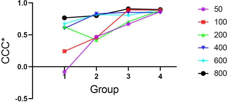
The distribution of CCC* among each group in six concentration sets.

Location-stability

After the Kruskal-Wallis test among four groups in each concentration test set, 23 qualified features with location-stability were selected. Their names and p-values in six concentration sets are shown in Table 4.

Table 4.

P value of qualified features in the Kruskal-Wallis test

Potentially Qualified Feature		Concentration(mg/mL)
		50	100	200	400	600	800
Intensity- Histogram	Skewness	0.069	<0.001	<0.001	<0.001	0.010	0.001
	Kurtosis	0.117	0.040	0.023	<0.001	<0.001	0.169
	Quartile Coefficient Of Dispersion	0.074	<0.001	0.008	<0.001	<0.001	<0.001
	Maximum Histogram Gradient	0.017	<0.001	0.009	0.157	<0.001	0.002
	Minimum Histogram Gradient	0.973	0.193	0.150	0.126	0.003	<0.001
GLCM	Joint Maximum	0.004	<0.001	0.002	<0.001	0.294	<0.001
	Normalized Inverse Difference	0.002	0.020	0.002	0.158	<0.001	<0.001
	Inverse Difference Moment	0.045	0.083	<0.001	<0.001	<0.001	<0.001
	Normalized Inverse Difference Moment	0.002	0.009	0.001	0.138	<0.001	<0.001
	Cluster Shade	0.133	<0.001	<0.001	<0.001	0.079	<0.001
GLRLM	Short Runs Emphasis	0.024	0.463	0.114	0.004	<0.001	<0.001
	Long Runs Emphasis	0.002	0.078	0.076	<0.001	<0.001	<0.001
	Grey Level Non-Uniformity	<0.001	<0.001	0.113	<0.001	<0.001	<0.001
	Run Percentage	0.010	0.225	0.074	0.002	<0.001	<0.001
NGTDM	Coarseness	<0.001	0.100	<0.001	0.623	<0.001	<0.001
	Busyness	<0.001	<0.001	0.084	0.049	<0.001	<0.001
GLSZM	Small Zone Emphasis	<0.001	0.067	0.001	<0.001	<0.001	<0.001
	Large Zone Emphasis	0.008	0.176	<0.001	0.006	<0.001	<0.001
	Grey Level Non-Uniformity	<0.001	<0.001	0.053	<0.001	<0.001	<0.001
	Normalized Zone Size Non-Uniformity	<0.001	0.104	0.002	<0.001	<0.001	<0.001
	Zone Percentage	0.207	0.143	0.001	0.002	<0.001	<0.001
	Zone Size Variance	<0.001	0.135	0.001	0.001	0.009	<0.001
	Zone Size Entropy	<0.001	<0.001	<0.001	0.060	<0.001	<0.001

There are significant differences in the number of qualified features for different concentrations. (Table 3) With the increase in concentration, the number of qualified features first increased and then decreased, and the numbers of qualified features in high-concentration sets were obviously less than those in low-concentration sets.

It was surprising that there was no consensus feature that was deemed qualified in both the reproducibility and location-stability experiments.

Discussion

High-throughput extraction of tissue and lesion features, quantitative analysis of data for diagnosis, ^23,24 monitoring disease progression, ^25,26 and predicting clinical endpoints ^27,28 are some applications of radiomics. As the basis of radiomic models, the characteristics of the features can eventually affect the reliability of the model output. In fact, after realizing the importance of feature screening, related research has been widely carried out on major imaging devices, including CT, ^29–31 PET, ³² MRI, ^33–36 and ultrasound. ^37,38 The increased and unevenly distributed confounding factors in CBCT images raised concerns about the reliability of extracted features. ^11–15 In this study, different concentrations of K₂HPO₄ aqueous solution were used to evaluate the reproducibility and location-stability of radiomic features.

In the past, a great deal of effort was made to evaluate feature reproducibility. Several studies indicated that the proportion of reproducible features may be related to equipment, ^39,40 acquisition parameters, ^39–43 image reconstruction, ^44,45 target region ²¹ etc. In our reproducibility experiment, we adopted the same parameter settings for test and retest sets and creatively incorporated concentration and spatial location into the study design.

To achieve this goal, we took the K₂HPO₄ aqueous solutions as the target object and manually set their spatial location in the FOV. Due to the similarity of K₂HPO₄’s effective atomic number to hydroxyapatite, it is frequently employed as a core material in liquid phantoms for simulating X-ray attenuation in bone. Unlike solid phantoms commonly used in CT radiomic studies, ^39,42 liquid phantoms can simulate X-ray attenuation at different densities by adjusting solution concentrations, allowing for experimental observations at various densities of the same object. As mentioned in Matheus Oliveira’s research, ¹⁴ K₂HPO₄ in the range from 50 to 800 mg ml⁻¹ of concentration can be equivalent to the attenuation of trabecular bone with varying degrees of mineralization.

The results showed some radiomic features that were not reproducible even with the same parameter settings, which is similar to some previous reproducibility studies. ^22,46–49 Moreover, the reproducibility of CBCT-derived features was density- and location-related. Specifically, the target object with a higher density or located in the peripheral area of the FOV had a higher number of reproducible features. Confounding imaging factors are partly responsible for this phenomenon due to their various spatial distribution and density dependence. Confounding factors, such as scatter radiation, might be higher in the center area of the FOV, as demonstrated in AK Hunter’s study. ⁵⁰ As for density, based on our results, it is reasonable to hypothesize that the influence of confounding factors in a low-density target might be more obvious than that in a high-density target.

This is probably the first study to assess the location-stability of radiomic features in the same FOV. Previous investigations were mainly focused on the location stability of grey values. Matheus Oliveira et al ¹⁴ demonstrated that the absolute CT numbers vary significantly with anatomical locations, using K₂HPO₄ solutions and a human skull phantom. Azin Parsa’s study showed similar results using a dry human mandible. ¹⁵ The shortcomings of CBCT grey value have been widely acknowledged. It is reasonable to doubt the stability of extracted radiomic features, especially the first-order features which directly reflect the grey value distribution. The results of our experiment confirmed our concern. Most of the features did not have location-stability in any concentration set, and none of the features had location-stability in all concentration sets. There were more location-stable features in low concentration sets. The confounding factors, such as beam hardening, ^51,52 which changes with the density of the target, might be responsible for this phenomenon. The non-monotonic variation in the number of qualified features (first increased and then decreased) may be attributed to the joint action of multiple confounding factors.

The current research has following limitations. First, all the experiments were conducted in a single CBCT equipment, which may limit the generalization of the findings. In addition, we used K₂HPO₄ solution as the reference, ignoring the effect of microstructure such as trabecular bone on ray scattering, which may make our results more optimistic. Finally, the experimental setting of the phantom smaller than FOV completely avoided the influence of exomass ^16,53 and may increase the number of qualified features.

The reliability of radiomic features extracted from CBCT images was not considered in previously related published data which applied this methodology. Our study demonstrated that the density and location of the target object can directly affect the reliability of the features. Meanwhile, the limitations of CBCT-derived features, such as lack of reproducibility or location-stability, or not having both at the same time, also greatly hampered their application scenarios. According to our study results, it is extremely recommended to clarify the priority of reproducibility or location-stability at the beginning in a CBCT-based radiomic research, so as to select appropriate radiomic features accordingly.

The study on radiomic features derived from CBCT is far from enough; therefore, more research needs to be carried out in a simulated clinical environment. In recent years, many methods have emerged to improve the quality of CBCT images, ^54–56 which may be a fundamental way to solve the problem of the features’ reliability and is also one of the directions of future research.

Conclusions

The reproducibility and location-stability of radiomic features derived from CBCT were assessed by a multiconcentration phantom. The density and location of the target object affected the reproducibility of features. Few features met the standard of location-stability, and the location-stability was affected by the density of the target object. When using CBCT as the research platform for radiomics, we should be cautious about the reliability of radiomic features.

REFERENCES

- 1. Lambin P, Rios-Velazquez E, Leijenaar R, Carvalho S, van Stiphout RGPM, Granton P, et al. Radiomics: extracting more information from medical images using advanced feature analysis. Eur J Cancer 2012; 48: 441–46. doi: 10.1016/j.ejca.2011.11.036 [DOI] [PMC free article] [PubMed] [Google Scholar]
- 2. Jiang ZY, Lan TJ, Cai WX, Tao Q. Primary clinical study of Radiomics for diagnosing simple bone Cyst of the jaw. Dentomaxillofac Radiol 2021; 50(): 20200384. doi: 10.1259/dmfr.20200384 [DOI] [PMC free article] [PubMed] [Google Scholar]
- 3. Yilmaz E, Kayikcioglu T, Kayipmaz S. Computer-aided diagnosis of periapical Cyst and Keratocystic Odontogenic tumor on cone beam computed tomography. Comput Methods Programs Biomed 2017; 146: 91–100. doi: 10.1016/j.cmpb.2017.05.012 [DOI] [PubMed] [Google Scholar]
- 4. Abdolali F, Zoroofi RA, Otake Y, Sato Y. Automated classification of Maxillofacial cysts in cone beam CT images using Contourlet transformation and spherical Harmonics. Comput Methods Programs Biomed 2017; 139: 197–207. doi: 10.1016/j.cmpb.2016.10.024 [DOI] [PubMed] [Google Scholar]
- 5. Bianchi J, Gonçalves JR, de Oliveira Ruellas AC, Ashman LM, Vimort J-B, Yatabe M, et al. Quantitative bone imaging biomarkers to diagnose Temporomandibular joint osteoarthritis. International Journal of Oral and Maxillofacial Surgery 2021; 50: 227–35. doi: 10.1016/j.ijom.2020.04.018 [DOI] [PMC free article] [PubMed] [Google Scholar]
- 6. Bianchi J, de Oliveira Ruellas AC, Gonçalves JR, Paniagua B, Prieto JC, Styner M, et al. Osteoarthritis of the Temporomandibular joint can be diagnosed earlier using biomarkers and machine learning. Sci Rep 2020; 10(. doi: 10.1038/s41598-020-64942-0 [DOI] [PMC free article] [PubMed] [Google Scholar]
- 7. Haghnegahdar AA, Kolahi S, Khojastepour L, Tajeripour F. Diagnosis of Tempromandibular disorders using local binary patterns. J Biomed Phys Eng 2018; 8: 87–96. [PMC free article] [PubMed] [Google Scholar]
- 8. De Rosa CS, Bergamini ML, Palmieri M, Sarmento DJ de S, de Carvalho MO, Ricardo ALF, et al. Differentiation of periapical Granuloma from Radicular Cyst using cone beam computed tomography images texture analysis. Heliyon 2020; 6: e05194. doi: 10.1016/j.heliyon.2020.e05194 [DOI] [PMC free article] [PubMed] [Google Scholar]
- 9. Okada K, Rysavy S, Flores A,Linguraru MG.. Noninvasive differential diagnosis of dental periapical lesions in cone-beam CT scans. Med Phys 2015; 42: 1653-1665. doi: 10.1118/1.4914418 [DOI] [PubMed] [Google Scholar]
- 10. Costa ALF, de Souza Carreira B, Fardim KAC, Nussi AD, da Silva Lima VC, Miguel MMV, et al. Texture analysis of cone beam computed tomography images reveals dental implant stability. Int J Oral Maxillofac Surg 2021; 50: 1609–16. doi: 10.1016/j.ijom.2021.04.009 [DOI] [PubMed] [Google Scholar]
- 11. Nishikawa K, Kousuge Y,Sano T.. Is application of a quantitative CT technique helpful for quantitative measurement of bone density using dental cone-beam CT? Oral Radiol 2016; 32: 9-13. doi: 10.1007/s11282-015-0202-z [DOI] [Google Scholar]
- 12. Pauwels R, Jacobs R, Singer SR, Mupparapu M. CBCT-based bone quality assessment: are Hounsfield units applicable Dentomaxillofacial Radiology 2015; 44: 20140238. doi: 10.1259/dmfr.20140238 [DOI] [PMC free article] [PubMed] [Google Scholar]
- 13. Kim D-G. Can dental cone beam computed tomography assess bone mineral density? J Bone Metab 2014; 21: 117–26. doi: 10.11005/jbm.2014.21.2.117 [DOI] [PMC free article] [PubMed] [Google Scholar]
- 14. Oliveira ML, Tosoni GM, Lindsey DH, Mendoza K, Tetradis S,Mallya SM.. Influence of anatomical location on CT numbers in cone beam computed tomography. Oral Surg Oral Med Oral Pathol Oral Radiol 2013; 115: 558-564. doi: 10.1016/j.oooo.2013.01.021 [DOI] [PubMed] [Google Scholar]
- 15. Parsa A, Ibrahim N, Hassan B, van der Stelt P, Wismeijer D. Influence of object location in cone beam computed tomography (Newtom 5G and 3d Accuitomo 170) on gray value measurements at an implant site. Oral Radiol 2014; 30: 153–59. doi: 10.1007/s11282-013-0157-x [DOI] [Google Scholar]
- 16. Candemil AP, Salmon B, Freitas DQ, Haiter-Neto F,Oliveira ML.. Distribution of metal artifacts arising from the exomass in small field-of-view cone beam computed tomography scans. Oral Surg Oral Med Oral Pathol Oral Radiol 2020; 130: 116-125. doi: 10.1016/j.oooo.2020.01.002 [DOI] [PubMed] [Google Scholar]
- 17. Nioche C, Orlhac F, Boughdad S, Reuze S, Goya-Outi J,Robert C, et al. LIFEx: A Freeware for Radiomic Feature Calculation in Multimodality Imaging to Accelerate Advances in the Characterization of Tumor Heterogeneity. Cancer Res 2018; 78: 4786-4789. doi: 10.1158/0008-5472.CAN-18-0125 [DOI] [PubMed] [Google Scholar]
- 18. Larue RTHM, van Timmeren JE, de Jong EEC, Feliciani G, Leijenaar RTH, Schreurs WMJ, et al. Influence of gray level Discretization on Radiomic feature stability for different CT scanners, tube currents and slice thicknesses: a comprehensive phantom study. Acta Oncol 2017; 56: 1544–53. doi: 10.1080/0284186X.2017.1351624 [DOI] [PubMed] [Google Scholar]
- 19. Orlhac F, Soussan M, Chouahnia K, Martinod E,Buvat I.. 18F-FDG PET-Derived Textural Indices Reflect Tissue-Specific Uptake Pattern in Non-Small Cell Lung Cancer. PLoS One 2015; 10: e145063. doi: 10.1371/journal.pone.0145063 [DOI] [PMC free article] [PubMed] [Google Scholar]
- 20. Lin LI. A Concordance correlation coefficient to evaluate reproducibility. Biometrics 1989; 45: 255–68. [PubMed] [Google Scholar]
- 21. Wang H, Zhou Y, Wang X, Zhang Y, Ma C, Liu B, et al. Reproducibility and Repeatability of CBCT-derived Radiomics features. Front Oncol 2021; 11: 773512. doi: 10.3389/fonc.2021.773512 [DOI] [PMC free article] [PubMed] [Google Scholar]
- 22. Fave X, Mackin D, Yang J, Zhang J, Fried D, Balter P, et al. Can Radiomics features be reproducibly measured from CBCT images for patients with non-small cell lung cancer Med Phys 2015; 42: 6784–97. doi: 10.1118/1.4934826 [DOI] [PMC free article] [PubMed] [Google Scholar]
- 23. Al Bulushi Y, Saint-Martin C, Muthukrishnan N, Maleki F, Reinhold C, Forghani R. Radiomics and machine learning for the diagnosis of pediatric Cervical non-tuberculous Mycobacterial Lymphadenitis. Sci Rep 2022; 12(): 2962. doi: 10.1038/s41598-022-06884-3 [DOI] [PMC free article] [PubMed] [Google Scholar]
- 24. Sun W, Liu S, Guo J, Liu S, Hao D, Hou F, et al. A CT-based Radiomics Nomogram for distinguishing between benign and malignant bone tumours. Cancer Imaging 2021; 21(): 20. doi: 10.1186/s40644-021-00387-6 [DOI] [PMC free article] [PubMed] [Google Scholar]
- 25. Sun R, Limkin EJ, Vakalopoulou M, Dercle L, Champiat S, Han SR, et al. A Radiomics approach to assess tumour-infiltrating Cd8 cells and response to anti-PD-1 or anti-PD-L1 Immunotherapy: an imaging biomarker, retrospective Multicohort study. Lancet Oncol 2018; 19: 1180–91. doi: 10.1016/S1470-2045(18)30413-3 [DOI] [PubMed] [Google Scholar]
- 26. Kim JY, Park JE, Jo Y, Shim WH, Nam SJ, Kim JH, et al. Incorporating Diffusion- and perfusion-weighted MRI into a Radiomics model improves diagnostic performance for Pseudoprogression in glioblastoma patients. Neuro Oncol 2019; 21: 404–14. doi: 10.1093/neuonc/noy133 [DOI] [PMC free article] [PubMed] [Google Scholar]
- 27. Li F, Pan D, He Y, Wu Y, Peng J, Li J, et al. Using ultrasound features and Radiomics analysis to predict lymph node metastasis in patients with thyroid cancer. BMC Surg 2020; 20(): 315. doi: 10.1186/s12893-020-00974-7 [DOI] [PMC free article] [PubMed] [Google Scholar]
- 28. Li G, Li L, Li Y, Qian Z, Wu F, He Y, et al. An MRI Radiomics approach to predict survival and tumour-infiltrating Macrophages in gliomas. Brain 2022; 145: 1151–61. doi: 10.1093/brain/awab340 [DOI] [PMC free article] [PubMed] [Google Scholar]
- 29. Berenguer R, Pastor-Juan MDR, Canales-Vázquez J, Castro-García M, Villas MV, Mansilla Legorburo F, et al. Radiomics of CT features may be Nonreproducible and redundant: influence of CT acquisition parameters. Radiology 2018; 288: 407–15. doi: 10.1148/radiol.2018172361 [DOI] [PubMed] [Google Scholar]
- 30. Meyer M, Ronald J, Vernuccio F, Nelson RC, Ramirez-Giraldo JC, Solomon J, et al. Reproducibility of CT Radiomic features within the same patient: influence of radiation dose and CT reconstruction settings. Radiology 2019; 293: 583–91. doi: 10.1148/radiol.2019190928 [DOI] [PMC free article] [PubMed] [Google Scholar]
- 31. Peng X, Yang S, Zhou L, Mei Y, Shi L, Zhang R, et al. Repeatability and reproducibility of computed tomography Radiomics for pulmonary nodules: A multicenter phantom study. Invest Radiol 2022; 57: 242–53. doi: 10.1097/RLI.0000000000000834 [DOI] [PMC free article] [PubMed] [Google Scholar]
- 32. Keller H, Shek T, Driscoll B, Xu Y, Nghiem B, Nehmeh S, et al. Noise-based image harmonization significantly increases Repeatability and reproducibility of Radiomics features in PET images: A phantom study. Tomography 2022; 8: 1113–28. doi: 10.3390/tomography8020091 [DOI] [PMC free article] [PubMed] [Google Scholar]
- 33. Wennmann M, Bauer F, Klein A, Chmelik J, Grözinger M, Rotkopf LT, et al. In vivo Repeatability and Multiscanner reproducibility of MRI Radiomics features in patients with Monoclonal plasma cell disorders: A prospective bi-institutional study. Invest Radiol 2023; 58: 253–64. doi: 10.1097/RLI.0000000000000927 [DOI] [PubMed] [Google Scholar]
- 34. Baeßler B, Weiss K, Pinto Dos Santos D. Robustness and reproducibility of Radiomics in magnetic resonance imaging: A phantom study. Invest Radiol 2019; 54: 221–28. doi: 10.1097/RLI.0000000000000530 [DOI] [PubMed] [Google Scholar]
- 35. Kim M, Jung SC, Park SY, Park BW, Choi KM. Impact of lesion size on reproducibility of quantitative measurement and Radiomic features in vessel wall MRI. Eur Radiol 2022; 33: 2195–2206. doi: 10.1007/s00330-022-09207-2 [DOI] [PubMed] [Google Scholar]
- 36. Carbonell G, Kennedy P, Bane O, Kirmani A, El Homsi M, Stocker D, et al. Precision of MRI Radiomics features in the liver and hepatocellular carcinoma. Eur Radiol 2022; 32: 2030–40. doi: 10.1007/s00330-021-08282-1 [DOI] [PubMed] [Google Scholar]
- 37. Li M-D, Cheng M-Q, Chen L-D, Hu H-T, Zhang J-C, Ruan S-M, et al. Reproducibility of Radiomics features from ultrasound images: influence of image acquisition and processing. Eur Radiol 2022; 32: 5843–51. doi: 10.1007/s00330-022-08662-1 [DOI] [PubMed] [Google Scholar]
- 38. Cobo T, Bonet-Carne E, Martínez-Terrón M, Perez-Moreno A, Elías N, Luque J, et al. Feasibility and reproducibility of fetal lung texture analysis by automatic quantitative ultrasound analysis and correlation with gestational age. Fetal Diagn Ther 2012; 31: 230–36. doi: 10.1159/000335349 [DOI] [PubMed] [Google Scholar]
- 39. Nardone V, Reginelli A, Guida C, Belfiore MP, Biondi M, Mormile M, et al. Delta-Radiomics increases Multicentre reproducibility: a phantom study. Med Oncol 2020; 37: 38. doi: 10.1007/s12032-020-01359-9 [DOI] [PubMed] [Google Scholar]
- 40. Varghese BA, Hwang D, Cen SY, Lei X, Levy J, Desai B, et al. Identification of robust and reproducible CT-texture Metrics using a customized 3d-printed texture phantom. J Appl Clin Med Phys 2021; 22: 98–107. doi: 10.1002/acm2.13162 [DOI] [PMC free article] [PubMed] [Google Scholar]
- 41. Biondi M, Vanzi E, De Otto G, Carbone SF, Nardone V, Banci Buonamici F. Effects of CT FOV displacement and acquisition parameters variation on texture analysis features. Phys Med Biol 2018; 63(): 235021. doi: 10.1088/1361-6560/aaefac [DOI] [PubMed] [Google Scholar]
- 42. Lu L, Liang Y, Schwartz LH,Zhao B.. Reliability of Radiomic Features Across Multiple Abdominal CT Image Acquisition Settings: A Pilot Study Using ACR CT Phantom. Tomography 2019; 5: 226-231. doi: 10.18383/j.tom.2019.00005 [DOI] [PMC free article] [PubMed] [Google Scholar]
- 43. Spuhler KD, Teruel JR, Galavis PE. Assessing the reproducibility of CBCT-derived Radiomics features using a novel three-dimensional printed phantom. Med Phys 2021; 48: 4326–33. doi: 10.1002/mp.15043 [DOI] [PubMed] [Google Scholar]
- 44. Zhao B, Tan Y, Tsai WY, Qi J, Xie C,Lu L, et al. Reproducibility of radiomics for deciphering tumor phenotype with imaging. Sci Rep 2016; 6: 23428. doi: 10.1038/srep23428 [DOI] [PMC free article] [PubMed] [Google Scholar]
- 45. Muenzfeld H, Nowak C, Riedlberger S, Hartenstein A, Hamm B,Jahnke P, et al. Intra-scanner repeatability of quantitative imaging features in a 3D printed semi-anthropomorphic CT phantom. Eur J Radiol 2021; 141: 109818. doi: 10.1016/j.ejrad.2021.109818 [DOI] [PubMed] [Google Scholar]
- 46. Balagurunathan Y, Kumar V, Gu Y, Kim J, Wang H, Liu Y, et al. Test-retest reproducibility analysis of lung CT image features. J Digit Imaging 2014; 27: 805–23. doi: 10.1007/s10278-014-9716-x [DOI] [PMC free article] [PubMed] [Google Scholar]
- 47. Hu P, Wang J, Zhong H, Zhou Z, Shen L, Hu W, et al. Reproducibility with repeat CT in Radiomics study for Rectal cancer. Oncotarget 2016; 7: 71440–46. doi: 10.18632/oncotarget.12199 [DOI] [PMC free article] [PubMed] [Google Scholar]
- 48. Caramella C, Allorant A, Orlhac F, Bidault F, Asselain B, Ammari S, et al. Can we trust the calculation of texture indices of CT images? A phantom study. Med Phys 2018; 45: 1529–36. doi: 10.1002/mp.12809 [DOI] [PubMed] [Google Scholar]
- 49. Delgadillo R, Spieler BO, Ford JC, Kwon D, Yang F, Studenski M, et al. Repeatability of CBCT Radiomic features and their correlation with CT Radiomic features for prostate cancer. Med Phys 2021; 48: 2386–99. doi: 10.1002/mp.14787 [DOI] [PubMed] [Google Scholar]
- 50. Hunter AK, McDavid WD. Characterization and correction of Cupping effect Artefacts in cone beam CT. Dentomaxillofac Radiol 2012; 41: 217–23. doi: 10.1259/dmfr/19015946 [DOI] [PMC free article] [PubMed] [Google Scholar]
- 51. Makins SR. Artifacts interfering with interpretation of cone beam computed tomography images. Dent Clin North Am 2014; 58: 485–95. doi: 10.1016/j.cden.2014.04.007 [DOI] [PubMed] [Google Scholar]
- 52. Molteni R. Prospects and challenges of rendering tissue density in Hounsfield units for cone beam computed tomography. Oral Surg Oral Med Oral Pathol Oral Radiol 2013; 116: 105–19. doi: 10.1016/j.oooo.2013.04.013 [DOI] [PubMed] [Google Scholar]
- 53. Araki K, Okano T. The effect of surrounding conditions on Pixel value of cone beam computed tomography. Clin Oral Implants Res 2013; 24: 862–65. doi: 10.1111/j.1600-0501.2011.02373.x [DOI] [PubMed] [Google Scholar]
- 54. Stankovic U, Ploeger LS, van Herk M, Sonke J-J. Optimal combination of anti-scatter Grids and software correction for CBCT imaging. Med Phys 2017; 44: 4437–51. doi: 10.1002/mp.12385 [DOI] [PubMed] [Google Scholar]
- 55. Rossi M, Belotti G, Paganelli C, Pella A, Barcellini A, Cerveri P, et al. Image‐Based shading correction for Narrow‐FOV TRUNCATED pelvic CBCT with deep Convolutional neural networks and transfer learning. Med Phys 2021; 48: 7112–26. doi: 10.1002/mp.15282 [DOI] [PMC free article] [PubMed] [Google Scholar]
- 56. Uneri A, Zhang X, Yi T, Stayman JW, Helm PA, Osgood GM, et al. Known-component metal Artifact reduction (KC-MAR) for cone-beam CT. Phys Med Biol 2019; 64(): 165021. doi: 10.1088/1361-6560/ab3036 [DOI] [PMC free article] [PubMed] [Google Scholar]
Associated Data
This section collects any data citations, data availability statements, or supplementary materials included in this article.