

Abstract
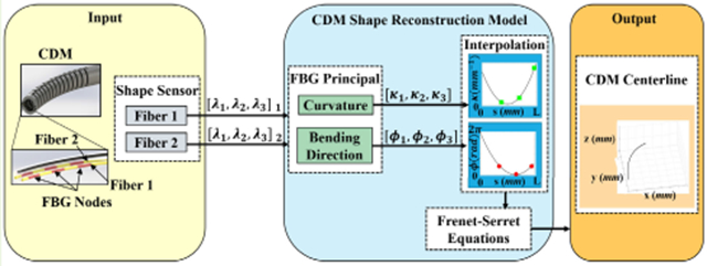
Continuum dexterous manipulators (CDMs) are suitable for performing tasks in a constrained environment due to their high dexterity and maneuverability. Despite the inherent advantages of CDMs in minimally invasive surgery, real-time control of CDMs’ shape during nonconstant curvature bending is still challenging. This study presents a novel approach for the design and fabrication of a large deflection fiber Bragg grating (FBG) shape sensor embedded within the lumens inside the walls of a CDM with a large instrument channel. The shape sensor consisted of two fibers, each with three FBG nodes. A shape-sensing model was introduced to reconstruct the centerline of the CDM based on FBG wavelengths. Different experiments, including shape sensor tests and CDM shape reconstruction tests, were conducted to assess the overall accuracy of the shape-sensing. The FBG sensor evaluation results revealed the linear curvature–wavelength relationship with the large curvature detection of 0.045 mm and a high wavelength shift of up to 5.50 nm at a 90° bending angle in both the bending directions. The CDM’s shape reconstruction experiments in a free environment demonstrated the shape-tracking accuracy of 0.216 ± 0.126 mm for positive/negative deflections. Also, the CDM shape reconstruction error for three cases of bending with obstacles was observed to be 0.436 ± 0.370 mm for the proximal case, 0.485 ± 0.418 mm for the middle case, and 0.312 ± 0.261 mm for the distal case. This study indicates the adequate performance of the FBG sensor and the effectiveness of the model for tracking the shape of the large-deflection CDM with nonconstant-curvature bending for minimally invasive orthopedic applications.
Keywords: Continuum manipulator, Fiber Bragg grating (FBG), large curvature, minimally invasive robotic surgery (MIRS), shape reconstruction, shape-sensing
Graphical Abstract
I. Introduction
IN RECENT years, continuum manipulators have shown great potential to improve steerability and dexterity in minimally invasive robotic surgery (MIRS) procedures. The compliant structure of continuum dexterous manipulators (CDMs) offers flexibility for reaching the targeted site of treatment in a constrained environment as their bodies can conform to their surroundings [1], [2], [3], [4], [5]. Despite many advantages of CDMs for medical applications, accurate estimation of its position and shape is a challenging task, especially when operating within unknown/unmodeled environments.
Approaches for the shape reconstruction of CDMs in surgical scenarios may include model-based, image-based, sensor-based, and/or their combination. The model-based approach uses the mechanics and kinematics of CDMs for shape reconstruction [6], [7], [8], [9], [10]. Due to the compliance of CDMs, these models may be complex and require a long computational time, making them challenging to use in real-time applications [6], [11]. The accuracy of the model-dependent CDM shape-sensing relies on the system parameter identification and assumptions when dealing with unknown disturbances and environmental constraints [12], [13]. The image-based approaches, on the other hand, may be more accurate since they do not rely on the mechanics of the CDM [14], [15]. However, radiation (i.e., fluoroscopy) or lower quality images (i.e., ultrasound imaging) introduce specific challenges for the real-time application of MIRS [16], [17].
The literature reports a number of shape-sensing approaches for real-time control and shape reconstruction of CDMs, including the use of piezoelectric polymers, electromagnetic (EM), and optical sensors [18], [19], [20]. EM and optical sensors are more commonly used, because of their smaller size, in real-time localization and the shape-tracking of CDMs for surgery [21], [22], [23]. EM tracking systems, however, are susceptible to errors arising from magnetic field distortions caused by the conductive objects in the work field [24].
The thin, flexible, lightweight, and biocompatible structure of optical shape sensors with the added advantage of EM immunity from external devices has received increasing attention in the sensor-based shape-sensing of the flexible instruments. By measuring the reflected wavelength from each fiber, strain and curvature sensing of FBG sensors enable accurate shape-tracking without relying on the kinematics and mechanics of the robotic systems [19], [25], [26], [27]. Optical fibers such as FBG with different configurations have been used for the shape reconstruction of flexible instruments such as catheters and biopsy needles as well as CDMs [28], [29], [30], [31]. FBG shape sensors, in particular, are classified into two main configurations: A bundle of single-core fibers and multicore fibers (MCFs). Roesthuis et al. [32] fabricated triplet optical fibers, each with four FBG nodes. Fibers were attached to a three-groove NiTi rod, placed in the backbone of the continuum manipulator. The 3-D shape of the manipulator has been reconstructed in terms of the curvature and strain relationship, derived from axial strain measurements of FBG nodes. Liu et al. [23] developed an FBG shape sensor by attaching a fiber with three FBG nodes to two NiTi rods in a triangular configuration and passing the sensor assembly through the sensor channel of a continuum manipulator. FBG wavelength–curvature calibration was used to find the curvature at discrete locations and then reconstruct the shape of the continuum manipulator. Sefati et al. [33] built an FBG sensor assembly by embedding a fiber and two NiTi rods into a three-lumen polycarbonate tube with circular cross section. The sensor assembly was passed through the side channel of a CDM. The design was later changed to insert three fibers, each with three FBG nodes, into the three-groove NiTi rod. A data-driven approach was developed to track the tip position of the CDM using FBG wavelength measurements [34], [35]. Moore and Rogge [36] reconstructed the 3-D shape using MCFs by combining the elastic rod theory and differential geometry. Khan et al. [37] used several MCFs for sensing the shape of a flexible medical instrument. The shape of the instrument is reconstructed using the curvature and torsion calculated from the FBG wavelength data. Cao et al. [38] integrated MCFs into a continuum robot to track the shape of the robot in the free space.
A major limitation of the previous work on the bundle of single-core fibers is the challenge and fabrication time associated with inserting and keeping fibers in the grooves of the sensor’s substrate due to the thin and delicate nature of fibers [28], [32], [34]. When the sensing unit is embedded into the channel within the wall of the continuum manipulator, the glue amount applied to the grooves of the sensor’s substrate is an important factor. Finding a sufficient amount of glue to not exceed the channel diameter constraint makes the building procedure difficult [32], [34]. Furthermore, attaching the fiber to the outer wall of the substrate is a complex manufacturing process. The sensor configuration becomes trial-dependent, making reproducibility a challenge [23]. The enclosed substrate is an appropriate option, especially if the sensor assembly is routed through the channels within the wall of the CDM. However, in the previous study, the shape sensor suffered from low sensitivity to small curvature changes, resulting in a low signal-to-noise ratio [33]. The shape sensor with MCFs, on the other hand, has a smaller cross section and more accurate FBG alignment [36], [37]. Nevertheless, light coupling into each core is difficult, and MCFs are more expensive than single-core fibers due to the draw tower fabrication procedure [39], [40]. Moreover, for applications in minimally invasive orthopedic interventions, a bundle of single-core fibers is sufficient for detecting the CDM centerline [23], [33], [34], [35]. Most of the prior work have introduced the FBG-based shape reconstruction algorithm for the case that the shape sensor is directly attached to the flexible medical instrument [26], [28], [32], [36], [37]. The free movement of the sensing unit inside the wall channel of the CDM makes shape-tracking difficult. The CDM centerline detection has rarely been developed in previous studies, and the sensing model did not account for the friction effect between the sensor and the CDM channel’s wall [23], [33], [34], [38].
The purpose of this study is to design and build a novel FBG-based shape sensor that is inexpensive and can be easily fabricated and integrated with a CDM undergoing large bending and deflections during orthopedic procedures. Another contribution includes the formulation of the shape reconstruction model for the CDM that can significantly lessen the influence of internal twist and friction. The performance of the model is assessed in both free and constrained environments.
II. Design
A. FBG Sensor Design Requirements
As shown in Fig. 1(a), the cable-driven CDM used in the orthopedic procedures has been constructed from a Nitinol (NiTi) rod with an outside diameter (OD) of 6 mm and several notches along its 35-mm flexible length to reach compliance in the bending direction while achieving high stiffness in the perpendicular direction to the bending plane [10]. The CDM also consists of a 4-mm-diameter open lumen as an instrument channel for passing flexible debriding tools [41] [Fig. 1(b)]. The overall length of the CDM is 70 mm, and the CDM wall contains four lengthwise channels such that each pair of channels is along the two opposite sides of the wall [Fig. 1(b)]. As shown in Fig. 1(c), the actuating cable is passed through its channel with a 0.5-mm diameter to create the bidirectional planar bending; the sensor channel with a diameter of 0.6 mm is for embedding the FBG-based shape-sensing unit into the CDM and tracking the 2-D-shape of the CDM in real-time [42].
Fig. 1.

(a) Schematics of the CDM while bending. (b) Cross section of the CDM tip, including sensor, cable, and instrument lengthwise channels. (c) Detailed view of the CDM flexible segment with the shape-sensing unit and the actuating cable.
The design requirements of the sensor assembly are derived from the CDM specifications and its applications. For orthopedic applications such as core decompression of the hip [41] and the treatment of osteolysis behind the acetabular implant [42], the outer diameter of the CDM must be less than 6 mm. The CDM has, therefore, a thin wall thickness (1 mm), with sensor channels of less than 0.5 mm [43]. Considering the major challenges of the previous work and CDM design constraints, the development of an FBG-based shape-sensing unit needs to meet some crucial requirements: 1)easy fabrication and integration into the CDM; 2)inexpensive compared to multicore optical fibers; 3)high wavelength-shift-to-curvature ratio (sensitivity) for small local deformations; 4) measure high deformations without surpassing the FBG strain limit; 5) less than 0.6-mm diameter to ensure easy sliding of the shape-sensing unit through the sensor channel; and 6) an enclosed structure to protect optical fibers and prevent adhesive wear due to the sensing unit slide inside the sensor channel.
B. FBG Sensor Configuration
The FBG-based shape sensor must undergo large bending and deflections with great elasticity. The Young’s modulus of the sensing unit’s substrate affects the position of the neutral plane of the sensor assembly; larger value of the Young’s modulus of the substrate increases its distance from the optical fibers. Furthermore, the substrate of the sensing unit needs to have an enclosed structure with smooth surface to avoid significant friction with the wall of the CDM’s sensor channel and hysteresis in the sensor assembly. To address the aforementioned requirements, a polycarbonate tube (shore hardness of 80) with an outer diameter of 500 ± 15 μm and three symmetric 150 ± 5 μm lumens was developed (Paradigm Optics, Inc.) [33]. Three lumens are 120° radially apart on a circle that has a 100-μm diameter. The three-lumen polycarbonate tube as a substrate meets requirements 1 and 5 to ensure simple sensor assembly, consistently repeatable fabrication, and unchallenging placement of the sensing unit into the CDM. The flexible enclosed structure of the polycarbonate tube fully covers optical fibers, which fulfills requirement 6. The strain of FBG fibers should not exceed their allowable range. The sensing unit can achieve high sensitivity and large deformations if the orthogonal distance between the FBG sensor and the neutral axis of the sensor assembly, called the sensor orthogonal distance, is neither too large nor too small [44], [45] (requirements 3 and 4). Hence, our sensing unit is designed with two optical fibers and one NiTi rod with a 125-μm diameter [Fig. 2(b)]. NiTi rod is chosen due to its super elastic property and the capability of undergoing large deflections. Also, the NiTi rod can increase the rigidity of the sensor assembly and, hence, its sensitivity. Plastic optical fibers have a thicker core diameter in the order of 1 mm compared with about 10-μm core diameter of silica optical fibers [46]. The much larger core diameter of plastic optical fibers provides high flexibility. However, the plastic optical fibers cannot be used as a component of the sensing unit due to the dimensional constraints of the CDM and the polycarbonate tube. A silica optical fiber with an 80-μm cladding diameter and a 120-μm polyimide coating diameter (Technica Optical Components, LLC., Atlanta, GA, USA) offers a small size for insertion into the three-lumen polycarbonate tube. The polyimide-coated fiber allows it to operate safely in the temperature range of −40 °C to +275 °C. The strain range of the optical fiber is up to 1.5%. Fig. 2(a) shows the arrangement of FBG nodes inside the CDM. The sensing unit is along the wall of the sensor channel which is doffset = 2.45 mm away from the CDM centerline. Since each fiber consists of three FBG nodes with a 5-mm length, the sensing unit includes three active areas () in total. is the FBG node on the fiber and is the active area. is the subscript that indicates the number associated with the active area and the corresponding FBG nodes. The center of the active areas are 10 mm apart, and the distance between the center of the active area and the distal end of the CDM is 5 mm. This arrangement of active areas provides adequate coverage for reconstructing the CDM centerline.
Fig. 2.

(a) Arrangement of FBG nodes, including two fibers and one NiTi rod, inside the CDM. Three sets of active areas along the length of the sensing unit are denoted by: , , and . (b) Shape-sensing unit in the cross section view. The two cores of fibers are labeled by Fiber 1 and Fiber 2.
For orthopedic applications, the FBG-sensorized CDM is chosen for some important reasons. Optical fibers are compatible to MRI-guided procedures because of the use of glass to transmit the light of specific wavelength as data [47]. In addition, optical fibers are suitable for real-time sensing applications due to the high acquisition frequency of up to 1 kHz [48].
C. Neutral Plane of the Sensing Unit
The neutral axis is normally positioned at the location of the geometric centroid. We assume that the sensing unit is a composite beam consisting of different materials at each cross section. As shown in Fig. 2(b), the sensing unit cross section is symmetric about the -axis of the local frame {n}, which is located at the center of the NiTi rod. Since the neutral plane always passes through the geometric centroid of the sensor assembly, , the y-coordinate of the geometric centroid is zero, , at each cross section. The z-coordinate of the geometric centroid, , can be derived from the equilibrium equation of forces in the local frame
| (1) |
where corresponds to the radius of the curvature. The subscript indicates the components of the sensing unit including the polycarbonate tube, NiTi rod, FBG fibers, and lumens of the polycarbonate tube. Also, , , and are the stress, Young’s modulus, and the cross section area of the component of the sensor assembly, respectively. Using (1), in the local frame can be obtained by
| (2) |
where components of the sensor assembly, namely, polycarbonate tube, NiTi rod, FBG fibers, and lumens of the polycarbonate tube are represented as subscripts , nw, , and , respectively. denotes the diameter of the sensor assembly component, and denotes the radius of the circle in which the center of three lumens of the polycarbonate tube is located. Young’s modulus of the polycarbonate tube, NiTi rod, and FBG fiber is 2.6, 75, and 70 GPa, respectively. By substituting the properties and dimensions of the sensor assembly components into (2), the value of becomes 0.095 mm. Changing the bending direction of the sensing unit affects the sensor’s orthogonal distance and hence the sensor sensitivity. To satisfy requirements 3 and 4 for both the optical fibers, the sensing unit’s neutral plane should be perpendicular to the CDM bending plane, making the sensor’s orthogonal distance to the two fibers equal.
D. Sensor Fabrication
1). FBG Sensor Assembly:
Since the core of the fiber alone is not affected by the bending strain, using the polycarbonate tube as a substrate can provide an offset between the center of the fiber and the neutral axis. Also, the fixed geometry of the three-lumen polycarbonate tube can help with the precise placement of sensor components. Two fibers were first passed through the two lumens while the tube was kept straight. After embedding and aligning both the fibers in the longitudinal direction of the tube, the UV glue (AA 3922, Loctite, Henkel), which has a low viscosity, was passed through the lumens by submerging one end in the UV glue and applying suction to the other end. The glue injection was continued until all the trapped air bubbles which are a potential source of the sensor error were removed. The NiTi rod was then passed through the third lumen, and finally, the UV glue inside the lumens was cured using a UV spot gun. Fig. 3(a) illustrates the segment of the shape-sensing unit after assembly. The new approach makes the sensor fabrication process far easier, less time-consuming (4 h of assembly), and low-cost (requirement 2) compared with previously reported designs [34], [37], [49].
Fig. 3.

(a) Section of the FBG sensor assembly. (b) FBG sensor assembly embedded in the CDM.
2). FBG Sensor Assembly Embedded in the CDM:
After assembly, as described in Section II-C, the sensing unit is passed through the CDM sensor channel such that its neutral plane is kept perpendicular to the CDM’s bending plane [Fig. 3(b)]. The sensor tip is then glued at the distal end of the CDM. The sensor, hence, can move freely as the CDM bends or straightens.
III. Methods
A. Principal of FBG-Based Shape-Sensing
The FBG wavelength shift is linearly dependent on the mechanical strain, , and the temperature, , which is given by [31], [50]
| (3) |
where is the FBG wavelength shift, and is the reference FBG wavelength at the reference strain, , and the reference temperature, . and refer to the constant coefficients associated with the strain and the temperature, respectively. The strain coefficient is directly related to the photo-elastic coefficient by , where the photo-elastic coefficient is set to 0.22 [51]. In this study, the reference wavelength is collected when the fiber is straight, and the reference strain, thus, can be assumed to be zero. Also, due to the proximity of fibers, the temperature variation in FBG nodes at each active area is the same [52]. In the case of the constant temperature, by measuring the FBG wavelength, strain can be calculated using (3).
B. Curvature Calculation of the Shape Sensor
The curvature and the bending direction of the shape sensor can be obtained by strain calculation at each active area, referred to as . Fig. 4 illustrates the cross section of the shape-sensing unit at . is the frame of the shape sensor centerline at the active area. The location of each active area and its associated strain, curvature, and bending direction are parameterized by the arc length, , which passes through the geometric centroid of the sensing unit. The arc length parameter is for reconstructing the shape sensor centerline. Axis is tangential to the shape sensor centerline, and the direction of the axis is from the origin of the frame to fiber 1 at the active area. Considering the pure bending for the sensing unit, equations which relate the axial strain, , of the FBG node on the fiber to the corresponding curvature and bending direction are as follows [32]:
| (4) |
| (5) |
where indicates the bending direction which is the angle between the axis of the local frame and the neutral axis. is the curvature, denotes the sensor orthogonal distance of the FBG node on the fiber, the radial distance from the FBG node on the fiber to the center of the polycarbonate tube, and is the angular offset from the negative axis to the core of the FBG node on the fiber.
Fig. 4.

Section of the shape-sensing unit at with the cross section view at FBG nodes labeled by and .
By assuming the reference strain to be zero, the following sets of equations can be derived from substituting (4) and (5) into (3):
| (6) |
| (7) |
where the term is the temperature variation at the active area. It is assumed that the term is the same for both the fibers due to the proximity of the FBG nodes at each active area. and are the wavelength shift and the reference wavelength associated with the FBG node on the fiber, respectively. Equations (6) and (7) can be simplified and then written in a matrix form
| (8) |
Where
from (8) can be obtained as
| (9) |
where is the Moore–Penrose pseudoinverse symbol. By solving (9), the curvature and the bending direction at the active area can be determined as
| (10) |
| (11) |
As shown in Fig. 5, the CDM can only bend in the plane of the planar bending which is aligned with the frame . is the frame of the CDM centerline at the proximal end of the CDM. Axis is tangential to the CDM centerline, and the direction of the axis is from the origin of the frame to the sensing unit. The wavelength shift sign of the sensing unit can simply specify the moving direction of the sensing unit and the CDM deflection direction; if the wavelength shifts of the FBG nodes on fiber 1 and fiber 2 are positive and negative, respectively, the CDM is undergoing positive deflection and the sensing unit is moving forward to the distal end of the CDM; if the situation is opposite, the CDM is undergoing negative deflection and the sensing unit is moving back to the proximal end of the CDM. Of note, the friction between the shape sensor and the wall of the CDM sensor channel affects the FBG wavelength measurements. To compensate for the influence of the friction, we consider a calibration coefficient at the active area, represented by
| (12) |
where is the compensated curvature at the active area after applying the calibration coefficient, and is the curvature at the active area before applying the calibration coefficient. Furthermore, the sensing unit may exhibit internal twists which result in the out-of-plane CDM centerline reconstruction. The effect of the twist on the bending direction is compensated at each active area by
| (13) |
where is the compensated bending direction at the active area, and is the twisted bending direction at the active area. Two steps are required to find as follows.
Fig. 5.

Moving direction of the shape-sensing unit at (a) CDM negative deflection and (b) CDM positive deflection. , , and are the initial locations of the active areas when the CDM is straight and , , and are the active areas locations after CDM bending.
The shape-sensing unit is lying straight in the plane of the bending plane such that the NiTi rod is facing the positive -direction. The wavelengths at each active area are recorded as the reference wavelength, .
The shape-sensing unit is inserted in a constant curvature groove which implies bending in the plane of the bending plane. Then, the twisted bending direction at each active area due to the internal twist can be computed using (9) and (11). These values are constant and do not change during the bending of the CDM, embedded with the sensing unit.
C. Sensor Assembly Shape Reconstruction
As described in Section III-B, the sensor assembly moves freely, while CDM bends (Fig. 5). Since the sliding amount of the sensing unit is unknown, the shape of the sensing unit is reconstructed from the distal end rather than the proximal end, where the arc lengths of all the active areas remain constant. As shown in Fig. 6, some coordinate systems are defined for reconstructing the shape sensor centerline. The measured FBG wavelengths are used to determine the curvature and the bending direction at the location of each active area, using (10)-(13). By knowing the arc length of each active area in frame as well as the corresponding curvature and bending direction, spline interpolation can be performed to compute the continuous curvature, , and the bending direction, . The interval of the arc length of the shape sensor centerline which is denoted by is from the origin of the frame to the last active area, .
Fig. 6.

Side cross section view of the CDM for shape reconstruction of the sensor assembly and the CDM. and are the frames of the shape sensor centerline at proximal and distal ends, respectively. Axes and are tangential to the curve of the shape sensor centerline. The direction of axes and is from the origin of their associated frames to fiber 2 and fiber 1, respectively.
As shown in Fig. 7, the centerline can be parameterized by the arc length as in the frame . Using the Frenet–Serret apparatus, the tangent of the curve, , is given by
| (14) |
where and represent the 2-D position of a point along the centerline in the frame . For the sensor assembly shape reconstruction, frame is considered as the frame . The slope of the centerline is related to the curvature by
| (15) |
where is the slope of the centerline which is the angle between the tangent vector at a point along the centerline and the positive direction of the -axis in the frame . is the initial value of the slope of the centerline at . By taking the integral of in (14), x- and y-positions of the centerline in terms of the arc length can be derived as
| (16) |
where and are the initial deflections in the x- and y-directions, respectively. Finally, the coordinates of the shape sensor centerline in the frame can be obtained using (15) and (16).
Fig. 7.

Centerline representation which is parameterized by a planar curve, , with Frenet–Serret vectors including the tangent vector, , and the normal vector, .
D. CDM Shape Reconstruction
The shape sensor centerline obtained in Section III-C should be translated to the CDM centerline, which has a constant offset, , from the shape sensor centerline (Fig. 6). and are the frames of the CDM centerline at the distal end and the corresponding cross section of the active area, respectively. Axes and are tangential to the curve of the CDM centerline. The direction of axes and are the same as axes and , respectively. The coordinate of the active area on the CDM centerline in the frame is determined by
| (17) |
where and denote the coordinates of the origin of the frame , and is a 3 × 3 rotation matrix about the z-axis from the frame to the frame by an angle . which is a 3 × 1 translation vector from the frame to the frame is found using (18)
| (18) |
where and are the coordinates of the active area on the shape sensor centerline. After finding the coordinates of active areas on the CDM centerline in the frame , it is possible to perform spline interpolation to find the arc length of each active area in the frame
| (19) |
where is the function associated with the fit curve of the CDM centerline in frame , denotes the arc length of the CDM centerline which its interval from the origin of the frame to the origin of the frame , and is the total arc length of the CDM centerline. Next, the curvature of each active area on the shape sensor centerline needs to be translated to the CDM centerline by
| (20) |
where is the curvature of the active area on the CDM centerline. Using (19) and (20), the continuous curvature of the CDM center curve, , can be determined by spline interpolation. Finally, considering the frame as the frame , and instead of , the coordinates of the CDM centerline can be found using (15) and (16).
IV. Experiments and Results
A. Experimental Setup
The experimental setup included actuation apparatus, the shape-sensing unit inside the CDM, and the stereo camera system (Fig. 8). The actuation apparatus consisted of the linear actuator for driving the actuating cable of the CDM, and a holding block to keep dc motors and the CDM’s chunk. The linear actuator consisted of two graphite brushed dc-motors (4.5W, RE 16, Maxon, Switzerland) with a high-precision encoder (MR, Type M, 512 CPT, Maxon, Switzerland) and an integrated gear box-ball screw mechanism (Spindle Drive GP 16S, Maxon, Switzerland), as well as a position controller (EPOS2, Maxon, Switzerland) [53]. While the CDM was bending, the FBG sensor wavelengths were measured by an optical sensing interrogator (sm130, Micron Optics Inc., Atlanta, GA) at a frequency of 100 Hz, which provides a wavelength resolution of 0.001 nm. Also, two FL2-08S2C cameras (Point Grey Research Inc., Richmond, BC, Canada), attached to the height-adjustable camera stand mount, captured the CDM images at a frequency of 30 Hz. To always make the CDM flexible segment visible to both the cameras, the cameras were placed 30 cm above the CDM working area. The measurements for FBG wavelengths were performed using a C++ code, developed using the C++ CISST-SAW libraries [54]. The images of both stereo cameras and FBG wavelengths were recorded, and (10)-(20) were applied to reconstruct the CDM centerline using the measured wavelengths.
Fig. 8.

Experimental setup, including the actuation apparatus, the stereo camera system, and the FBG shape sensor.
B. Image Processing
A pair of stereo cameras with a resolution of 1024 × 768 was used to track red markers attached to the CDM centerline. To find the cameras’ intrinsic and extrinsic matrices, the stereo camera pair was calibrated using the stereo camera calibration toolbox in MATLAB. The resulting overall mean error for the stereo pair calibration was 0.23 pixels. The measurement uncertainty of the stereo cameras after camera calibration was 0.253 mm, which was obtained by finding the Euclidean distance between two markers with predetermined positions on the calibration jig. The 3-D locations of the centroids of the markers were calculated by developing a computer algorithm for color-based segmentation and triangulation of the images (Fig. 9). The reconstructed CDM centerline from stereo images was then used as a ground truth to validate the CDM shape reconstruction model.
Fig. 9.

Extraction of 3-D locations of the CDM centerline from stereo images using color-based segmentation and triangulation.
C. Calibration
Two calibrations are needed to check the sensor manufacturing problems and conduct characterization process, one on the sensing unit alone and the second on the sensing unit inside the CDM. There exists a linear relationship between the change in FBG wavelength and its change in curvature [55]. To validate the linear relationship between the curvature and the FBG wavelength, 3-D-printed calibration jigs with discrete constant curvature grooves ranging from −90° to 90° at 5° interval and constant arc length were designed (Fig. 10). In this experiment, the sensing unit was examined at the optimal value of the sensor orthogonal distance, discussed in Section II-C. The sensing unit was fixed between two clamps to maintain the sensing unit’s orientation. Theoretically, the two fibers are symmetrical about the sensing unit’s central vertical plane, and hence the FBG wavelength shifts of each active area are almost similar at each curvature groove. The wavelengths of FBG nodes were sampled five times at each curvature groove, and then the mean value of data points was calculated. The sampling time was set to 3 s. Fig. 11 shows the linear fit between the wavelength shifts of three FBG nodes at each fiber and the changes in curvature. As shown in Fig. 12, the maximum standard deviation of data points is 0.146 nm. This indicates the high repeatability of results. The wavelength–curvature data points were well fit with lines, with R-squared (R2) in the range of 0.996–0.998.
Fig. 10.

Experimental setup for FBG sensors’ calibration using calibration jigs of positive and negative deflections with known curvatures.
Fig. 11.

Linear correlation between the curvature and wavelength of the shape-sensing unit at (a) fiber 1 and (b) fiber 2.
Fig. 12.

Standard deviation of data points related to the wavelength–curvature experiment of the shape-sensing unit at (a) fiber 1 and (b) fiber 2.
To accurately calculate the shape-sensing unit curvature and its bending direction from the FBG wavelength shifts, the distance of each FBG node from the center of the sensing unit and its orientation are required. Due to the manual fabrication of the sensing unit and the limited accuracy in the building process, the exact values of the position, , and orientation, , of each FBG node are unknown. For the characterization process, the data points of the wavelength–curvature experiment of the shape sensor for curvature grooves ranging from −90° to 90° at 10° interval were used. The predetermined constant, discrete curvature grooves, and their bending directions as well as the measured FBG wavelength shifts were used to find the position and orientation of each of FBG nodes. Considering the pure bending at a constant temperature, the calibration process at the active area was accomplished by a least-square optimization problem
| (21) |
where is the residual error of the observation, and is the set of unknown parameters for the positions and orientation of FBG nodes. is a stack of ground-truth data points for the curvature and bending direction, and is a stack of observation data points for the curvature and bending direction, obtained by (10) and (11). This minimization was implemented using least-squares method. The results are shown in Table I. To validate the accuracy of the obtained positions and orientations of FBG nodes, the data points of the wavelength–curvature experiment of the shape sensor for curvature grooves ranging from −85° to 85° at 10° interval were used. The results demonstrate that the model of the sensing unit with equivalent position and orientation of each FBG node can predict the curvature and bending direction with the mean error of 4.704e−4 ± 5.730e−4 mm−1 and 0.057° ± 0.019°, respectively.
TABLE I.
Calibrated Parameters for Positions (, , ) and Orientations (, , ) of FBG Nodes on Each Fiber ()
| Fiber index |
Position (mm) | Orientation (degree) | ||||
|---|---|---|---|---|---|---|
| 1 | 0.159 | 0.150 | 0.155 | 60.848 | 60.790 | 60.733 |
| 2 | 0.159 | 0.158 | 0.154 | 60.848 | 60.790 | 60.733 |
Based on the deflection direction and the inconsistent effect of the hindered friction at interactions between the sensing unit and the CDM sensor channel [56], the wavelength shifts at each active area for positive and negative deflections are not exactly the same. As discussed in Section II-B, two sets of calibration coefficients are defined at each active area; and are the calibration coefficients of the active area for positive and negative deflections, respectively. To obtain the calibration coefficients of the sensing unit inside the CDM, the effect of predetermined constant, discrete curvature grooves, and their bending directions on the FBG wavelength shifts for both the positive and negative deflections can be used. The 3D-printed calibration jigs with discrete curvature grooves ranging from −90° to 90° at 5° interval were designed (Fig. 13). The curvature and total arc length of each groove are constant. The CDM was fixed at its proximal end by two clamps, which were inserted into the slots of the stationary plate for maintaining the CDM’s bending plane parallel to the surface of the stationary plate. Five trials, one each with 3-s sampling time, were conducted at each groove. The wavelengths of FBG nodes from all the five trials were averaged. The standard deviation of data points is up to 0.169 nm which indicates the high repeatability of results. The calibration process was performed by a least-square optimization problem to find the set of coefficients that minimizes the curvature error at each active area. The experimental results of the CDM with embedded sensing unit for curvature grooves ranging from −90° to 90° at 10° interval were used for the least-square problem which is given by
| (22) |
where is the unknown coefficient of either or , based on the bending direction at the active area. is a stack of ground-truth data points for the curvature, and is a stack of observation data points for the curvature, obtained by (10) and (12). The results are shown in Table II.
Fig. 13.

Experimental setup for FBG sensors’ calibration inside the CDM using calibration jigs of positive and negative deflections with known curvatures.
TABLE II.
Calibration Coefficients for Positive (, , ) and Negative (, , ) Deflections of the Sensing Unit Inside the CDM ()
| Active area index |
Calibration coefficient | |
|---|---|---|
| 1 | 1.024 | 0.917 |
| 2 | 0.945 | 0.836 |
| 3 | 0.985 | 0.655 |
To find the accuracy of the obtained coefficients for curvature detection, the wavelength–curvature experimental results of the sensing unit inside the CDM for curvature grooves ranging from −85° to 85° at 10° interval were used. The results indicated that the model with the equivalent calibration coefficients can determine the curvature of positive and negative deflections with the mean error of 4.295e−4 ± 4.585e−4 mm−1 and 4.414e−4 ± 3.842e−4 mm−1, respectively. As discussed in Section III-B, the sign of the wavelength shifts at each active area can be used to specify the corresponding calibration coefficient of the model.
D. Static Experiment Conducted in Free Environment
Two sets of experiments in a free environment including positive and negative deflections were conducted. Each set of experiments consists of two cycles: bending and straightening. The bending cycle started from zero deflection at which the CDM was straight. Then, for each direction of deflection, the corresponding actuating cable was driven by the linear actuator, in the range of 0–5 mm, at 1-mm increments. When the actuating cable reached the maximum displacement, the straightening cycle was initiated such that the cable was released at 1-mm increments to return the CDM to its reference position. At each increment, the FBG wavelengths and the camera images of the CDM were recorded. Each set of experiments contains data points for nine cable displacements and repeated five times to assess the repeatability of the results.
The CDM’s centerlines obtained from the reconstruction model and stereo images are illustrated in Fig. 14. Each curve represents the average of five sampling data points. To compare the CDM centerlines with ground-truth data, the mean absolute error and standard deviation of the CDM centerline and tip pose in addition to the maximum absolute error of the CDM centerline were calculated at each cable displacement. The errors are presented in Table III. The results indicated a good agreement between the CDM centerline of the model and image in bending and straightening cycles with the overall mean error of 0.175 ± 0.081 mm for positive deflection, 0.262 ± 0.144 mm for negative deflection, and 0.216 ± 0.126 mm for positive/negative deflections. There was also a good agreement between the CDM tip pose of the model and image in bending and straightening cycles with the overall mean error of 0.197 ± 0.094 mm for positive deflection, 0.339 ± 0.202 mm for negative deflection, and 0.268 ± 0.172 mm for positive/negative deflections.
Fig. 14.

Shape reconstruction of the CDM in the free environment for (a) positive deflection and (b) negative deflection.
TABLE III.
Shape Reconstruction and Tip Position Errors of the CDM in the Free Environment
| Cycle | Cable displacement (mm) |
Positive deflection | Negative deflection | ||||||||
|---|---|---|---|---|---|---|---|---|---|---|---|
| Shape error | Tip error | Shape error | Tip error | ||||||||
| Mean (mm) |
Std. (mm) |
Max (mm) |
Mean (mm) |
Std. (mm) |
Mean (mm) |
Std. (mm) |
Max (mm) |
Mean (mm) |
Std. (mm) |
||
| Bending | 1 | 0.126 | 0.065 | 0.261 | 0.204 | 0.003 | 0.227 | 0.122 | 0.407 | 0.302 | 0.001 |
| 2 | 0.167 | 0.072 | 0.281 | 0.153 | 0.007 | 0.218 | 0.129 | 0.467 | 0.064 | 0.006 | |
| 3 | 0.163 | 0.063 | 0.280 | 0.211 | 0.028 | 0.252 | 0.118 | 0.488 | 0.201 | 0.014 | |
| 4 | 0.166 | 0.066 | 0.283 | 0.250 | 0.017 | 0.291 | 0.125 | 0.511 | 0.390 | 0.037 | |
| 5 | 0.191 | 0.077 | 0.305 | 0.249 | 0.019 | 0.357 | 0.159 | 0.617 | 0.559 | 0.110 | |
| Straightening | 4 | 0.271 | 0.071 | 0.292 | 0.187 | 0.003 | 0.296 | 0.190 | 0.656 | 0.656 | 0.004 |
| 3 | 0.139 | 0.064 | 0.276 | 0.188 | 0.009 | 0.214 | 0.093 | 0.386 | 0.213 | 0.003 | |
| 2 | 0.169 | 0.057 | 0.263 | 0.184 | 0.001 | 0.204 | 0.104 | 0.377 | 0.170 | 0.004 | |
| 1 | 0.142 | 0.008 | 0.267 | 0.185 | 0.004 | 0.210 | 0.105 | 0.361 | 0.238 | 0.003 | |
E. Static Experiment Conducted in Presence of Obstacles
To validate the shape reconstruction model in the case the contact forces applied along the CDM, two sets of experiments were conducted in the presence of obstacles for positive and negative deflections. As shown in Fig. 15, 3-D-printed obstacles were placed at three different locations along the length of the CDM which was: 1) near the proximal end; 2) in the middle segment; and 3) near the distal end.
Fig. 15.

Experimental setup of the CDM bending in constrained environment for (a)–(c) positive deflection and (d)–(f) negative deflection. Obstacles were placed at three different locations on each side of the CDM. (a) and (d) Proximal. (b) and (e) Middle. (c) and (f) Distal.
In each case, the segment of the CDM which interacted with the obstacle was obstructed from free bending and enforced the CDM to conform to more complex shapes. Each set of experiments was repeated five times. Fig. 16(a)-(c) and (d)-(f) shows the comparison between the ground-truth data extracted from stereo images and the reconstruction model in the constrained environment for positive and negative deflections, respectively. The mean absolute error and standard deviation of the CDM centerline and tip as well as the maximum absolute error of the CDM centerline for three obstacle-interaction cases are given in Table IV. The overall mean tracking accuracy of the CDM centerline for positive/negative deflections was 0.436 ± 0.370 mm, 0.485 ± 0.418 mm, and 0.312 ± 0.261 mm, respectively, for proximal, middle, and distal cases of CDM bending with obstacles. There was also a good accuracy between the CDM tip position derived from the model and image in positive/negative deflections with the overall mean error of 0.811 ± 0.383 mm for the proximal case, 1.040 ± 0.327 mm for the middle case, and 0.680 ± 0.422 mm for the distal case.
Fig. 16.

Shape reconstruction of the shape-sensing unit in the constrained environment for (a)–(c) positive deflection and (d)–(f) negative deflection in three different obstacle-interaction cases. (a) and (d) Proximal. (b) and (e) Middle. (c) and (f) Distal.
TABLE IV.
Shape Reconstruction and Tip Position Errors of the CDM in the Constrained Environment
| Obstacle status | Cable displacement (mm) |
Positive deflection | Negative deflection | ||||||||
|---|---|---|---|---|---|---|---|---|---|---|---|
| Shape error | Tip error | Shape error | Tip error | ||||||||
| Mean (mm) |
Std. (mm) |
Max (mm) |
Mean (mm) |
Std. (mm) |
Mean (mm) |
Std. (mm) |
Max (mm) |
Mean (mm) |
Std. (mm) |
||
| Proximal | 1 | 0.486 | 0.412 | 1.162 | 1.158 | 0.027 | 0.171 | 0.114 | 0.362 | 0.360 | 0.011 |
| 2 | 0.682 | 0.415 | 1.298 | 1.267 | 0.023 | 0.219 | 0.163 | 0.548 | 0.438 | 0.018 | |
| 3 | 0.753 | 0.436 | 1.477 | 1.321 | 0.108 | 0.210 | 0.121 | 0.539 | 0.478 | 0.038 | |
| 4 | 0.700 | 0.375 | 1.360 | 1.117 | 0.168 | 0.245 | 0.121 | 0.606 | 0.533 | 0.148 | |
| 5 | 0.620 | 0.337 | 1.264 | 0.996 | 0.277 | 0.276 | 0.161 | 0.812 | 0.547 | 0.217 | |
| Middle | 1 | 0.512 | 0.466 | 1.323 | 1.315 | 0.055 | 0.335 | 0.200 | 0.841 | 0.837 | 0.112 |
| 2 | 0.768 | 0.567 | 1.440 | 1.554 | 0.059 | 0.387 | 0.220 | 0.716 | 0.896 | 0.114 | |
| 3 | 0.675 | 0.401 | 1.256 | 1.157 | 0.074 | 0.275 | 0.254 | 0.820 | 0.798 | 0.107 | |
| 4 | 0.643 | 0.384 | 1.267 | 1.124 | 0.107 | 0.283 | 0.187 | 0.790 | 0.635 | 0.120 | |
| Distal | 1 | 0.235 | 0.144 | 0.617 | 0.614 | 0.012 | 0.391 | 0.167 | 0.542 | 0.540 | 0.011 |
| 2 | 0.479 | 0.328 | 1.210 | 1.199 | 0.019 | 0.242 | 0.175 | 0.274 | 0.366 | 0.021 | |
V. Discussion
This study presented a novel technique for building a thin, large deflection FBG-based shape-sensing unit that can be integrated into minimally invasive surgical systems. Our primary motivation is to develop a relatively inexpensive, easy-to-fabricate, and fast-fabricating (4 h versus days [34], [49]) shape-sensing for a CDM that is designed for orthopedic applications [43], [57]. The CDM, therefore, is constrained to bend in one plane and provide maximum stability and resistance to bending in the plane orthogonal to the bending plane. The proposed sensing method, however, can be extended to the CDM designs with 3-D bending. The shape reconstruction model was introduced to relate the wavelengths of FBG nodes to the curvature and bending direction of the CDM. The model was then implemented on the CDM, and its efficacy in free and constrained environments for positive and negative deflections was assessed.
The present technique for building the enclosed sensing unit was found to be easy, time-saving, repeatable, and cost-effective [37], [58]. The linear wavelength–curvature relationship of the developed shape-sensing unit (Fig. 11) had a pattern similar to previous studies [33], [34], [49], [55], [59]. For positive and negative deflections, the sensing unit has a high curvature sensitivity in terms of the wavelength shift, up to 124.875 nm·mm. Also, the FBG wavelength shift is up to 5.50 nm at the 90° bending angle compared with Sefati [34], up to 3 nm, and Liu [49], up to 4 nm. The resolution of the FBG shape sensor is calculated as 8.008e−6 mm−1, which is limited by the resolution of the optical sensing interrogator, 0.001 nm. The sensitivity-enhancing property enables the sensing unit to detect small changes in curvature. The maximum strain applied to the optical fiber at the 90° bending angle is 0.458%, which is still less than the strain range limit of the optical fiber. This implies that the FBG-based shape sensor can be safely used with a CDM undergoing large bending and deflections during orthopedic procedures.
The results of the static experiments in the free environment (Fig. 14 and Table III) and constrained environment (Fig. 16 and Table IV) indicate that the reconstruction model for tracking the CDM centerline is comprehensive and effective and justifies the building approach of the FBG-based shape-sensing unit used in our study. The reconstruction model could track the CDM centerline, which is extracted from stereo images, with a maximum shape deviation of 0.305 mm for positive deflection and 0.656 mm for negative deflection in the free environment (Table III), both below 2% of the CDM length, confirming the CDM is symmetric with respect to the deflection. The good consistency of the reconstruction model results in the constrained environment, implied by the maximum shape deviation of 1.477 mm for positive deflection and 0.841 mm for negative deflection (Table IV), suggests that the developed sensing unit and the reconstruction model are efficient for shape-tracking of the CDM, eliminating the need for integrated multicore optical fibers. Nevertheless, for the same actuating cable displacement, the mean errors of the CDM shape-tracking in obstacle-interaction cases were slightly higher than free bending. This may be due to the clearance between the sensing unit and the CDM sensor channel. Considering the free movement of the sensing unit inside the CDM sensor channel with its tip fixed at the distal end and the frictional effects within the channel, the rigor of the model was higher than the models developed for the sensing unit directly attached through the length of the medical instruments [26], [48], [60]. Moreover, compared with the data-driven approach which estimated the CDM centerline by solving a constrained optimization problem associated with the C-shaped bending [61], the proposed reconstruction model can be applied to S-shaped CDMs.
A limitation of the approach included the asymmetrical friction and local twist of the sensing unit affecting the shape reconstruction model by causing error in shape-sensing. Although these errors due to the free motion of the sensing unit inside the CDM sensor channel were reduced by applying the calibration coefficients, the small clearance between the sensing unit and the CDM sensor channel is still a source of error for the curvature estimation. Local twist measurement and incorporating its effects remain for the future studies. In addition, small errors in curvature estimation especially at the proximal end of the CDM can cause error accumulation through the CDM arclength. Depending on the accuracy requirements for a specified application, the number of FBG nodes at each shape-sensing unit and/or equipping the CDM with two shape sensors may improve the shape reconstruction model.
Hysteresis is another source of the error for CDM shape-tracking (Fig. 14). Hysteresis behavior in the CDM is due to factors including friction between the actuating cable and the CDM cable channel, backlash of the actuating cables, and the hysteresis property of the NiTi. The effect of hysteresis may require additional modeling and must be considered in the process of designing feedback control paradigms for the CDM.
In our study, the thermal conductivity of the NiTi rod used in the shape-sensing unit and the CDM body reduces the temperature gradient through the sensor length, which can decrease the influence of the temperature on the wavelength shifts of FBG nodes. Although this assumption in general is compatible with FBG-based shape sensors [38], if needed, the shape reconstruction model can be further extended to account for the changes in temperature.
VI. Conclusion
The goal of the study was to design, implement, and validate a novel shape reconstruction model, based on a CDM equipped with a novel FBG-based sensing unit developed in-house. The fabrication process of the FBG shape senor was easy and fast, using a polycabonate tube with three lumens as a flexible enclosed substrate. The sensing model accounted for the internal twist compensation and the hindered friction compensation between the sensing unit and the CDM sensor channel. To reconstruct the CDM centerline, the wavelength measurements of the FBG nodes were used to determine the curvature and bending direction of the CDM. The results of experiments demonstrated the linear wavelength–curvature relationship with high sensitivity and large bending capability. Moreover, it was shown in static experiments that the shape reconstruction model can accurately track the CDM centerline in free and constrained environments. It was concluded that the shape-sensing of the CDM in the presence of nonconstant curvature bending is feasible using the proposed sensing model.
Acknowledgment
The author would like to thank Dr. S. Sefati for his contribution with the development of the software infrastructure.
This work was supported in part by the National Institutes of Health (NIH) under Grant R01 EB016703 and Grant R01 AR080315. The associate editor coordinating the review of this article and approving it for publication was Prof. Arnaldo G. Leal-Junior.
Biographies

Golchehr Amirkhani received the B.Sc. degree in mechanical engineering from Shahid Beheshti University, Tehran, Iran, in 2015, and the M.Sc. degree in mechatronics from the Sharif University of Technology, Tehran, in 2018. She is currently pursuing the Ph.D. degree in mechanical engineering with Johns Hopkins University, Baltimore, MD, USA.
Her research interests include sensing and control of continuum manipulators with applications in surgical robotics and autonomous systems.

Anna Goodridge received the B.S. degree in mechanical engineering from Johns Hopkins University, Baltimore, MD, USA, in 2017.
She is currently working with the Laboratory for Computational Sensing and Robotics, Johns Hopkins University, as a Research Engineer. She has previously worked in research and development teams in the consumer product industry and her current work is with applications in surgical robotics and hardware design.

Mojtaba Esfandiari received the B.Sc. degree in mechanical engineering from the Amirkabir University of Technology (Tehran Polytechnic), Tehran, Iran, in 2014, and the M.Sc. degree in mechanical engineering from the Sharif University of Technology, Tehran, in 2017. He is currently pursuing the Ph.D. degree in mechanical engineering with Johns Hopkins University, Baltimore, MD, USA.
He was a Research Assistant at the Project neuroArm, University of Calgary, Calgary, AB, Canada, from 2018 to 2021. His research interests include modeling, optimization, and control of surgical robotic systems.

Henry Phalen (Graduate Student Member, IEEE) received the B.S. degree in bioengineering from the University of Pittsburgh, Pittsburgh, PA, USA, in 2018, and the M.S.E. degree in robotics from the Johns Hopkins University (JHU), Baltimore, MD, USA, in 2021, where he is currently pursuing the Ph.D. degree in mechanical engineering.
His research interests include state estimation and control of dexterous robotic systems in constrained and safety-critical environments with a focus on demonstrating integrated systems for use in surgical procedures.

Justin H. Ma (Graduate Student Member, IEEE) received the B.S. degree in mechanical engineering from the Georgia Institute of Technology, Atlanta, GA, USA, in 2019, and the M.S. degree in mechanical engineering from Johns Hopkins University, Baltimore, MD, USA, in 2022, where he is currently pursuing the Ph.D. degree in mechanical engineering.
His research interests include design and control of continuum manipulators and mechanisms for minimally invasive surgical robotics in orthopedics. He has previously worked in the medical device industry developing implants for spinal fusion.

Iulian Iordachita (Senior Member, IEEE) received the M.Eng. degree in industrial robotics and the Ph.D. degree in mechanical engineering from the University of Craiova, Craiova, Romania, in 1989 and 1996, respectively.
He is currently a Faculty Member with the Laboratory for Computational Sensing and Robotics, Johns Hopkins University, Baltimore, MD, USA, and the Director of the Advanced Medical Instrumentation and Robotics Research Laboratory. His current research interests include medical robotics, image-guided surgery, robotics, smart surgical tools, and medical instrumentation.

Mehran Armand (Member, IEEE) received the Ph.D. degree in mechanical engineering and kinesiology from the University of Waterloo, Waterloo, ON, Canada, in 1998.
He is currently a Professor of Orthopaedic Surgery, Mechanical Engineering, and Computer Science with Johns Hopkins University (JHU), Baltimore, MD, USA, and a Principal Scientist with the JHU Applied Physics Laboratory (JHU/APL). Prior to joining JHU/APL in 2000, he completed postdoctoral fellowship with the JHU Orthopaedic Surgery and Otolaryngology-Head and Neck Surgery. He currently directs the Laboratory for Biomechanical- and Image-Guided Surgical Systems, JHU Whiting School of Engineering. He also directs the AVICENNA Laboratory for advancing surgical technologies, Johns Hopkins Bayview Medical Center, Baltimore. His laboratory encompasses research in continuum manipulators, biomechanics, medical image analysis, and augmented reality for translation to clinical applications of integrated surgical systems in the areas of orthopedic, ENT, and craniofacial reconstructive surgery.
Contributor Information
Golchehr Amirkhani, Department of Mechanical Engineering and the Laboratory for Computational Sensing and Robotics, Johns Hopkins University, Baltimore, MD 21218 USA.
Anna Goodridge, Laboratory for Computational Sensing and Robotics, Johns Hopkins University, Baltimore, MD 21218 USA.
Mojtaba Esfandiari, Department of Mechanical Engineering and the Laboratory for Computational Sensing and Robotics, Johns Hopkins University, Baltimore, MD 21218 USA.
Henry Phalen, Department of Mechanical Engineering and the Laboratory for Computational Sensing and Robotics, Johns Hopkins University, Baltimore, MD 21218 USA.
Justin H. Ma, Department of Mechanical Engineering and the Laboratory for Computational Sensing and Robotics, Johns Hopkins University, Baltimore, MD 21218 USA.
Iulian Iordachita, Department of Mechanical Engineering and the Laboratory for Computational Sensing and Robotics, Johns Hopkins University, Baltimore, MD 21218 USA.
Mehran Armand, Department of Orthopedic Surgery, the Department of Mechanical Engineering, the Department of Computer Science, and the Laboratory for Computational Sensing and Robotics, Johns Hopkins University, Baltimore, MD 21218 USA.
References
- [1].Burgner-Kahrs J, Rucker DC, and Choset H, “Continuum robots for medical applications: A survey,” IEEE Trans. Robot, vol. 31, no. 6, pp. 1261–1280, Dec. 2015. [Google Scholar]
- [2].Simaan N, Taylor R, and Flint P, “High dexterity snake-like robotic slaves for minimally invasive telesurgery of the upper airway,” in Proc. Int. Conf. Med. Image Comput. Comput.-Assist. Intervent. Berlin, Germany: Springer, 2004, pp. 17–24. [Google Scholar]
- [3].Yip MC and Camarillo DB, “Model-less feedback control of continuum manipulators in constrained environments,” IEEE Trans. Robot, vol. 30, no. 4, pp. 880–889, Aug. 2014. [Google Scholar]
- [4].Vitiello V, Lee S-L, Cundy TP, and Yang G-Z, “Emerging robotic platforms for minimally invasive surgery,” IEEE Rev. Biomed. Eng, vol. 6, pp. 111–126, 2012. [DOI] [PubMed] [Google Scholar]
- [5].Amirkhani G, Farahmand F, Yazdian SM, and Mirbagheri A, “An extended algorithm for autonomous grasping of soft tissues during robotic surgery,” Int. J. Med. Robot. Comput. Assist. Surg, vol. 16, no. 5, pp. 1–15, Oct. 2020. [DOI] [PubMed] [Google Scholar]
- [6].Gao A, Murphy RJ, Liu H, Iordachita II, and Armand M, “Mechanical model of dexterous continuum manipulators with compliant joints and tendon/external force interactions,” IEEE/ASME Trans. Mechatronics, vol. 22, no. 1, pp. 465–475, Feb. 2017. [DOI] [PMC free article] [PubMed] [Google Scholar]
- [7].Rucker DC and Webster III RJ, “Statics and dynamics of continuum robots with general tendon routing and external loading,” IEEE Trans. Robot, vol. 27, no. 6, pp. 1033–1044, Dec. 2011. [Google Scholar]
- [8].Xu K and Simaan N, “Analytic formulation for kinematics, statics, and shape restoration of multibackbone continuum robots via elliptic integrals,” J. Mech. Robot, vol. 2, no. 1, 2010, Art. no. 011006. [Google Scholar]
- [9].Segreti SM, Kutzer MDM, Murphy RJ, and Armand M, “Cable length estimation for a compliant surgical manipulator,” in Proc. IEEE Int. Conf. Robot. Autom., May 2012, pp. 701–708. [Google Scholar]
- [10].Murphy RJ, Kutzer MDM, Segreti SM, Lucas BC, and Armand M, “Design and kinematic characterization of a surgical manipulator with a focus on treating osteolysis,” Robotica, vol. 32, no. 6, pp. 835–850, Sep. 2014. [Google Scholar]
- [11].Chirikjian GS, “Conformational modeling of continuum structures in robotics and structural biology: A review,” Adv. Robot, vol. 29, no. 13, pp. 817–829, Jul. 2015. [DOI] [PMC free article] [PubMed] [Google Scholar]
- [12].Webster RJ and Jones BA, “Design and kinematic modeling of constant curvature continuum robots: A review,” Int. J. Robot. Res, vol. 29, no. 13, pp. 1661–1683, Nov. 2010. [Google Scholar]
- [13].Moses MS, Murphy RJ, Kutzer MDM, and Armand M, “Modeling cable and guide channel interaction in a high-strength cable-driven continuum manipulator,” IEEE/ASME Trans. Mechatronics, vol. 20, no. 6, pp. 2876–2889, Dec. 2015. [DOI] [PMC free article] [PubMed] [Google Scholar]
- [14].Vandini A, Bergeles C, Lin F-Y, and Yang G-Z, “Vision-based intraoperative shape sensing of concentric tube robots,” in Proc. IEEE/RSJ Int. Conf. Intell. Robots Syst. (IROS), Sep. 2015, pp. 2603–2610. [Google Scholar]
- [15].Hannan MW and Walker ID, “Real-time shape estimation for continuum robots using vision,” Robotica, vol. 23, no. 5, pp. 645–651, Sep. 2005. [Google Scholar]
- [16].Lobaton EJ, Fu J, Torres LG, and Alterovitz R, “Continuous shape estimation of continuum robots using X-ray images,” in Proc. IEEE Int. Conf. Robot. Autom., May 2013, pp. 725–732. [DOI] [PMC free article] [PubMed] [Google Scholar]
- [17].Camarillo DB, Loewke KE, Carlson CR, and Salisbury JK, “Vision based 3-D shape sensing of flexible manipulators,” in Proc. IEEE Int. Conf. Robot. Autom., May 2008, pp. 2940–2947. [Google Scholar]
- [18].Sadjadi H, Hashtrudi-Zaad K, and Fichtinger G, “Simultaneous localization and calibration for electromagnetic tracking systems,” Int. J. Med. Robot. Comput. Assist. Surg, vol. 12, no. 2, pp. 189–198, Jun. 2016. [DOI] [PubMed] [Google Scholar]
- [19].Hill KO and Meltz G, “Fiber Bragg grating technology fundamentals and overview,” J. Lightw. Technol, vol. 15, no. 8, pp. 1263–1276, Aug. 1997. [Google Scholar]
- [20].Cianchetti M, Renda F, Licofonte A, and Laschi C, “Sensorization of continuum soft robots for reconstructing their spatial configuration,” in Proc. 4th IEEE RAS EMBS Int. Conf. Biomed. Robot. Biomechatronics (BioRob), Jun. 2012, pp. 634–639. [Google Scholar]
- [21].Feuerstein M, Reichl T, Vogel J, Traub J, and Navab N, “Magnetooptical tracking of flexible laparoscopic ultrasound: Model-based online detection and correction of magnetic tracking errors,” IEEE Trans. Med. Imag, vol. 28, no. 6, pp. 951–967, Jun. 2009. [DOI] [PubMed] [Google Scholar]
- [22].Ryu SC and Dupont PE, “FBG-based shape sensing tubes for continuum robots,” in Proc. IEEE Int. Conf. Robot. Automat. (ICRA), May 2014, pp. 3531–3537. [Google Scholar]
- [23].Liu H et al. , “Shape tracking of a dexterous continuum manipulator utilizing two large deflection shape sensors,” IEEE Sensors J, vol. 15, no. 10, pp. 5494–5503, Oct. 2015. [DOI] [PMC free article] [PubMed] [Google Scholar]
- [24].Franz AM, Haidegger T, Birkfellner W, Cleary K, Peters TM, and Maier-Hein L, “Electromagnetic tracking in medicine—A review of technology, validation, and applications,” IEEE Trans. Med. Imag, vol. 33, no. 8, pp. 1702–1725, Aug. 2014. [DOI] [PubMed] [Google Scholar]
- [25].Taffoni F, Formica D, Saccomandi P, Pino G, and Schena E, “Optical fiber-based MR-compatible sensors for medical applications: An overview,” Sensors, vol. 13, no. 10, pp. 14105–14120, Oct. 2013. [DOI] [PMC free article] [PubMed] [Google Scholar]
- [26].Khan F, Donder A, Galvan S, Baena FRY, and Misra S, “Pose measurement of flexible medical instruments using fiber Bragg gratings in multi-core fiber,” IEEE Sensors J, vol. 20, no. 18, pp. 10955–10962, Sep. 2020. [Google Scholar]
- [27].Abushagur A, Arsad N, Reaz M, and Bakar A, “Advances in biotactile sensors for minimally invasive surgery using the fibre Bragg grating force sensor technique: A survey,” Sensors, vol. 14, no. 4, pp. 6633–6665, Apr. 2014. [DOI] [PMC free article] [PubMed] [Google Scholar]
- [28].Park Y-L et al. , “Real-time estimation of 3-D needle shape and deflection for MRI-guided interventions,” IEEE/ASME Trans. Mechatronics, vol. 15, no. 6, pp. 906–915, Dec. 2010. [DOI] [PMC free article] [PubMed] [Google Scholar]
- [29].Farvardin A, Murphy RJ, Grupp RB, Iordachita I, and Armand M, “Towards real-time shape sensing of continuum manipulators utilizing fiber Bragg grating sensors,” in Proc. 6th IEEE Int. Conf. Biomed. Robot. Biomechatronics (BioRob), Jun. 2016, pp. 1180–1185. [Google Scholar]
- [30].Khan F, Roesthuis RJ, and Misra S, “Force sensing in continuum manipulators using fiber Bragg grating sensors,” in Proc. IEEE/RSJ Int. Conf. Intell. Robots Syst. (IROS), Sep. 2017, pp. 2531–2536. [Google Scholar]
- [31].Abayazid M, Kemp M, and Misra S, “3D flexible needle steering in soft-tissue phantoms using fiber Bragg grating sensors,” in Proc. IEEE Int. Conf. Robot. Autom., May 2013, pp. 5843–5849. [Google Scholar]
- [32].Roesthuis RJ, Janssen S, and Misra S, “On using an array of fiber Bragg grating sensors for closed-loop control of flexible minimally invasive surgical instruments,” in Proc. IEEE/RSJ Int. Conf. Intell. Robots Syst., Nov. 2013, pp. 2545–2551. [Google Scholar]
- [33].Sefati S, Alambeigi F, Iordachita I, Armand M, Murphy RJ, and Armand M, “FBG-based large deflection shape sensing of a continuum manipulator: Manufacturing optimization,” in Proc. IEEE SENSORS, Oct. 2016, pp. 1–3. [Google Scholar]
- [34].Sefati S, Pozin M, Alambeigi F, Iordachita I, Taylor RH, and Armand M, “A highly sensitive fiber Bragg grating shape sensor for continuum manipulators with large deflections,” in Proc. IEEE SENSORS, Oct. 2017, pp. 1–3.29780437 [Google Scholar]
- [35].Sefati S, Hegeman R, Alambeigi F, Iordachita I, and Armand M, “FBG-based position estimation of highly deformable continuum manipulators: Model-dependent vs. data-driven approaches,” in Proc. Int. Symp. Med. Robot. (ISMR), Apr. 2019, pp. 1–6. [Google Scholar]
- [36].Moore JP and Rogge MD, “Shape sensing using multi-core fiber optic cable and parametric curve solutions,” Opt. Exp, vol. 20, no. 3, pp. 2967–2973, 2012. [DOI] [PubMed] [Google Scholar]
- [37].Khan F, Denasi A, Barrera D, Madrigal J, Sales S, and Misra S, “Multi-core optical fibers with Bragg gratings as shape sensor for flexible medical instruments,” IEEE Sensors J, vol. 19, no. 14, pp. 5878–5884, Jul. 2019. [Google Scholar]
- [38].Cao Y, Liu Z, Yu H, Hong W, and Xie L, “Spatial shape sensing of a multisection continuum robot with integrated DTG sensor for maxillary sinus surgery,” IEEE/ASME Trans. Mechatronics, vol. 28, no. 2, pp. 715–725, Apr. 2023. [Google Scholar]
- [39].Takenaga K, Tanigawa S, Guan N, Matsuo S, Saitoh K, and Koshiba M, “Reduction of crosstalk by quasi-homogeneous solid multi-core fiber,” in Proc. Opt. Fiber Commun. Conf., 2010, pp. 1–3, Paper OWK7. [Google Scholar]
- [40].Flockhart GMH, MacPherson WN, Barton JS, Jones JDC, Zhang L, and Bennion I, “Two-axis bend measurement with Bragg gratings in multicore optical fiber,” Opt. Lett, vol. 28, no. 6, pp. 387–389, Mar. 2003. [DOI] [PubMed] [Google Scholar]
- [41].Alambeigi F et al. , “A curved-drilling approach in core decompression of the femoral head osteonecrosis using a continuum manipulator,” IEEE Robot. Autom. Lett, vol. 2, no. 3, pp. 1480–1487, Jul. 2017. [Google Scholar]
- [42].Sefati S et al. , “A surgical robotic system for treatment of pelvic osteolysis using an FBG-equipped continuum manipulator and flexible instruments,” IEEE/ASME Trans. Mechatronics, vol. 26, no. 1, pp. 369–380, Feb. 2021. [DOI] [PMC free article] [PubMed] [Google Scholar]
- [43].Sefati S, Hegeman R, Iordachita I, Taylor RH, and Armand M, “A dexterous robotic system for autonomous debridement of osteolytic bone lesions in confined spaces: Human cadaver studies,” IEEE Trans. Robot, vol. 38, no. 2, pp. 1213–1229, Apr. 2022. [DOI] [PMC free article] [PubMed] [Google Scholar]
- [44].Jang M, Kim JS, Um SH, Yang S, and Kim J, “Ultra-high curvature sensors for multi-bend structures using fiber Bragg gratings,” Opt. Exp, vol. 27, no. 3, pp. 2074–2084. Feb. 2019. [DOI] [PubMed] [Google Scholar]
- [45].Ge J, James AE, Xu L, Chen Y, Kwok K-W, and Fok MP, “Bidirectional soft silicone curvature sensor based on off-centered embedded fiber Bragg grating,” IEEE Photon. Technol. Lett, vol. 28, no. 20, pp. 2237–2240, Oct. 15, 2016. [Google Scholar]
- [46].Bhowmik K and Peng G-D, “Polymer optical fibers,” in Handbook of Optical Fibers. Singapore: Springer, 2019, pp. 1–51. [Google Scholar]
- [47].Henken KR, Dankelman J, van den Dobbelsteen JJ, Cheng LK, and van der Heiden MS, “Error analysis of FBG-based shape sensors for medical needle tracking,” IEEE/ASME Trans. Mechatronics, vol. 19, no. 5, pp. 1523–1531, Oct. 2014. [Google Scholar]
- [48].Al-Ahmad O, Ourak M, Van Roosbroeck J, Vlekken J, and Poorten EV, “Improved FBG-based shape sensing methods for vascular catheterization treatment,” IEEE Robot. Autom. Lett, vol. 5, no. 3, pp. 4687–4694, Jul. 2020. [Google Scholar]
- [49].Liu H, Farvardin A, Pedram SA, Iordachita I, Taylor RH, and Armand M, “Large deflection shape sensing of a continuum manipulator for minimally-invasive surgery,” in Proc. IEEE Int. Conf. Robot. Autom. (ICRA), May 2015, pp. 201–206. [DOI] [PMC free article] [PubMed] [Google Scholar]
- [50].Roesthuis RJ, Kemp M, van den Dobbelsteen JJ, and Misra S, “Three-dimensional needle shape reconstruction using an array of fiber Bragg grating sensors,” IEEE/ASME Trans. Mechatronics, vol. 19, no. 4, pp. 1115–1126, Aug. 2014. [Google Scholar]
- [51].Li R, Chen Y, Tan Y, Zhou Z, Li T, and Mao J, “Sensitivity enhancement of FBG-based strain sensor,” Sensors, vol. 18, no. 5, p. 1607, May 2018. [DOI] [PMC free article] [PubMed] [Google Scholar]
- [52].Xiong L, Jiang G, Guo Y, Kuang Y, and Liu H, “Investigation of the temperature compensation of FBGs encapsulated with different methods and subjected to different temperature change rates,” J. Lightw. Technol, vol. 37, no. 3, pp. 917–926, Feb. 1, 2019. [Google Scholar]
- [53].Ma JH, Sefati S, Taylor RH, and Armand M, “An active steering hand-held robotic system for minimally invasive orthopaedic surgery using a continuum manipulator,” IEEE Robot. Autom. Lett, vol. 6, no. 2, pp. 1622–1629, Apr. 2021. [DOI] [PMC free article] [PubMed] [Google Scholar]
- [54].Kazanzides P, Chen Z, Deguet A, Fischer GS, Taylor RH, and DiMaio SP, “An open-source research kit for the da Vinci surgical system,” in Proc. IEEE Int. Conf. Robot. Autom. (ICRA), May 2014, pp. 6434–6439. [Google Scholar]
- [55].Song K, Lezcano DA, Sun G, Kim JS, and Iordachita II, “Towards automatic robotic calibration system for flexible needles with FBG sensors,” in Proc. Int. Symp. Med. Robot. (ISMR), Nov. 2021, pp. 1–7. [DOI] [PMC free article] [PubMed] [Google Scholar]
- [56].Gao A, Zou Y, Wang Z, and Liu H, “A general friction model of discrete interactions for tendon actuated dexterous manipulators,” J. Mech. Robot, vol. 9, no. 4, 2017, Art. no. 041019. [Google Scholar]
- [57].Alambeigi F et al. , “On the use of a continuum manipulator and a bendable medical screw for minimally invasive interventions in orthopedic surgery,” IEEE Trans. Med. Robot. Bionics, vol. 1, no. 1, pp. 14–21, Feb. 2019. [DOI] [PMC free article] [PubMed] [Google Scholar]
- [58].Moon H, Jeong J, Kang S, Kim K, Song Y-W, and Kim J, “Fiber-Bragg-grating-based ultrathin shape sensors displaying single-channel sweeping for minimally invasive surgery,” Opt. Lasers Eng, vol. 59, pp. 50–55, Aug. 2014. [Google Scholar]
- [59].Kim JS, Guo J, Chatrasingh M, Kim S, and Iordachita I, “Shape determination during needle insertion with curvature measurements,” in Proc. IEEE/RSJ Int. Conf. Intell. Robots Syst. (IROS), Sep. 2017, pp. 201–208. [Google Scholar]
- [60].Donder A and Baena FRY, “Kalman-filter-based, dynamic 3-D shape reconstruction for steerable needles with fiber Bragg gratings in multicore fibers,” IEEE Trans. Robot, vol. 38, no. 4, pp. 2262–2275, Aug. 2022. [Google Scholar]
- [61].Sefati S, Gao C, Iordachita I, Taylor RH, and Armand M, “Data-driven shape sensing of a surgical continuum manipulator using an uncalibrated fiber Bragg grating sensor,” IEEE Sensors J, vol. 21, no. 3, pp. 3066–3076, Feb. 2021. [DOI] [PMC free article] [PubMed] [Google Scholar]