Super-resolution segmentation network for inner-ear tissue segmentation

Abstract

Cochlear implants (CIs) are considered the standard-of-care treatment for profound sensory-based hearing loss. Several groups have proposed computational models of the cochlea in order to study the neural activation patterns in response to CI stimulation. However, most of the current implementations either rely on high-resolution histological images that cannot be customized for CI users or CT images that lack the spatial resolution to show cochlear structures. In this work, we propose to use a deep learning-based method to obtain μCT level tissue labels using patient CT images. Experiments showed that the proposed super-resolution segmentation architecture achieved very good performance on the inner-ear tissue segmentation. Our best-performing model (0.871) outperformed the UNet (0.746), VNet (0.853), nnUNet (0.861), TransUNet (0.848), and SRGAN (0.780) in terms of mean dice score.

1. Introduction

Cochlear implants (CIs) are considered the standard-of-care treatment for profound sensory-based hearing loss. With over 700,000 recipients worldwide [15], CI is undoubtedly one of the most successful neural prostheses in history. Several groups have proposed computational models of the cochlea in order to simulate the neural activation patterns in response to CI stimulation, which can provide objective information for CI programming. Noble et al. proposed image-guided CI programming (IGCIP) techniques where CT-based intra-cochlear segmentation is used to estimate the electro-neural interface [18]. Although experiments have shown that IGCIP significantly improves hearing outcomes in clinical settings [16, 17], it estimates the neural response in a relatively coarse manner where only the spatial relationship between CI electrodes and neural sites is used. Frijns et al. proposed a rotationally symmetric model of cochlea [6] and Kalkman et al. proposed an electro-anatomical model (EAM) where a tissue label map of the inner ear is generated [11], they used boundary element method to solve for the voltage distribution in the electrically stimulated cochlea. Whiten et al. also created an EAM model of human cochlea, while they used the finite difference method to solve for the electric potential distribution [24]. Although these methods are useful to explore the mechanics of CI and neural response, they rely on 3D tissue electrical resistivity maps built based on histological images and cannot be applied in-vivo or customized for CI implant users. Malherbe et al. used patient specific EAMs based on CT images [14]. However, their method relies on manual point selection in CT images that don’t have fine enough resolution to show intra-cochlear structures. To overcome this, Cakir et al. developed an approach to create a high resolution patient-specific class map using multi-atlas segmentation, where μCTs with manual tissue class labels are non-rigidly registered to the patient CT [2]. The registration is done with a thin plate spline transformation that uses points in an active-shape-model based segmentation of the scalae structures as landmarks. As these landmarks are on the cochlear surface, the classification of tissues distant from the cochlea tends to not be very accurate, however, accurate labels are critical for creating an accurate EAM.

Thanks to the rapid development of deep learning, convolutional neural networks (CNN) have been widely applied for medical image segmentation tasks and achieved state-of-the-art performance with leading network architectures [8]. Several deep-learning-based cochlear anatomy segmentation methods have been proposed using CT images [23, 26, 5], but they mainly focus on the intra-cochlear anatomy. Deep learning methods for medical images super-resolution are also widely discussed [13]. A number of novel methods were proposed to synthesize higher-resolution medical images of the same modality [20, 25, 21]. However, a post-processing step is still needed for further classification, diagnosis, or segmentation when using these methods.

Herein, we propose the super-resolution segmentation network (SRSegN) for CTs of the inner ear. Briefly, we inherit the encoder-decoder architecture of UNet [22] and add an up-sampling branch that extracts features from the low-resolution images of input and up-samples the feature maps progressively. The pyramid feature maps from the encoder and the up-sampling branch will be concatenated to corresponding features in the decoder. As an end-to-end architecture, SRSegN can generate a segmentation that has 8 times higher resolution than the input CT image. Experiments showed that the proposed architecture can produce high-quality high-resolution segmentation.

2. Related works

Semantic Segmentation

Semantic segmentation identifies the class label of each pixel in the image. One of the most widely used and most well-known architectures for medical image segmentation is the U-Net [22]. By introducing the skip connection between the layers of equal resolution in the encoder and decoder, good localization and the use of context are possible at the same time. The success of U-Net has attracted a lot of attention in the area of image segmentation and a number of variants such as Attention U-Net [19] and VNet [1] were proposed to further improve the performance of U-Net. One of the most successful variants is nnU-Net, which features the automatic configuration of U-Net models. The nnU-Net was tested on 23 public datasets of biomedical images and outperforms most existing approaches in 2020 [10]. Another novel U-Net variant is the TransUNet [3]. By introducing the visual transformer (ViT) [4] in the encoder, TransUNet stated to have better performance. Due to the efficiency of multi-head self-attention (MSA) in encoding spatial information globally, transformer-based models recently dominate the field of semantic segmentation. Despite the impressive performance of visual transformer, MSA focuses only on spatial attention and has limited localization ability. To address this problem, Guo et al. proposed a convolution-based attention mechanism named multi-scale convolutional attention network (MSCAN) [7].

Image Super-resolution

Super-resolution (SR) refers to the process of increasing the spatial resolution of images. Medical images in real life suffer from low spatial resolution due to limited irradiation dose, relatively short acquisition time, or hardware limits. In the current work our goal is not SR, but rather high resolution tissue type segmentation. However, many relevant deep-learning-based SR methods have been widely explored, and more recently, more methods have been proposed for medical images. One of the key problems for image SR is how to perform upsampling. Based on the location of upsampling layers, most SR models can be classified into three frameworks: pre-upsampling model, post-upsampling model, and progressive upsampling model. Ledig et al. proposed the SRGAN [12] for single image SR problem based on the generative adversarial network (GAN) and achieved state-of-the-art results. In the area of medical imaging, different methods have been proposed to synthesize SR images [20, 25, 21]. SynthSR [9] proposed a very straightforward approach where they upsample low-resolution MRI with a trilinear interpolation and then synthesize the SR images with a 3D UNet, and showed impressive performance.

3. Method

Given that patient specific EAMs need μCT level resolution (0.036mm) tissue class maps to simulate the electro-neural interface, and the resolution of preoperative patient CTs is usually between 0.2 to 0.3mm, our goal is to predict a tissue class map that is 8 times higher resolution than the input CT image. Unlike the previous strategies, we proposed an end-to-end architecture, in which a low-resolution image is upsampled progressively in the neural network and the high-resolution segmentation is obtained directly. With low-resolution input, the proposed method naturally has a bigger receptive field than architectures that use interpolated images. In this section, we introduce the proposed architecture in detail.

Encoder.

Like most encoder-decoder architectures, the encoder downsamples feature maps with pooling layers. Each pooling operator downsamples the feature maps by a factor of two, and then convolutional layers increase the number of channels by a factor of two. The receptive field grows and higher-level features are revealed as the size of feature maps decreases. In order to explore the effect of the attention mechanism, we implemented three types of encoders: the fully convolutional encoder, the ViT-convolution encoder, and the MSCAN encoder. As shown in Fig. 2, the fully convolutional encoder consists of two convolutional layers followed by a pooling layer at each step. Fig. 3(c) shows the architecture of a ViT-based encoder variant where we use convolutional and pooling layers to extract and downsample features from the input image before sending the features to a ViT where the patch embeddings are learned for every flattened 2D patch of the feature map. The hidden features from the ViT are reshaped to reconstruct the feature map and since we use a patch size of 1×1, the reconstructed feature map is of the same size as the input of the ViT. As for the MSCAN encoder (shown in Fig. 3(d)), it follows the architecture proposed in SegNeXt, where we use a MSCAN block to replace one of the convolutional layers at each step of the UNet encoder to improve the quality of pixel-wise features.

Fig. 2.

Overview of the proposed architecture.

Fig. 3.

Architecture Variants: (a) and (b): upsampling branches that use ViT and MSCAN respectively. (c) and (d): ViT and MSCAN integrated into the encoder respectively.

Upsampling Branch

The upsampling branch aims at upsampling the feature map progressively and providing low level features for high-resolution segmentation. Similar to the encoder, we also attempt to extract high-quality features taking advantage of the attention mechanisms used in ViT or MSCAN. Because the input image has a very limited resolution, both ViT and MSCAN can be performed on the raw pixel of the image. We add one convolutional layer before the patch embedding to accelerate the training speed. At each step of the upsampling branch, we use a bilinear interpolation to increase the spatial resolution of the feature map by two times because we find that learnable upsampling methods such as pixel-shuffle and deconvolution will not improve overall performance.

Convolutional Decoder.

The decoder decodes the hidden features from the encoder by upsampling the features in multiple steps and outputs the final segmentation masks with a segmentation head. Given the number of downsampling operators in the encoder m and the number of upsampling operators in the upsampling branch n, the total number of upsampling steps of the decoder is m+n. Features from the encoder and the upsampling branch will be concatenated to corresponding features in the decoder that have the same size.

4. Experiments

4.1. Dataset

We constructed our dataset using 6 specimens. Each of them has a pair of CT scans (0.3mm isotropic) and μCT scans (0.0375mm isotropic) that have been rigidly registered with each other. Then a high-resolution manual label was obtained using the μCT. Our label maps contain four classes: air, soft tissue (including neural tissue, electrolytic fluid, and soft tissue), bone, and the background. We clipped the values in raw CT images to remove potential artifacts, and then normalization was performed for every image. In the experiments described below, we used leave-one-out cross-validation, where the data from one specimen was chosen as the testing set and the others were randomly split into training set and validation set according to a ratio of 4:1. When a 2D network was trained, the training set contained 9476 2D slices from all three directions of the processed volumes. For SRGAN and our proposed architectures, low-resolution CT slices were cropped to 48×48 so the output label map size was 384×384. For other architectures, upsampled CT slices or volumes that have the same resolution with our high-resolution labels were used as input. We applied random cropping, random rotation, random flipping and random scaling (0.75 to 1.25) as data augmentation methods with a probability of 0.5. During inference, images were predicted using a sliding window that overlaps by half the size of a patch for adjacent predictions. For 2D networks, CTs were linearly interpolated in the axial direction and then the resulting volumes were inferenced in a slice-by-slice fashion. The predicted 2D slices are stacked together to reconstruct the 3D prediction for evaluation.

4.2. Implementation Details

All the architectures we tested are implemented in PyTorch and trained on a single NVIDIA A5000 GPU. Our proposed architecture was trained with SGD with momentum 0.9. We used the learning rate warm-up for the first 2000 iterations followed by a cosine learning rate decay scheduler with max epoch = 1000. All models were trained with cross-entropy loss and dice coefficient loss that ignore the background. All models were trained with a batch size of 2 and a global random seed of 42 was used for the Pytorch and Numpy random generators. To perform fair comparison between architectures, we removed the post-processing steps in the nnUNet pipeline. As for the ViT we used in SRSegN, the hidden size, number of layers, MLP size, and number of heads were set to 768, 8, 3072, and 12, respectively. We use an MLP ratio of 4 and a depth of 6 when MSCAN is used in our architecture. The average training time for SRSegViT is 42.7 hours.

4.3. Model Variants

We attempted to find the best combination out of our different implementations of the upsampling branch and the encoder, but we did not try to use the attention mechanisms in both substructures at the same time because that would be too computationally expensive. To perform an ablation study, we also show the result without the upsampling branch. The ViT we used consists of 12 transformer layers of 16-head self-attention. We adopted the pre-trained ViT on large datasets by Dosovitskiy et al. [4] and fine-tuned the transformer on our dataset. The pre-trained prediction head of the original ViT was removed and the positional embedding was interpolated to match the number of patches in our architecture. As for MSCAN, we trained those blocks from scratch.

4.4. Results

We compared the segmentation results of the proposed methods with UNet, nnUNet, TransUNet and SRGAN. Table 1 shows the performance of different architectures evaluated on our dataset. We show the mean dice coefficient scores ± standard deviation and the highest scores in each column are presented in bold. The “Post-up.”, “Pre-up.”, and “Progressive up.” refers to the three different segmentation pipelines. The post-upsampling pipline uses trilinear interpolation to up-sample low resolution segmentation results and the pre-upsampling architectures require a pre-processing step where we upsampled the low-resolution CT ×8 using trilinear interpolation. Experiments show that the proposed architecture has the best performance when ViT is integrated into the upsampling branch (as shown in Fig. 3(c)), we refer to it as SRSegViT. SRSegViT is significantly better (two-sample paired t-tests, p<0.02 with nnUNet and p<0.01 with others) than other tested architectures. Fig. 4 shows a qualitative comparison of the segmentation outcomes of different architectures. The red circles in the figure represent locations where the segmentation of our proposed method is qualitatively better than other segmentation as the segmentation of SRSegViT has more high-frequency details. Table 2 shows the number of parameters of each model.

Table 1.

Dice coefficient scores of the segmentation results

	Architecture		DSC-Air	DSC-Tissue	DSC-Bone	DSC-Avg.
Post	UNet (2D)		0.652±0.033	0.693±0.015	0.719±0.014	0.688±0.019
	UNet (3D)		0.534±0.026	0.697±0.016	0.741±0.008	0.657±0.020
Pre-up.	UNet (2D)		0.782±0.021	0.629±0.023	0.828±0.017	0.746±0.025
	VNet		0.883±0.011	0.758±0.013	0.918±0.016	0.853±0.009
	nnUNet (3D)		0.892±0.038	0.769±0.010	0.921±0.018	0.861±0.015
	TransUNet		0.867±0.031	0.746±0.009	0.931±0.012	0.848±0.016
Progressive up.	SRGAN		0.835±0.014	0.652±0.048	0.855±0.026	0.780±0.021
	ours		DSC-Air	DSC-Tissue	DSC-Bone	DSC-Avg.
	Up. branch	Encoder
	None	CNN	0.782±0.014	0.628±0.039	0.829±0.012	0.746±0.027
	CNN	CNN	0.892±0.009	0.740±0.019	0.935±0.017	0.855±0.020
	ViT	CNN	0.905±0.025	0.772±0.017	0.935±0.011	0.871±0.013
	MSCAN	CNN	0.862±0.024	0.756±0.022	0.925±0.036	0.847±0.023
	CNN	MSCAN	0.893±0.010	0.750±0.029	0.927±0.019	0.856±0.014

Fig. 4.

Ground truth and segmentation results using different architectures. In label maps: Yellow - soft tissue. Green - Air. Red - Bone.

Table 2.

The number of parameters in each architecture

Architecture	UNet 2D	VNet	nnUNet 3D	TransUNet	SRGAN	SRSegN-ViT
Num. of parameters	22.0 M	45.6M	65.9 M	105.6 M	1.4 M	79.3 M

5. Discussion and Conclusions

In this paper, we introduced an architecture for SR image segmentation of the inner-ear tissue. Unlike other SR architectures that relies on posterior segmentation methods to produce SR label maps, we provide an end-to-end method and achieved better performance than multiple state-of-the-art segmentation baselines. ViT-based encoder proved to be useful even on a limited dataset like ours by fine-tuning pre-trained transformers. The proposed methods, especially SRSegViT, achieves very good performance on the inner-ear tissue segmentation and such model could be critical for constructing accurate computational models for CI patients. In addition to the experiments shown in Table 1, we also explored the effects of different upsampling methods and loss functions. We found that: (1) learning-based upsampling methods do not affect the network performance significantly compared to interpolation. (2) Adversarial loss or perceptual loss is not helpful for the SR segmentation task, although a number of single-image SR methods benefited from them.

By removing or replacing the encoder with different architectures, we also showed the potential of the proposed architecture combining with other novel attention mechanisms. We are confident that this end-to-end architecture can be applied to many other medical or non-medical SR segmentation tasks. Our future work includes testing our model in clinical settings for CI patients and comparing the resulting electro-anatomical models with the ones generated by our traditional atlas-based method.

Fig. 1.

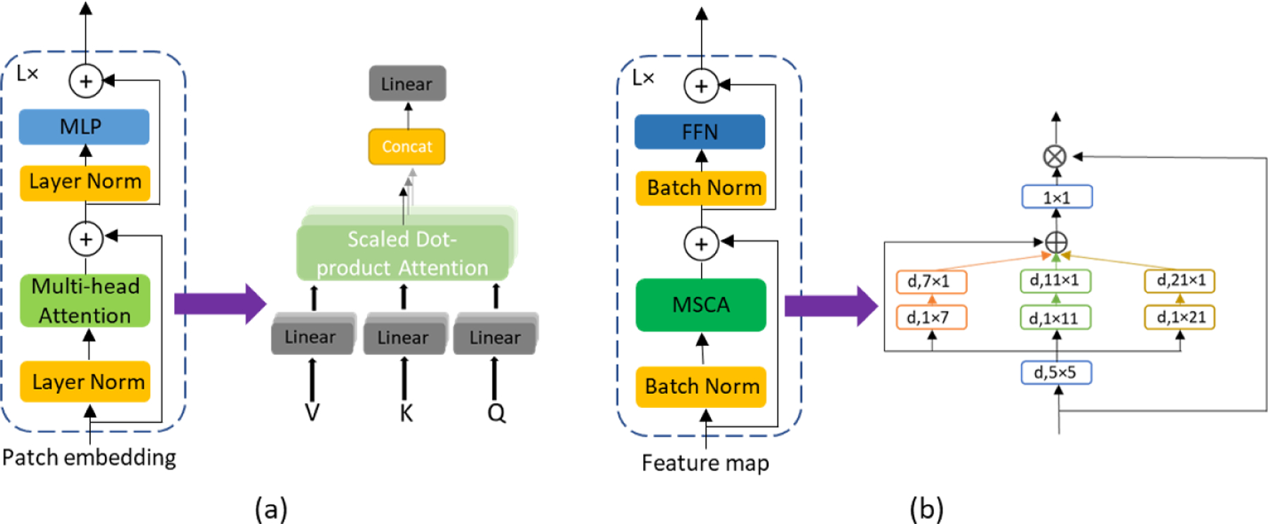
Two attention mechanisms we tested in our models. (a) Visual transformer (ViT). (b) Multi-scale convolutional attention network (MSCAN) blocks.

References

- 1.Abdollahi A, Pradhan B, Alamri A: Vnet: An end-to-end fully convolutional neural network for road extraction from high-resolution remote sensing data. IEEE Access 8, 179424–179436 (2020) [Google Scholar]
- 2.Cakir A, Dawant BM, Noble JH: Development of a ct-based patient-specific model of the electrically stimulated cochlea. In: International Conference on Medical Image Computing and Computer-Assisted Intervention. pp. 773–780. Springer; (2017) [Google Scholar]
- 3.Chen J, Lu Y, Yu Q, Luo X, Adeli E, Wang Y, Lu L, Yuille AL, Zhou Y: Transunet: Transformers make strong encoders for medical image segmentation. arXiv preprint arXiv:2102.04306 (2021)
- 4.Dosovitskiy A, Beyer L, Kolesnikov A, Weissenborn D, Zhai X, Unterthiner T, Dehghani M, Minderer M, Heigold G, Gelly S, et al. : An image is worth 16×16 words: Transformers for image recognition at scale. arXiv preprint arXiv:2010.11929 (2020)
- 5.Fan Y, Zhang D, Wang J, Noble JH, Dawant BM: Combining model-and deep-learning-based methods for the accurate and robust segmentation of the intra-cochlear anatomy in clinical head ct images. In: Medical Imaging 2020: Image Processing vol. 11313, pp. 315–322. SPIE; (2020) [Google Scholar]
- 6.Frijns JH, Briaire JJ, Grote JJ: The importance of human cochlear anatomy for the results of modiolus-hugging multichannel cochlear implants. Otology & neurotology 22(3), 340–349 (2001) [DOI] [PubMed] [Google Scholar]
- 7.Guo MH, Lu CZ, Hou Q, Liu Z, Cheng MM, Hu SM: Segnext: Rethinking convolutional attention design for semantic segmentation. arXiv preprint arXiv:2209.08575 (2022)
- 8.Hesamian MH, Jia W, He X, Kennedy P: Deep learning techniques for medical image segmentation: achievements and challenges. Journal of digital imaging 32(4), 582–596 (2019) [DOI] [PMC free article] [PubMed] [Google Scholar]
- 9.Iglesias JE, Billot B, Balbastre Y, Tabari A, Conklin J, Gonźalez RG, Alexander DC, Golland P, Edlow BL, Fischl B, et al. : Joint super-resolution and synthesis of 1 mm isotropic mp-rage volumes from clinical mri exams with scans of different orientation, resolution and contrast. Neuroimage 237, 118206 (2021) [DOI] [PMC free article] [PubMed] [Google Scholar]
- 10.Isensee F, Jaeger PF, Kohl SA, Petersen J, Maier-Hein KH: nnu-net: a self-configuring method for deep learning-based biomedical image segmentation. Nature methods 18(2), 203–211 (2021) [DOI] [PubMed] [Google Scholar]
- 11.Kalkman RK, Briaire JJ, Frijns JH: Current focussing in cochlear implants: an analysis of neural recruitment in a computational model. Hearing research 322, 89–98 (2015) [DOI] [PubMed] [Google Scholar]
- 12.Ledig C, Theis L, Husźar F, Caballero J, Cunningham A, Acosta A, Aitken A, Tejani A, Totz J, Wang Z, et al. : Photo-realistic single image super-resolution using a generative adversarial network. In: Proceedings of the IEEE conference on computer vision and pattern recognition. pp. 4681–4690 (2017) [Google Scholar]
- 13.Li Y, Sixou B, Peyrin F: A review of the deep learning methods for medical images super resolution problems. Irbm 42(2), 120–133 (2021) [Google Scholar]
- 14.Malherbe T, Hanekom T, Hanekom J: Constructing a three-dimensional electrical model of a living cochlear implant user’s cochlea. International journal for numerical methods in biomedical engineering 32(7), e02751 (2016) [DOI] [PubMed] [Google Scholar]
- 15.NIDCD: Nidcd (2019) nidcd fact sheet, hearing and balance: cochlear implants, https://www.nidcd.nih.gov/health/cochlear-implants, accessed 10 Jan 2023
- 16.Noble JH, Gifford RH, Hedley-Williams AJ, Dawant BM, Labadie RF: Clinical evaluation of an image-guided cochlear implant programming strategy. Audiology and Neurotology 19(6), 400–411 (2014) [DOI] [PMC free article] [PubMed] [Google Scholar]
- 17.Noble JH, Hedley-Williams AJ, Sunderhaus L, Dawant BM, Labadie RF, Camarata SM, Gifford RH: Initial results with image-guided cochlear implant programming in children. Otology & neurotology: official publication of the American Otological Society, American Neurotology Society [and] European Academy of Otology and Neurotology 37(2), e63 (2016) [DOI] [PMC free article] [PubMed] [Google Scholar]
- 18.Noble JH, Labadie RF, Gifford RH, Dawant BM: Image-guidance enables new methods for customizing cochlear implant stimulation strategies. IEEE Transactions on Neural Systems and Rehabilitation Engineering 21(5), 820–829 (2013) [DOI] [PMC free article] [PubMed] [Google Scholar]
- 19.Oktay O, Schlemper J, Folgoc LL, Lee M, Heinrich M, Misawa K, Mori K, McDonagh S, Hammerla NY, Kainz B, et al. : Attention u-net: Learning where to look for the pancreas. arXiv preprint arXiv:1804.03999 (2018)
- 20.Park J, Hwang D, Kim KY, Kang SK, Kim YK, Lee JS: Computed tomography super-resolution using deep convolutional neural network. Physics in Medicine & Biology 63(14), 145011 (2018) [DOI] [PubMed] [Google Scholar]
- 21.Qiu D, Cheng Y, Wang X, Zhang X: Multi-window back-projection residual networks for reconstructing covid-19 ct super-resolution images. Computer Methods and Programs in Biomedicine 200, 105934 (2021) [DOI] [PMC free article] [PubMed] [Google Scholar]
- 22.Ronneberger O, Fischer P, Brox T: U-net: Convolutional networks for biomedical image segmentation. In: International Conference on Medical image computing and computer-assisted intervention. pp. 234–241. Springer; (2015) [Google Scholar]
- 23.Wang J, Zhao Y, Noble JH, Dawant BM: Conditional generative adversarial networks for metal artifact reduction in ct images of the ear. In: International Conference on Medical Image Computing and Computer-Assisted Intervention. pp. 3–11. Springer; (2018) [Google Scholar]
- 24.Whiten DM: Electro-anatomical models of the cochlear implant Ph.D. thesis, Massachusetts Institute of Technology; (2007) [Google Scholar]
- 25.You C, Li G, Zhang Y, Zhang X, Shan H, Li M, Ju S, Zhao Z, Zhang Z, Cong W, et al. : Ct super-resolution gan constrained by the identical, residual, and cycle learning ensemble (gan-circle). IEEE transactions on medical imaging 39(1), 188–203 (2019) [DOI] [PMC free article] [PubMed] [Google Scholar]
- 26.Zhang D, Banalagay R, Wang J, Zhao Y, Noble JH, Dawant BM: Two-level training of a 3d u-net for accurate segmentation of the intra-cochlear anatomy in head cts with limited ground truth training data. In: Medical Imaging 2019: Image Processing vol. 10949, pp. 45–52. SPIE; (2019) [DOI] [PMC free article] [PubMed] [Google Scholar]