Detection of Abdominopelvic Lymph Nodes in Multi-Parametric MRI

Abstract

Reliable localization of lymph nodes (LNs) in multi-parameteric MRI (mpMRI) studies plays a major role in the assessment of lymphadenopathy and staging of metastatic disease. Radiologists routinely measure the nodal size in order to distinguish benign from malignant nodes, which require subsequent cancer staging. However, identification of lymph nodes is a cumbersome task due to their myriad appearances in mpMRI studies. Multiple sequences are acquired in mpMRI studies, including T2 fat suppressed (T2FS) and diffusion weighted imaging (DWI) sequences among others; consequently, the sizing of LNs is rendered challenging due to the variety of signal intensities in these sequences. Furthermore, radiologists can miss potentially metastatic LNs during a busy clinical day. To lighten these imaging and workflow challenges, we propose a computer-aided detection (CAD) pipeline to detect both benign and malignant LNs in the body for their subsequent measurement. We employed the recently proposed Dynamic Head (DyHead) neural network to detect LNs in mpMRI studies that were acquired using a variety of scanners and exam protocols. The T2FS and DWI series were co-registered, and a selective augmentation technique called Intra-Label LISA (ILL) was used to blend the two volumes with the interpolation factor drawn from a Beta distribution. In this way, ILL diversified the samples that the model encountered during the training phase, while the requirement for both sequences to be present at test time was nullified. Our results showed a mean average precision (mAP) of 53.5% and a sensitivity of ~78% with ILL at 4 FP/vol. This corresponded to an improvement of ≥10% in mAP and ≥12% insensitivity at 4FP (p < 0.05) respectively over current LN detection approaches evaluated on the same dataset. We also established the out-of-distribution robustness of the DyHead model by training it on data acquired by a Siemens Aera scanner and testing it on data from the Siemens Verio, Siemens Biograph mMR, and Philips Achieva scanners. Our pilot work represents an important first step towards automated detection, segmentation, and classification of lymph nodes in mpMRI.

1. Introduction

Lymph nodes (LNs) are small structures scattered throughout the body and are a part of the lymphatic system. Lymphocytes (immune cells) in the LNs travel through the nodal network in search of certain target proteins that need to be filtered and removed from the body. An abnormal proliferation of lymphocytes in some patients can result in swollen lymph nodes or lymphadenopathy (Ruby and Shivaraj (2022)); this could be due to many reasons, such as infections, autoimmune disease, and malignancy. In these patients, enlarged and metastatic nodes need to be distinguished from benign nodes (Taupitz (2007)). It is especially crucial to identify enlarged LNs if they are found at sites that do not correspond to the first site of lymphatic spread as this signals distant metastasis (Taupitz (2007)). Multi-parametric MRI (mpMRI) is a common imaging method used to detect abnormal LNs. In mpMRI, various sequences are obtained, such as T2-weighted series, T2 fat suppressed (T2FS) series, Diffusion Weighted Imaging (DWI), and derived Apparent Diffusion Coefficient (ADC) maps. The American Joint Committee on Cancer (AJCC) provide guidelines (Amin et al. (2017)) on the measurement of nodal size, location, and number of LNs to be evaluated for patient treatment. With the help of these guidelines, radiologists routinely measure the size of LNs with the long- and short-axis diameters (LAD and SAD) to determine the metastatic nature of lymph nodes. Nodes with a SAD ≥ 1cm on T2FS sequences are considered suspicious for metastasis (Taupitz (2007)), and a correlation with a different series (e.g., DWI and ADC) is typically sought for malignancy confirmation.

Clinically, it is important to identify lymph nodes with a SAD ≥ 1cm and bring them to the attention of the radiologist reading the study, such that they measured and assessed appropriately. However, precise measurement of LNs is challenging due to the diverse appearances and shapes of LNs in mpMRI. Additional confounding factors that complicate the assessment are the variety of imaging scanners built by different manufacturers, their myriad uses at different imaging institutions/centers, exam protocols utilized by the imaging technologist, institutional guidelines for LN assessment, and observer measurement variability among others. Furthermore, sizing of various structures (e.g., lesions, nodules, LNs) at various locations in the body is a routine and repetitive task within a radiologist’s daily workflow. During a busy clinical day, it is possible that some suspicious structures may be missed. To relieve this time-consuming and cumbersome nature of repetitive measurements, a artificial intelligence (AI) algorithm that can account for all these factors is clinically necessary.

In the past, several algorithms have been proposed for LN identification (Zhao et al. (2020); Lu et al. (2018); Debats et al. (2019); Mathai et al. (2021, 2022a); Wang et al. (2022); Mathai et al. (2022b)). Certain approaches focus on detecting LNs in specific regions of body, such as the pelvis (Debats et al. (2019); Lu et al. (2018)) and rectum (Zhao et al. (2020)). Debats et al. (2019) extracted patches from the slices of MR lymphography studies of the pelvis and fed them to a convolutional neural network to classify metastatic and normal lymph node tissue. Other research works (Mathai et al. (2021, 2022a); Wang et al. (2022); Mathai et al. (2022b)) for the detection of both benign and malignant lymph nodes also exist; T2FS MRI volumes were used in these approaches to train a variety of neural networks, such as Mask RCNN (Wang et al. (2022)), Detection Transformer (Mathai et al. (2022a)), and ensemble-based approaches (Mathai et al. (2021, 2022a,b)). However, the utility of multi-parametric MRI studies has not been widely studied and there are only a few approaches for this task (Zhao et al. (2020); Lu et al. (2018)). Lu et al. (2018) trained a Faster RCNN model on LNs annotated in slices of both T2FS and DWI series (sequences were not registered to each other) from mpMRI studies, and classified the status of LNs in a test set as benign or malignant. Zhao et al. (2020) used a Mask RCNN model to detect and segment LNs in the rectal region of pelvic mpMRI studies. Both T2FS and DWI series were used and 3-channel input images were constructed for training the Mask RCNN model. The authors investigated various combinations of T2FS and DWI slices (e.g., 2 T2FS slices + 1 DWI slice) as input. Since DWI or ADC may not always be acquired, relying on the presence of a DWI sequence may not be ideal.

In this work, we present an automated pipeline for lymph node detection in mpMRI studies. Our pipeline uses the T2FS and DWI sequences from an mpMRI study, and harnesses a Dynamic Head (DyHead) network (Dai et al. (2021)) to detect LNs (metastatic and non-metastatic) for subsequent measurement. The T2FS and DWI series were co-registered, and then linearly interpolated together to create a blended volume using a selective data augmentation technique called Intra-Label LISA (ILL) (Yao et al. (2022)). The blended volume contained traits of both series, such as fat suppression and diffusion restriction. The mpMRI studies were acquired at our institution using various MR scanners (Siemens and Philips) and a variety of exam protocols, and model training was done with the clinical annotations of LAD and SAD measurements by radiologists directly. At test time, data presented to the model could come from either the T2FS series alone, or from the blending of any available T2FS and DWI series that were co-registered. Contrary to prior work (Zhao et al. (2020); Wang et al. (2022)), we also used full-size input data for training and testing. The main contributions of this work include the use of ILL to diversify the input data samples the model encountered during training, and the integration of the complete IoU loss Zheng et al. (2022) in the DyHead framework. With their inclusion, our model did not rely on the presence of both T2FS and DWI series in the mpMRI study.

2. Materials and Methods

2.1. Data

The Picture Archiving and Communication System (PACS) at the NIH Clinical Center was queried for patients who had undergone MRI imaging between January 2015 and September 2019. Initially, a total of 383 patients (224 males and 159 females with ages between 6 and 85 years) and 500 mpMRI studies were identified. The radiology report associated with a study was obtained, and a natural language processing algorithm developed by Peng et al. (2020) extracted the presence of metastatic and/or non-metastatic LNs, extent, and size measurements. The results from the NLP algorithm were validated by a radiologist for inclusion into the data cohort. Each study contained various series such as T2 weighted (T2WI) series, T2 fat suppressed (T2FS) series, diffusion weighted imaging (DWI) and apparent diffusion coefficient (ADC) maps. However, the studies did not always contain DWI and ADC series. These studies were acquired using a variety of MRI scanners (Siemens, Philips) and exam protocols. At our institution, radiologists sized the LNs by scrolling back and forth across the slices in the T2FS series, matched the appearance of suspicious nodes in the DWI series, and measured the largest LN extent present on a single 2D slice in the T2FS series according to the routine clinical protocol for measuring LNs. LNs were measured with either the long axis diameter (LAD) or short axis diameter (SAD), or both simultaneously. As it is cumbersome for radiologists to measure the full 3D extent of suspicious LNs during a busy clinical day, the primary measurement of LAD and SAD was prospectively made only on a single 2D slice. If only a single measurement (LAD or SAD) was done, a radiologist conducted a quality check to ensure that both LAD and SAD measurements were available.

Next, the studies containing both T2FS and DWI series were identified. In these studies, there were often multiple DWI sequences (minimum 1, maximum 3) acquired with low (0 – 200 s/mm²), intermediate (400 – 800 s/mm²), and high (800 – 1400 s/mm²) b-values. Higher b-values permit the sensing of slow moving water molecules that diffuse shorter distances within tissue. In contrast to normal tissue, the diffusion of water molecules in abnormal LNs is restricted by cell membranes, and this corresponded to a higher signal intensity in areas with diffusion restriction when visualized with DWI series. For our work, we exploited all the available DWI sequences with different b-values. This process yielded 232 patients (145 males and 87 females with ages between 6 and 80 years) with 271 mpMRI studies wherein both T2FS and DWI series were available. As the radiologists measured LNs in the T2FS series only, the DWI series were registered to T2FS to transfer the LN annotations. A rigid registration method available in the open-source Insight ToolKit (ITK) McCormick et al. (2014) was used to generate the co-registered volumes with the same origin, resolution, and spacing. Then, the studies were randomly divided on a patient-level into ~68% train (161 patients, 183 studies, 440 slices), ~8% validation (15 patients, 22 studies, 53 slices), and ~24% test (56 patients, 66 studies, 851 slices) splits. In order to provide quantitative results for this work, the 3D extent of all LNs in the test set were fully labeled with bounding boxes by the same radiologist who conducted the aforementioned quality check. AJCC Tumor, Node, and Metastasis (TNM) guidelines (Amin et al. (2017)) was used by the radiologist for the full 3D extent annotation. However, the train and validation splits consisted of only the prospective 2D measurements made by the radiologist that originally read the study. N4 bias normalization Tustison et al. (2010) was subsequently performed on the co-registered sequences, followed by normalization to [1%, 99%] of the voxel intensity range Kociołek et al. (2020), and histogram equalization Chen et al. (2015) to boost the contrast between bright and dark structures in the volumes. The resulting data had various dimensions in the range of (256 ~ 640) × (192 ~ 640) × (18 ~ 60) voxels.

2.2. Selective Augmentation

For the pipelines in previous approaches (Zhao et al. (2020); Lu et al. (2018)) to work, both the T2FS and DWI series needed to be present. However, the presence of both sequences cannot always be guaranteed as a complete MRI workup is not always deemed medically necessary by the referring physician or the radiologist, and thus certain sequences may not be acquired. Therefore, it is necessary to take full advantage of the available sequences in an mpMRI study for training a LN detector. In this work, we use a recently proposed method by Yao et al. (2022) to learn invariant representations via selective augmentation (LISA). LISA interpolated the training data samples that have the same label, but were sampled from different domains (T2FS and DWI). Since the T2FS and DWI sequences are co-registered to each other, the label (bounding boxes) from the T2FS sequence can be transferred to DWI. Specifically, we use Intra-Label LISA (ILL) to selectively augment our training data; we blend the T2FS and DWI sequences together so that traits of both series are visible in the same volume. The blending is rooted in the MixUp (Zhang et al. (2018)) and CutMix (Yun et al. (2019)) techniques, which linearly interpolate training data samples and remove any correlations (Cramér (2016)) between the domain and labels. Through this simple trick, the LN detector can learn invariant predictors for LNs. Formally, assume that two data samples (x_i, y_i, d_i) and (x_j, y_j, d_j) are drawn from two distinct domains d_i and d_j. Two samples can be linearly interpolated according to:

$$x_m=\lambda x_i+(1-\lambda )x_j\hspace{1em}\text{and}\hspace{1em}{y}_m=\lambda y_i+(1-\lambda )y_j$$ (1)

$$\widehat{\theta }:=\underset{\theta \in \Theta }{\text{argmin}}{\mathbb{E}}_{\left\{\left(x_i,y_i,d_i\right),\left(x_j,y_j,d_j\right)~\widehat{P}\right\}}\left[l\left(f_{\theta }\left(x_m\right),y_m\right)\right]$$ (2)

where λ ∈ [0, 1] is the interpolation ratio sampled from a Beta distribution Beta(α, β), and dictates the strength of blending for selective augmentation. Since the label (bounding box) is the same y_i = y_j for the co-registered T2FS and DWI series, interpolation of the data samples results in volumes where characteristics of both domains are partially present and any spurious correlations that exist between the domains and labels are removed. This gives rise to an empirical risk minimization setting as in Eqn. 2 where given a training distribution P_tr, a loss function l is used to train a model f_θ to optimize its parameters θ ∈ Θ. As the parameters of the beta distribution govern the blending ratio λ, it permitted the use of either the T2FS sequence alone or a combination of T2FS and DWI series. If a study did not contain the DWI series, then ILL was not applied. The need for both series to be present in an mpMRI study was thereby circumvented, and it enabled the model to encounter diverse examples during training to enhance robustness against noise at the test time. Experiments conducted in Sec. 3 attest to the advantage of using our simple selective augmentation approach for LN detection. Examples images using ILL-based blending are shown in Fig. 2.

Fig. 2:

Our proposed Dynamic Head (DyHead) model detected a large lymph node (LN) of size 1.3cm straddling the kidney. Results are shown for 5 consecutive slices. The mpMRI study used here contained a T2 Fat Suppressed (T2FS) series and a Diffusion Weighted Imaging (DWI) series. In each row, the T2FS slice is on the left, a DWI slice is in the middle, and a blend of T2FS and DWI slices is on the right. The blended slice was generated by first co-registering the T2FS and DWI series, and then blending them together using Intra-Label LISA (ILL). Our proposed DyHead model was trained on these blended volumes to predict 2D LN candidates in each slice. Next, our 3D clustering technique combined the 2D predictions into 3D, and the resulting boxes were overlaid for visualization. Green boxes: ground truth, yellow: true positives, red: false positives. The text below each detected box, e.g. “52 | 49”, describes the highest confidence score across all elements of the 3D prediction followed by the confidence score of the candidate box detected in the current slice. Figure best viewed in the PDF in color.

2.3. Model

The standard design of an object detector consists of a backbone network to extract features, followed by a network head tasked with the classification and localization of objects seen in an image. For identifying specific regions of interest (ROIs) in medical images, there are many considerations to take into account while designing a detection head. First, the scale of structures is important as they can be large (e.g. liver) or small (e.g., lymph nodes, lesions). Second, there can be multiple ROIs present close to each other, and distinguishing them individually is critical for many tasks (e.g., organ/lesion volume measurements). Finally, ROIs can be represented in many ways (e.g., bounding boxes, centers, segmentation masks); the ROI representation plays a crucial role in the set of tasks the network is assigned to solve.

In this work, we employed the recently proposed detection network called Dynamic Head or DyHead (Dai et al. (2021)). DyHead combined the scale-, spatial-, and task-aware attention mechanisms into the detection head of the adaptive training sample selection (ATSS) framework (Zhang et al. (2020)). The input to the ATSS + DyHead model after the co-registration process and blending with ILL was a 2.5D image that contained three consecutive slices from the blended volume with the slice in the middle containing the annotated LN. The feature maps ${\left\{F_i\right\}}_i^L$ from each of the L levels of the backbone network (Lin et al. (2017)) were resized through up-/down-sampling to the shape of the median level features. This resulted in a 4D feature tensor of dimensions L × H × W × C, where H and W are the height and width of a feature map respectively, and C is the number of output channels for the median FPN level. The 4D tensor was then reshaped into a 3D tensor of dimensions L × S × C, where S = H × W, such that the different attention mechanisms could be applied across the level × space × channels dimensions respectively.

Feature maps at different levels of the backbone inherently capture the variety of sizes and scales of the LNs in the mpMRI studies used in this work. Therefore, the scale-aware attention module was applied on the level dimension and it dynamically changed the relative importance placed on the various levels of the backbone network. Moreover, LNs can straddle major anatomical structures (e.g., liver, bowel, blood vessels) and appear in close proximity to each other. The spatial-aware attention module applied to the space dimension enabled the network to discriminate LNs in different spatial locations. Feature maps at different levels could also be bundled together for effective localization. Finally, specific sub-tasks, such as bounding box and center-point regression, were critical to achieve the main task of detecting the 3D extent of LNs. The task-aware attention module implemented on the channels dimension emphasized the significance of certain channels more for a particular task. As shown in Fig. 1, the different feature maps extracted from the different attention mechanisms showcased the scale-awareness to the relative size of various LNs, spatial-awareness to the location of each LN, and task-awareness with respect to bounding box and center-point regression.

Fig. 1:

Flowchart of the proposed computed-aided detection (CAD) pipeline. First, T2FS and DWI series in an mpMRI study were co-registered and then blended together using Intra-Label LISA (ILL). Next, three consecutive slices from the resulting volume were collated to form a 3-channel image. The images are then fed to the Dynamic Head (DyHead) detector based on the ATSS framework, which predicted bounding boxes for potential lymph nodes (LNs) in each slice of the volume. Green boxes: ground truth, yellow: true positives, red: false positives. Feature maps that are used by the network for prediction are shown. Compared to the feature maps generated by the backbone (Swin Transformer) of the DyHead network, the scale-aware attention module distinguishes the correct scales of two neighboring LNs close to liver, the spatial-aware attention module correctly identifies the distinct spatial locations of the LNs, and the task-aware attention module focuses the learning on specific representations of the LNs (e.g., bounding boxes, centers etc.). The 2D LN candidates were then merged into 3D based on their confidence scores as well as their IoU overlaps with boxes in adjacent slices. Figure best viewed in the PDF in color.

To generate informative feature maps for DyHead, we used the general-purpose Swin Transformer backbone Liu et al. (2021) in the ATSS + DyHead framework instead of the original ResNet-50 backbone. The rationale behind this was due to the hierarchical feature maps computed by the Swin transformer; they have the same dimensions as those obtained from standard backbones, such as ResNet (He et al. (2016)) and FPN (Lin et al. (2017)). These hierarchical feature maps were estimated by first splitting the input image into small-sized image patches in shallower layers and merging neighboring patches in deeper layers. A fixed number of image patches were then taken to constitute a window, within which self-attention was computed locally. Shifted window partitioning also introduced connections across neighboring windows that increased the representation modeling power while also maintaining linear computation complexity. For more details on the implementation, we refer the reader to Liu et al. (2021). Through experiments described in Sec. 3, we show that the model was able to achieve higher precision and sensitivities at different FP with the Swin transformer backbone.

Additionally in this work, we integrated the complete-IoU (CIoU) loss proposed by Zheng et al. (2022) in the ATSS framework instead of the generalized IoU (GIoU) loss Rezatofighi et al. (2019). The GIoU loss focused primarily on the overlap area between two boxes and tried to maximize the overlap value during the training process leading to a longer convergence time. On the other hand, CIoU loss considered geometric factors related to the box regression, such as overlap area, normalized center-point distance, and aspect ratio. This is of particular importance as LNs in mpMRI have myriad shapes and appearances, making the task of distinguishing them and regressing their box coordinates challenging. After the model had been trained, Weighted Boxes Fusion (WBF) Solovyev et al. (2021) was used to combine the various predictions from the best epochs of multiple runs of the same model. LN detection results by the DyHead model on 3 consecutive slices from a volume are shown in Figs. 2 and 3.

Fig. 3:

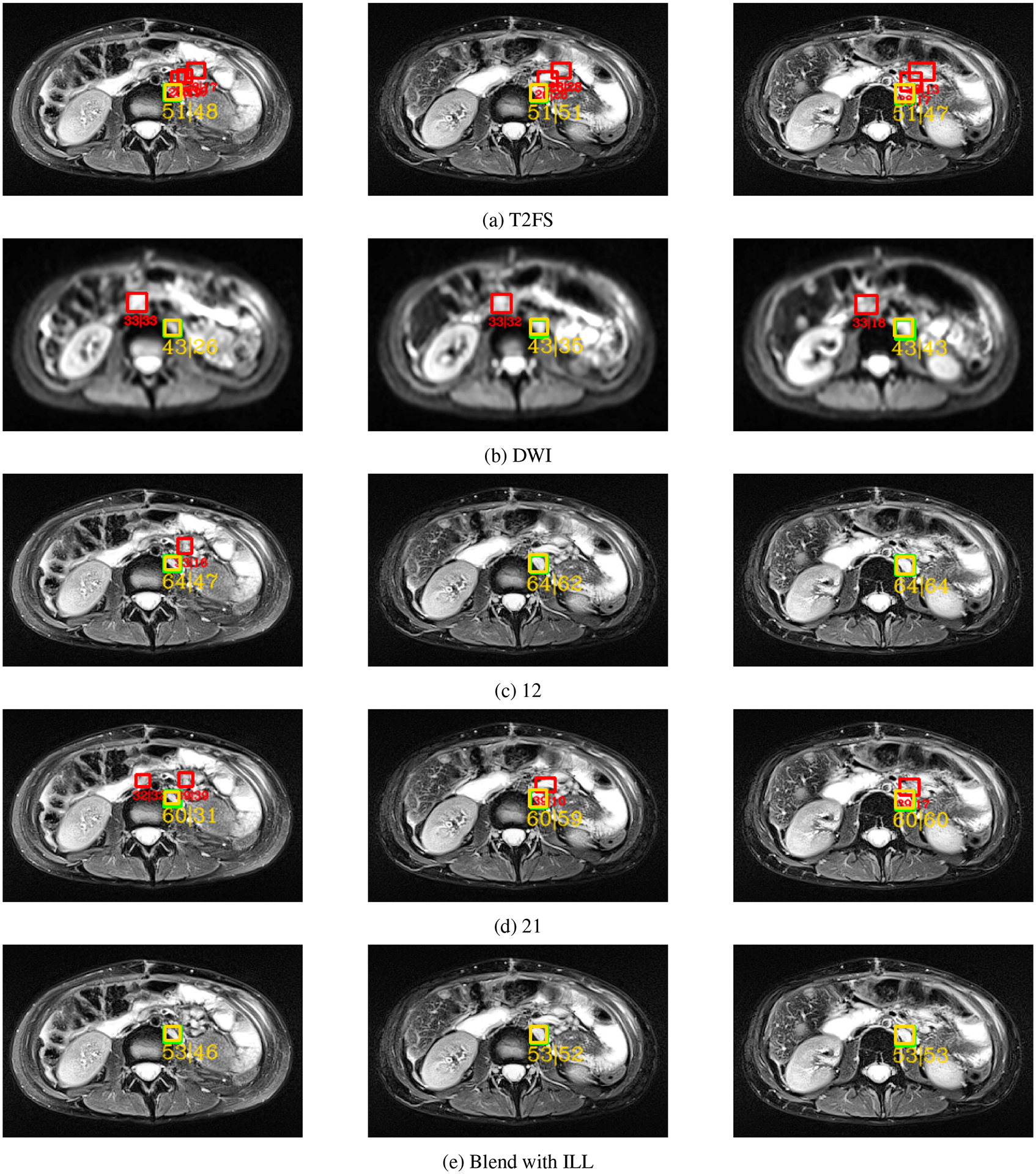
A normal sized LN (8mm) straddling the kidney was detected on 3 consecutive slices. Each row shows the predictions obtained from one of five different DyHead models trained with different data combinations. In row (a), the DyHead model was trained with only T2FS series, whilst in row (b), it was trained on only DWI series. In row (c), a combination of 1 slice of T2FS and 2 slices of DWI series respectively was used. In row (d), a combination of 2 slices of T2FS and 1 slice of DWI series respectively was used. Finally in row (e), the DyHead model was trained with slices extracted from the blended volume generated with selective data augmentation. Green boxes: ground truth, yellow: true positives, red: false positives. The text below each detected box, e.g. “51 | 48”, describes the highest confidence score across all elements of the 3D prediction followed by the confidence score of the candidate box detected in the current slice. Notice that there are fewer FP predictions in row (e) with the proposed selective data augmentation in contrast to the other data combinations. Figure best viewed in the PDF with color.

2.4. 3D Prediction Generation

Our DyHead model predicted LN candidates in every slice of the blended volume, and these 2D proposals were later post-processed into 3D predictions. Each 2D prediction contains the coordinates of the enclosing bounding box of the potential LN along with a confidence score. Next, we follow the Kalman filter-based bounding box tracking approach as proposed in Yang et al. (2019) and Cai et al. (2021). First, we filter the 2D predictions based on their confidence score and keep a prediction if it has a confidence ≥ 10%. Our rationale was to remove only the boxes with low scores while preserving those that represent a true LN detection despite their scale in the current slice. Next, as seen in Fig. 1, we created the 3D clusters by stacking the 2D predictions together from pairs of adjacent slices when their IoU overlap score was ≥ 25%. Contrary to Yang et al. (2019), we chose this threshold value as it accounted for the large variations in voxel sizes (especially along the z-axis) for volumes acquired by different MRI scanners. Finally, we filtered the clusters based on the maximum confidence score available in that cluster and removed those that did not cross a confidence threshold of 30%. We chose this value in order to keep the number of 3D predictions manageable.

3. Experiments

3.1. Comparison with state-of-the-art approaches

Our main experiment E_SA used co-registered T2FS and DWI sequences, blended them through ILL, and detected LN in them. 2.5D images were extracted from the blended volume with each image containing three consecutive slices from the volume with the annotated LNs present in the slice in the middle. This approach mimicked prior work in Debats et al. (2019), where the authors detailed that the in-plane slice provided the most salient information necessary for LN detection. We compared our method against other works: 1) Existing state-of-the-art object detectors, such as Faster RCNN by Ren et al. (2015), VarifocalNet or VFNet by Zhang et al. (2021) and DDOD by Chen et al. (2021). 2) We contrasted our results against the re-implementation in Zhao et al. (2020), in which the authors cropped the 2.5D images to 256 × 256 pixels encompassing the LNs in the rectal region. 3) We compared our results against those published by Wang et al. (2022), wherein a universal LN detector was trained with only T2FS volumes, from which 2.5D images were constructed for training. 4) Finally, we followed the approaches proposed in prior works by Mathai et al. (2022a, 2021, 2022a,b, 2023), and created an ensemble from the object detectors for LN detection.

For consistent comparison across all works, we did not crop our slices and used the full-sized images as training inputs. Both Zhao et al. (2020) and Wang et al. (2022) used a Mask RCNN model for detection and segmentation of LNs. However, we did not possess segmentation labels in this work. In order to conduct a fair comparison, we used a close relative in the Faster RCNN model and re-implemented their works after a grid search to find the best hyper-parameters. Additionally, Zhao et al. (2020) conducted four experiments with different combinations of T2FS and DWI slices including: 1) 3-slices of only T2FS (E_T), 2) 3-slices of only DWI (E_D), 3) 1-slice of T2FS and 2-slices of DWI (E₁₂), and 4) 2-slices of T2FS and 1-slice of DWI (E₂₁). We also performed the same experiments to achieve fair comparisons across the state-of-the-art object detectors.

3.2. Comparison of blending parameters for selective augmentation

One of the main contributions in this work is the selective augmentation of the data through blending of co-registered T2FS and DWI series. Since the Beta distribution governed the blending of the two sequences, we evaluated the effect of the choice of its parameters. The DyHead network was trained with an interpolation ratio λ selected from the beta distribution Beta(α, β) with α = 2 and β = 2. Other parametric choices that were tested included Beta(1, 1), such that λ was drawn from a uniform distribution as examined by Yun et al. (2019), and Beta(4, 4). We also evaluated the effect of drawing λ from a Beta(60, 10) distribution that heavily favored the T2FS series.

3.3. Comparison of network backbone and IoU-based losses

Two other contributions that were made in this work were the utilization of the Swin Transformer backbone in the the ATSS framework instead of the ResNet-50 backbone, and the complete IoU (CIoU) loss instead of the traditional IoU losses (e.g., IoU, GIoU) respectively. Our aim was the test the information provided by the hierarchical feature maps generated by the Swin Transformer backbone. We also wanted to assess the utility of the geometric factors (aspect ratio, overlap area, and normalized center-point distance) considered by the CIoU loss formulation in contrast to the traditional IoU-based losses that mainly focused on maximizing the overlap area between two boxes.

3.4. Out-of-distribution comparison

We wanted to evaluate the robustness of the DyHead model to out-of-distribution (OOD) data under the condition of domain shift. However, the underlying distributions of the Siemens (Aera, Verio, BioGraph mMR) and Philips (Achieva) scanners were unknown in this work. Diving deeper into our dataset (232 patients, 271 studies), we found that the data acquired by the Siemens Aera scanner comprised a major part of our dataset (204 patients, 236 studies). There were limited data quantities from other scanners: Siemens Verio (14 patients, 15 studies), Siemens Biograph mMR (11 patients, 11 studies), and Philips Achieva (3 patients, 9 studies). Therefore, we created an experiment where only the data from the Siemens Aera scanner was used to train the DyHead model, and it was tested on data from the remaining MRI scanners.

3.5. Implementation

In our work, 2.5D (3-channel) images were used to train the detectors, which were implemented with the mmDetection framework (Chen and et al. (2019)). Apart from the use of ILL-based blending, standard data augmentation was performed, such as random flips, crops, shifts and rotations in the range of [0, 32] pixels and [0, 10] degrees respectively, random contrast and gamma adjustments. ResNet-50 was the backbone (pre-trained with MS COCO weights) used for Faster RCNN, VFNet, and DDOD. A grid search was run across the different hyper-parameter settings to obtain the optimal values for the different models tested in this work. The summary of these hyper-parameters are shown in Table. 1. We ran a 5-fold cross-validation scheme where each model was executed 5 times with different training data subsets. The test set was held-out and kept the same across the different folds. We saved the top-5 checkpoints with the lowest validation loss from each run, and used the checkpoint from each run with the lowest loss (total of 5 model checkpoints) for testing. Results presented in Table 2 were an average of 5-fold cross-validation. All experiments were run on a NVIDIA DGX workstation running Ubuntu 18.04LTS with 4 Tesla V100 GPUs. Evaluation was performed at an IoU threshold of 25% to be consistent with prior work as in Zhao et al. (2020); Wang et al. (2022); Mathai et al. (2022b).

Table 1:

Hyper-parameter settings and runtime information for the various LN detection models.

Setting	Faster RCNN	VFNet	DDOD	DyHead
Backbone	ResNet-50	ResNet-50	ResNet-50	Swin
Batch size	8	4	8	2
Epochs	12	12	12	12
Learning rate	1e−3	1e−3	1e−4	5e−5
Activation function	ReLU	ReLU	ReLU	ReLU
Optimizer	SGD	SGD	SGD	AdamW
# parameters (million)	41.7 M	75.2 M	86.1 M	158.7 M
GFLOPs	19.3	106.1	134.8	327.6
Inference Time (sec/vol)	3.1	4.7	5.3	6.2

Table 2:

Performance comparison of different methods on the 3D test dataset. “Exp” stands for the experimental abbreviation and “Mode” describes the {T2FS, DWI} data combination mode. “SA” and “NSA” indicate selective and no selective augmentation respectively, while “ILL” stands for Intra-Label LISA. “S” describes Sensitivity @[0.5, 1, 2, 4] FP. Bold values indicate best results.

#	Method	Exp	Mode	mAP	S@0.5	S@1	S@2	S@4
1	Faster RCNN Ren et al. (2015)	E SA	ILL	48.7	32.7	45.5	57.4	68.3
2	VFNet Zhang et al. (2021)	E SA	ILL	51.1	31.7	46.5	60.4	74.8
3	DDOD Chen et al. (2021)	E SA	ILL	49.9	26.7	42.1	59.4	71.3
4	Wang 2022 (2D) Wang et al. (2022)	E t	T2FS only	40.3	30.1	36.0	46.3	57.3
5	Zhao et al. (2020)	E21	NSA	43.3	24.3	39.6	55.9	65.4
6	Ensemble (1–4) Mathai et al. (2022b)	E SA	ILL	50.3	33.2	46.5	55.9	73.3
7	DyHead (Ours)	E SA	ILL	53.5	33.6	47.5	62.9	77.7
8	DyHead (Ours on T2FS)	E SA	ILL	53	32.6	45.9	57.4	75.8

3.6. Metrics

We utilized prospective 2D measurements of the LAD and SAD made by radiologists at our institution. This is because the radiologists only annotated the extent of a suspicious LN in one slice of the T2FS series, and did not annotate the 3D extent due to the time constraints of a busy clinical day. Prior approaches (Zhao et al. (2020); Wang et al. (2022)) also operated on these 2D measurements, but they reported their results based on these 2D measurements. This posed an issue as it did not reflect the true performance of a LN detector. Any correct predictions made by the network on any unmeasured LN in the same slice or the adjacent slice(s) would be counted as false positives when they should actually be counted as true positive predictions instead. Furthermore, we believe that automated methods should process the entire volume and report results on a volumetric level as opposed to a slice-based level. These results will reflect the true nature of the lymph node detection performance, and to that end, we adopt the pseudo-3D (P3D) IoU metric proposed by Cai et al. (2021). Specifically, we denote the slice containing the 2D annotation by the radiologist as z and the corresponding bounding box that resulted from that measurement as $\left(x_1,x_2,y_1,y_2,z,z\right)$. We represent a 3D prediction by $\left(x_1^{*},x_2^{*},y_1^{*},y_2^{*},z_1^{*},z_2^{*}\right)$. The P3D IoU metric assigns a 3D prediction as a true positive if and only if $z_1^{*}\le z\le z_2^{*}$ and the $IoU\left[\left(x_1,x_2,y_1,y_2\right),\left(x_1^{*},x_2^{*},y_1^{*},y_2^{*}\right)\right]\ge 50\text{\%}$. Otherwise, the 3D prediction is a false positive. For more information regarding the P3D IoU metric, we refer the reader to Cai et al. (2021). We also quantified the performance with the mean average precision (mAP).

3.7. Statistical analysis

Statistical analysis of the results was performed using the bootstrapping method proposed by Samuelson et al. (2007); Platel et al. (2014); Samulski and Karssemeijer (2011). We used the area under the Free-response Receiver Operating Characteristic (FROC) curve (A_z) as the performance measure. Patient studies were sampled with replacement from the test dataset; each bootstrapped sample consisted of 56 studies (only 1 study per patient) randomly selected from the test dataset. If a patient had > 1 study, then 1 study was randomly chosen. The two LN detection methods being compared were run on the sample to generate two FROC curves, and the difference between the area under the curves ▽A_z was estimated. The bootstrapping method was run 1000 times and generated 1000 values for ▽A_z. The p-values were defined as the fraction of values that were negative or zero. Any difference in performance was considered significant if p < 0.05.

4. Results

4.1. Results from state-of-the-art comparisons

Based on prior work by Zhao et al. (2020); Wang et al. (2022); Mathai et al. (2022b), a clinically acceptable result for LN detection meant a sensitivity of 65% at 4–6 FP per volume. Fig. 5 displays the FROC curves for the different state-of-the-art object detectors tested in this work; we show the effects of selective data augmentation with ILL alongside the various data combinations that were proposed by Zhao et al. (2020). Table 2 summarizes the results for the various detectors. DyHead trained with selective data augmentation (E_SA) achieved the best LN detection performance of 53.5% mAP and 77.7% at 4 FP/volume over the other detectors (p < 0.05). Fig. 5 shows that the experiment E_T that used the T2FS series alone provided sensitivities of ~60% – 70% at 4 FP/vol across the networks, while the experiment E_D that used the DWI series alone yielded low LN detection sensitivities of 55% – 65% at 4FP/vol across the different detectors (p < 0.05). These results are not surprising as the tissue structures in DWI series appear diffused with poor spatial resolution in contrast to the T2FS series. Furthermore, Zhao et al. (2020) found in their experiment E₁₂ that the data combination of 1 T2FS slice and 2 DWI slices worked best. Contrary to their findings, we observed that the experiment E₂₁ with the data combination of 2 T2FS slices and 1 DWI slice generally performed better than E₁₂, E_T and E_D (p < 0.05). This may be due to the contextual information available to the network from the provision of full-sized input images, instead of the cropped images around the rectum as implemented by Zhao et al. (2020). Furthermore, we passed only T2FS data (no blending) as input to the DyHead model (trained with ILL-based blending), and noticed that the results (Table 2, rows 7 and 8) were similar. These results support our idea that the model could be trained with studies containing both T2FS and DWI series, but it did not require the DWI series to be present at test time.

Fig. 5:

FROC curves for the different state-of-the-art object detectors, such as Faster RCNN, VFNet, DDOD and DyHead. The purple curves depict the sensitivity at different false positive rates for each network when they were trained with the blended volumes yielded by intra-label LISA (ILL). We also show the comparative results of the networks trained with different data combinations (see Sec. 3.1). Note that training with blended volumes consistently outperformed the other experiments (p < 0.05).

As Wang et al. (2022) also attempted to universally detect LN in T2FS MRI, we compared our results against their work. We observed an increase in mAP of ≥10% (53.5% vs. 40.3%) and a sensitivity improvement of ≥19% (77.7% vs. 57.3%) at 4 FP/volume with p < 0.05. Although these results were obtained after the reimplementation of their work with a Faster-RCNN model, comparison with their published values was not possible as they provided results in terms of 5 FP/image instead of 4 FP/volume. Finally, Mathai et al. (2022b) also detected LN in T2FS MRI using an ensemble of neural networks and we also compared our results against their work. We noticed an improvement in mAP of ≥3% (53.5% vs. 50.3%) and a sensitivity increase of ≥4% (77.7% vs. 73.3%) at 4 FP/volume (p < 0.05). Fig. 4 visually illustrates the LN detection results by the various LN detectors compared in this work on 3 consecutive T2FS slices in an mpMRI study. Figs. 2 and 3 show the LN detection results of the DyHead model on 3 consecutive slices in an mpMRI study respectively.

Fig. 4:

A small LN (6mm) in the pelvis was detected on 3 consecutive slices. Each row corresponds to the predictions obtained from a different detector: (a) Faster RCNN, (b) VFNet, (c) DDOD, and (d) DyHead. Green boxes: ground truth, yellow: true positives, red: false positives. The text below each detected box, e.g. “78 | 72”, describes the highest confidence score across all elements of the 3D prediction followed by the confidence score of the candidate box detected in the current slice. Notice that there are fewer FP predictions detected by DyHead in row (e) compared to the detectors. Figure best viewed in the PDF in color.

4.2. Results of ablation studies

First, we focused our attention on the ATSS + DyHead model and present the evaluation results for the choice of Beta distribution parameters used in ILL in Fig. 6(a). We noted an improvement in mAP of ~2% and sensitivity of ~4.5% at 4 FP/vol when the DyHead model was trained with the Beta distribution Beta(2, 2) over other choices. Next, we compared the effect of using the Swin transformer backbone network in place of the ResNet-50 backbone network. As shown in Fig. 6(b), we saw a rise in mAP of ~8% (53.5% vs. 44.6%) and sensitivity of ~10% at 4 FP/vol (77.7% vs. 67.3%) through the use of the Swin transformer backbone, thereby attesting to the utility of the generated hierarchical feature maps for LN detection. Similarly, we compared the integration of the complete-IoU (CIoU) loss in the DyHead network against the traditional IoU-based losses, e.g., GIoU and IoU. As seen in Fig. 6(b), we noticed an increase of ~5% in mAP and ≥4% in sensitivity at 4 FP/vol with the use of CIoU loss.

Fig. 6:

(a) FROC curves for the ablation studies of the Beta distribution Beta(α, β) parameter choice used in the ILL-based volumetric blending technique employed in this work. (b) FROC curves for the ablation studies of the complete IoU (CIoU) loss function used in this work in contrast to the traditional IoU-based losses, as well as the ablation experiment for the ResNet-50 backbone used in the ATSS framework. Note that the purple curves indicating the modifications made to the ATSS + Dyhead framework used in this work consistently outperformed the other methods at a sensitivity measure of 4 FP/volume (p < 0.05).

4.3. Results of out-of-distribution study

Table 3 summarizes the experimental results that evaluated the robustness to out-of-distribution data from other MRI scanner types. Fig. 7 showcases the detected LNs in images extracted from mpMRI studies acquired by different scanners. Our DyHead model was able to achieve comparable performance in terms of mAP and sensitivity across the data subsets from different scanners. The model had the highest mAP of ~65% for data from the Philips Achieva scanner while the highest sensitivity of ~80% at 4 FP/vol was achieved for the Siemens BioGraph mMR scanner. Overall, the results attest to the robustness of our DyHead model in detecting LNs by handling data arising from different MRI scanners.

Table 3:

Out-of-distribution performance comparison of the DyHead model trained on data acquired from the Siemens Aera scanner and tested on other scanners. “Exp” stands for the experimental abbreviation and “Mode” describes the {T2FS, DWI} data combination mode. “SA” indicates selective augmentation, while “ILL” stands for Intra-Label LISA. “S” describes Sensitivity @[0.5, 1, 2, 4] FP.

#	Scanner	Exp	Mode	mAP	S@0.5	S@1	S@2	S@4
1	Siemens Verio	E SA	ILL	57.7	58.62	68.9	75.9	79.3
2	Siemens BioGraph mMR	E SA	ILL	54.2	46.7	60.1	66.7	80.1
3	Philips Achieva	E SA	ILL	65.3	50.0	62.6	71.8	75.4

Fig. 7:

Peri-portal LNs in the hepatic region shown in these figures were detected by the DyHead model, which was trained on data obtained from a Siemens Aera MRI scanner and tested on data acquired with: (a) Siemens Verio MRI scanner, (b) Siemens BioGraph mMR scanner, and (c) Philips Achieva MRI scanner respectively. Each row shows three slices: (1) the T2FS slice, (2) the DWI slice, and (3) the slice obtained by blending T2FS and DWI via selective augmentation. Green boxes: ground truth, yellow: true positives. The text below each detected box, e.g. “51 | 51”, describes the highest confidence score across all elements of the 3D prediction followed by the confidence score of the candidate box detected in the current slice. Notice that the LNs were correctly identified in all volumes despite the marked voxel intensity variations between the T2FS and DWI series across the different scanner types. In the case of the DWI series acquired by the Philips Achieva scanner, motion of the patient caused the signal degradation as shown in the DWI slice. This signified the utility of the proposed blending technique used in this work and the subsequent robustness of the trained model to out-of-distribution data.

5. Discussion

In current clinical practice, localization and measurement of LNs in mpMRI studies is a repetitive and cumbersome task that is routinely performed by radiologists. Universal LN detection with an automated CAD pipeline, such as the one proposed in our work, can speed up the LN localization as the ensuing measurements help to differentiate metastatic from non-metastatic nodes. Congruent with a typical clinical scenario, the full mpMRI workup for patients may not always be necessary, and therefore the studies did not always contain DWI and/or ADC sequences. Additionally, a variety of MRI scanners are used at different institutions for acquiring patient exams. Contrary to the prior work for mpMRI-based LN detection (Zhao et al. (2020); Lu et al. (2018)) that necessitated the presence of both sequences for LN detection, we designed a CAD pipeline that was trained on mpMRI studies containing T2FS and DWI series, but did not require the diffusion sequence to be available at test time. We co-registered the T2FS and DWI series, and subsequently performed selective data augmentation by blending the two series together using an interpolation ratio λ that was drawn from a Beta distribution Beta(2, 2). Blending the two series together promoted the use of complementary information available in both series, such as fat suppression and diffusion restriction. This closely mimicked the current clinical practice where radiologists referred to co-registered DWI sequences for confirmation of the LN presence in the T2FS series. Next, 2.5D images were constructed from the volume for training a DyHead detector built upon the ATSS framework. Our CAD pipeline generated the full 3D extent for detected LNs in the volume and executed in < 3 seconds per volume.

Zhao et al. (2020) indicated that the size of the LNs played a role in their model’s decreased detection performance. From prior clinical work by Taupitz (2007), generally LNs with a SAD ≥ 10mm are suspicious for metastasis. We used this reported size range and stratified the performance of our DyHead model according to the size of LNs as shown in Table. 4. Similar to prior work (Zhao et al. (2020); Wang et al. (2022)), we observed that the detection sensitivity of DyHead model increases with the increase in size of the LNs; this indicated that larger LNs were easier to detect in contrast to smaller ones (~85% vs. ~68%). Despite smaller LNs decreasing the detection performance of the model, it is especially important to detect LNs with a SAD ≥ 8mm (to provide a cushion for inter-observer variability) as it meets future clinical needs. We show some examples of the detection performance of our CAD pipeline for LNs of different sizes in Figs. 2,3,4, and 7. A large LN of size 1.3cm is shown straddling the region in the kidneys in Fig. 2, while a small LN of size 8mm is shown in the same region in Fig. 3. The ground-truth is shown with a green box, while the predicted LN is shown in yellow. A small LN (6mm) in the pelvic region is shown in Fig. 4, while small peri-portal LNs present in the hepatic area are shown in Fig. 7. Moreover the 2D predictions in Fig. 1 show two peri-portal LNs in the hepatic area that are visualized at different scales. As shown in the figures, the T2FS and DWI series offer complementary sources of information for LN detection.

Table 4:

Comparison of detection performance of the DyHead detector according to the size of the LN. “S” describes Sensitivity @[0.5, 1, 2, 4] FP.

#	Size	mAP	S@0.5	S@1	S@2	S@4
1	< 1cm	42	31.2	45.3	53.1	67.9
2	≥ 1cm	56.2	32.3	49.9	74.8	85.2

However, our results do indicate some false positives (as shown by red boxes in Figs. 1 and 3) mainly around the hepatic vein and collecting systems of the kidneys. Insufficient registration of the volumes is a potential reason for false positives as we only rigidly register the T2FS and DWI volumes to roughly align them and to have consistent spacing, origin, and dimensions. Other factors include the similar intensity (iso-intensity) of the LN on high b-value DWI to surrounding structures, such as the bowel, and the overlap of LN with vessels that contribute to the partial volumetric averaging of such regions into the LN areas. However, when we contrasted our results using ILL-based blending of the two sequences against those results generated through different data combinations (e.g. E₂₁ in Sec 3.1), our results were superior (p < 0.05). In this work, we did not possess the segmentation labels for the LNs, and thus we did not segment the LN to measure their volumetric extent. Moreover, the true metastatic status of the LNs were also unavailable and we could not distinguish benign from metastatic LNs other than by the standard clinical size criteria. For future work, we believe that the utilization of segmentation masks for LN detection would enable a reduction in the false positives. We also plan to utilize the trained model to mine additional LNs in the studies where only a single LN was prospectively annotated, but others remain unannotated. Furthermore, once the histopathological confirmation is available, the LN metastatic status can also be correctly predicted.

6. Conclusion

We described an automated CAD pipeline to detect the full 3D extent of LNs in mpMRI studies. The main goal of this work was to enable the rapid identification of metastatic and non-metastatic LNs, such that they can be sized and assessed for lymphadenopathy. The CAD pipeline was trained on mpMRI studies acquired at our institution with a variety of imaging scanners and exam protocols, and the studies contained T2FS and diffusion (DWI) sequences. We co-registered the T2FS and DWI series, and applied selective data augmentation to blend the two series together using an interpolation ratio λ that was drawn from a Beta distribution Beta(2, 2). ILL improved the diversity of samples available to the model during the training process. The resulting volume had traits of both the T2FS and DWI series, such as fat suppression and diffusion restriction. 2.5D images were constructed from the blended volume for training a DyHead detector built upon the ATSS framework. Our CAD pipeline generated the full 3D extent for detected LNs in the volume and executed in 6.2 seconds per volume. At test time, data presented to the trained model could come from either the T2FS series alone, or from the blending of any available T2FS and DWI series that were co-registered. In this way, the model did not rely on the presence of both T2FS and DWI series in the mpMRI study. Our DyHead detector achieved the best results with a mAP of ~53.5% and sensitivity of ~77.7% at 4 FP/volume. Our results compared against Zhao et al. (2020) and Wang et al. (2022) indicated an improvement in mAP of ≥10% (43.3% and 40.3%), and sensitivity at 4 FP/vol of ≥12% (65.4% and 57.3%) respectively. Contrasting the use of the T2FS series alone as proposed by Wang et al. (2022) and Mathai et al. (2022b) against mpMRI (T2FS + DWI) used in our work resulted in an increase in sensitivity at 4FP/volume of ~20% and ~4% respectively. Furthermore, we also established the out-of-distribution robustness of the DyHead model by training it on data acquired from one MRI scanner type and testing it on data acquired from three other scanners. Our results indicated that a DyHead model trained with blended T2FS and DWI series yielded the best LN detection performance. Our work is an important first step towards automated detection, segmentation, and classification of lymph nodes in mpMRI.

Highlights.

1. We propose an automated computer-aided detection (CAD) pipeline for lymph node detection in multi-parametric MRI studies.

2. We use the T2FS (fat suppressed) and DWI sequences from an mpMRI study to detect LNs (metastatic and non-metastatic)

3. We diversify and augment the training data with a strategy like Mix-Up, such that traits of both T2FS and DWI series are preserved.

4. A Dynamic Head (DyHead) neural network is used in our work, and we integrated the complete IoU loss proposed by Zheng et al. (2022).

5. At test time, our model did not rely on the presence of both T2FS and DWI series in the mpMRI study. Either the T2FS series can be used alone or blended with any available DWI series (after co-registration).

6. We obtained a mean average precision (mAP) of 53.5% and a sensitivity of ~78% at 4 FP/vol. This is an improvement of ≥10% in mAP and ≥12% in sensitivity at 4FP (p < 0.05) respectively over current LN detection approaches evaluated on the same dataset.

References

- Amin MB, Greene FL, Edge SB, Compton CC, Gershenwald JE, Brookland RK, Meyer L, Gress DM, Byrd DR, Winchester DP, 2017. The eighth edition ajcc cancer staging manual: Continuing to build a bridge from a population-based to a more “personalized” approach to cancer staging. CA: A Cancer Journal for Clinicians 67, 93–99. URL: https://acsjournals.onlinelibrary.wiley.com/doi/abs/10.3322/caac.21388, doi: 10.3322/caac.21388, arXiv:https://acsjournals.onlinelibrary.wiley.com/doi/pdf/10.3322/caac.21388. [DOI] [PubMed] [Google Scholar]
- Cai J, Harrison AP, Zheng Y, Yan K, Huo Y, Xiao J, Yang L, Lu L, 2021. Lesion-harvester: Iteratively mining unlabeled lesions and hard-negative examples at scale. IEEE Transactions on Medical Imaging 40, 59–70. doi: 10.1109/TMI.2020.3022034. [DOI] [PubMed] [Google Scholar]
- Chen CM, Chen CC, Wu MC, Horng G, Wu HC, Hsueh SH, Ho HY, 2015. Automatic contrast enhancement of brain mr images using hierarchical correlation histogram analysis. Journal of Medical and Biological Engineering 35, 724–734. [DOI] [PMC free article] [PubMed] [Google Scholar]
- Chen K, et al. , 2019. Mmdetection: Open mmlab detection toolbox and benchmark, arXiv. [Google Scholar]
- Chen Z, Yang C, Li Q, Zhao F, Zha ZJ, Wu F, 2021. Disentangle your dense object detector, in: Proceedings of the 29th ACM International Conference on Multimedia, pp. 4939–4948. [Google Scholar]
- Cramér H, 2016. Mathematical Methods of Statistics (PMS-9). volume 9. Princeton University Press. [Google Scholar]
- Dai X, Chen Y, Xiao B, Chen D, Liu M, Yuan L, Zhang L, 2021. Dynamic head: Unifying object detection heads with attentions, in: Proceedings of the IEEE/CVF Conference on Computer Vision and Pattern Recognition (CVPR). [Google Scholar]
- Debats OA, Litjens GJ, Huisman HJ, 2019. Lymph node detection in mr lymphography: false positive reduction using multi-view convolutional neural networks. PeerJ 7, e8052. URL: 10.7717/peerj.8052, doi: 10.7717/peerj.8052. [DOI] [PMC free article] [PubMed] [Google Scholar]
- He K, Zhang X, Ren S, Sun J, 2016. Deep residual learning for image recognition, in: 2016 IEEE Conference on Computer Vision and Pattern Recognition (CVPR), pp. 770–778. doi: 10.1109/CVPR.2016.90. [DOI] [Google Scholar]
- Kociołek M, Strzelecki M, Obuchowicz R, 2020. Does image normalization and intensity resolution impact texture classification? Computerized Medical Imaging and Graphics 81, 101716. URL: https://www.sciencedirect.com/science/article/pii/S0895611120300197, doi: 10.1016/j.compmedimag.2020.101716. [DOI] [PubMed] [Google Scholar]
- Lin TY, Dollár P, Girshick R, He K, Hariharan B, Belongie S, 2017. Feature pyramid networks for object detection, in: 2017 IEEE Conference on Computer Vision and Pattern Recognition (CVPR), pp. 936–944. doi: 10.1109/CVPR.2017.106. [DOI] [Google Scholar]
- Liu Z, Lin Y, Cao Y, Hu H, Wei Y, Zhang Z, Lin S, Guo B, 2021. Swin transformer: Hierarchical vision transformer using shifted windows, in: Proceedings of the IEEE/CVF International Conference on Computer Vision (ICCV), pp. 10012–10022. [Google Scholar]
- Lu Y, Yu Q, Gao Y, Zhou Y, Liu G, Dong Q, Ma J, Ding L, wei Yao H, Zhang Z, Xiao G, An Q, Wang G, Xi J, Yuan WT, Lian Y, Zhang D, Zhao CG, Yao Q, Liu W, Zhou X, Liu S, Wu Q, Xu W, Zhang J, sheng Wang D, qing Sun Z, Gao Y, xiang Zhang X, lin Hu J, Zhang M, Wang G, Zheng X, Wang L, Zhao J, Yang S, 2018. Identification of metastatic lymph nodes in mr imaging with faster region-based convolutional neural networks. Cancer research 78 17, 5135–5143. [DOI] [PubMed] [Google Scholar]
- Mathai TS, Lee S, Elton DC, Shen TC, Peng Y, Lu Z, Summers RM, 2021. Detection of lymph nodes in t2 mri using neural network ensembles, in: Lian C, Cao X, Rekik I, Xu X, Yan P (Eds.), Machine Learning in Medical Imaging, Springer International Publishing, Cham. pp. 682–691. [Google Scholar]
- Mathai TS, Lee S, Elton DC, Shen TC, Peng Y, Lu Z, Summers RM, 2022a. Lymph node detection in T2 MRI with transformers, in: Drukker K, Iftekharuddin KM, Lu H, Mazurowski MA, Muramatsu C, Samala RK (Eds.), Medical Imaging 2022: Computer-Aided Diagnosis, International Society for Optics and Photonics. SPIE. p. 120333B. URL: 10.1117/12.2613273, doi: 10.1117/12.2613273. [DOI] [Google Scholar]
- Mathai TS, Lee S, Shen TC, Lu Z, Summers RM, 2022b. Universal lymph node detection in t2 mri using neural networks. Int J Comput Assist Radiol Surg 18. URL: https://link.springer.com/article/10.1007/s11548-022-02782-1, doi: 10.1007/s11548-022-02782-1. [DOI] [PMC free article] [PubMed] [Google Scholar]
- Mathai TS, Shen TC, Elton DC, Lee S, Lu Z, Summers RM, 2023. Universal detection and segmentation of lymph nodes in multi-parametric mri. Int J Comput Assist Radiol Surg URL: https://link.springer.com/article/10.1007/s11548-023-02954-7, doi: 10.1007/s11548-023-02954-7. [DOI] [PMC free article] [PubMed] [Google Scholar]
- McCormick M, Liu X, Ibanez L, Jomier J, Marion C, 2014. Itk: enabling reproducible research and open science. Frontiers in Neuroinformatics 8. URL: https://www.frontiersin.org/articles/10.3389/fninf.2014.00013, doi: 10.3389/fninf.2014.00013. [DOI] [PMC free article] [PubMed] [Google Scholar]
- Peng Y, Lee S, Elton DC, Shen T, Tang Y.x., Chen Q, Wang S, Zhu Y, Summers R, Lu Z, 2020. Automatic recognition of abdominal lymph nodes from clinical text, in: Proceedings of the 3rd Clinical Natural Language Processing Workshop, Association for Computational Linguistics, Online. pp. 101–110. URL: https://aclanthology.org/2020.clinicalnlp-1.12, doi: 10.18653/v1/2020.clinicalnlp-1.12. [DOI] [Google Scholar]
- Platel B, Mus R, Welte T, Karssemeijer N, Mann R, 2014. Automated characterization of breast lesions imaged with an ultrafast dce-mr protocol. IEEE Transactions on Medical Imaging 33, 225–232. doi: 10.1109/TMI.2013.2281984. [DOI] [PubMed] [Google Scholar]
- Ren S, He K, Girshick R, Sun J, 2015. Faster r-cnn: Towards real-time object detection with region proposal networks, in: Cortes C, Lawrence N, Lee D, Sugiyama M, Garnett R (Eds.), Advances in Neural Information Processing Systems, Curran Associates, Inc. URL: https://proceedings.neurips.cc/paper/2015/file/14bfa6bb14875e45bba028a21ed38046-Paper.pdf. [Google Scholar]
- Rezatofighi H, Tsoi N, Gwak J, Sadeghian A, Reid I, Savarese S, 2019. Generalized intersection over union: A metric and a loss for bounding box regression, in: 2019 IEEE/CVF Conference on Computer Vision and Pattern Recognition (CVPR), IEEE Computer Society, Los Alamitos, CA, USA. pp. 658–666. URL: https://doi.ieeecomputersociety.org/10.1109/CVPR.2019.00075, doi: 10.1109/CVPR.2019.00075. [DOI] [Google Scholar]
- Ruby M, Shivaraj N, 2022. Lymphadenopathy, StatPearls Publishing. URL: https://www.ncbi.nlm.nih.gov/books/NBK558918/. [Google Scholar]
- Samuelson FW, Petrick N, Paquerault S, 2007. Advantages and examples of resampling for cad evaluation, in: 2007 4th IEEE International Symposium on Biomedical Imaging: From Nano to Macro, pp. 492–495. doi: 10.1109/ISBI.2007.356896. [DOI] [Google Scholar]
- Samulski M, Karssemeijer N, 2011. Optimizing case-based detection performance in a multiview cad system for mammography. IEEE Transactions on Medical Imaging 30, 1001–1009. doi: 10.1109/TMI.2011.2105886. [DOI] [PubMed] [Google Scholar]
- Solovyev R, Wang W, Gabruseva T, 2021. Weighted boxes fusion: Ensembling boxes from different object detection models. Image and Vision Computing 107, 104117. URL: 10.1016/j.imavis.2021.104117, doi: 10.1016/j.imavis.2021.104117. [DOI] [Google Scholar]
- Taupitz M, 2007. Imaging of Lymph Nodes — MRI and CT. Springer Berlin Heidelberg, Berlin, Heidelberg. pp. 321–329. URL: 10.1007/978-3-540-68212-7_15, doi: 10.1007/978-3-540-68212-7_15. [DOI] [Google Scholar]
- Tustison NJ, Avants BB, Cook PA, Zheng Y, Egan A, Yushkevich PA, Gee JC, 2010. N4itk: Improved n3 bias correction. IEEE Transactions on Medical Imaging 29, 1310–1320. doi: 10.1109/TMI.2010.2046908. [DOI] [PMC free article] [PubMed] [Google Scholar]
- Wang S, Zhu Y, Lee S, Elton DC, Shen TC, Tang Y, Peng Y, Lu Z, Summers RM, 2022. Global-local attention network with multi-task uncertainty loss for abnormal lymph node detection in mr images. Medical Image Analysis 77, 102345. URL: https://www.sciencedirect.com/science/article/pii/S136184152100390X, doi: 10.1016/j.media.2021.102345. [DOI] [PMC free article] [PubMed] [Google Scholar]
- Yang F, Chen H, Li J, Li F, Wang L, Yan X, 2019. Single shot multibox detector with kalman filter for online pedestrian detection in video. IEEE Access 7, 15478–15488. doi: 10.1109/ACCESS.2019.2895376. [DOI] [Google Scholar]
- Yao H, Wang Y, Li S, Zhang L, Liang W, Zou J, Finn C, 2022. Improving out-of-distribution robustness via selective augmentation, in: International Conference on Learning Representations, arXiv. URL: https://openreview.net/forum?id=zXne1klXIQ. [Google Scholar]
- Yun S, Han D, Chun S, Oh S, Yoo Y, Choe J, 2019. Cutmix: Regularization strategy to train strong classifiers with localizable features, in: 2019 IEEE/CVF International Conference on Computer Vision (ICCV), IEEE Computer Society, Los Alamitos, CA, USA. pp. 6022–6031. URL: https://doi.ieeecomputersociety.org/10.1109/ICCV.2019.00612, doi: 10.1109/ICCV.2019.00612. [DOI] [Google Scholar]
- Zhang H, Cisse M, Dauphin YN, Lopez-Paz D, 2018. mixup: Beyond empirical risk minimization, in: International Conference on Learning Representations. URL: https://openreview.net/forum?id=r1Ddp1-Rb. [Google Scholar]
- Zhang H, Wang Y, Dayoub F, Sunderhauf N, 2021. Varifocalnet: An iou-aware dense object detector, in: Proceedings of the IEEE/CVF Conference on Computer Vision and Pattern Recognition (CVPR), pp. 8514–8523. [Google Scholar]
- Zhang S, Chi C, Yao Y, Lei Z, Li SZ, 2020. Bridging the gap between anchor-based and anchor-free detection via adaptive training sample selection, in: 2020 IEEE/CVF Conference on Computer Vision and Pattern Recognition (CVPR), IEEE Computer Society, Los Alamitos, CA, USA. pp. 9756–9765. URL: https://doi.ieeecomputersociety.org/10.1109/CVPR42600.2020.00978, doi: 10.1109/CVPR42600.2020.00978. [DOI] [Google Scholar]
- Zhao X, Xie P, Wang M, Pickhardt PJ, Xia W, Xiong F, Zhang R, Xie Y, Jian J, 2020. Deep learning based fully automated detection and segmentation of lymph nodes on multiparametric mri for rectal cancer: A multicentre study. eBioMedicine 56. doi: 10.1016/j.ebiom.2020.102780. [DOI] [PMC free article] [PubMed] [Google Scholar]
- Zheng Z, Wang P, Ren D, Liu W, Ye R, Hu Q, Zuo W, 2022. Enhancing geometric factors in model learning and inference for object detection and instance segmentation. IEEE Transactions on Cybernetics 52, 8574–8586. doi: 10.1109/TCYB.2021.3095305. [DOI] [PubMed] [Google Scholar]