DESP demixes cell-state profiles from dynamic bulk molecular measurements

Summary

Understanding the dynamic expression of proteins and other key molecules driving phenotypic remodeling in development and pathobiology has garnered widespread interest, yet the exploration of these systems at the foundational resolution of the underlying cell states has been significantly limited by technical constraints. Here, we present DESP, an algorithm designed to leverage independent estimates of cell-state proportions, such as from single-cell RNA sequencing, to resolve the relative contributions of cell states to bulk molecular measurements, most notably quantitative proteomics, recorded in parallel. We applied DESP to an in vitro model of the epithelial-to-mesenchymal transition and demonstrated its ability to accurately reconstruct cell-state signatures from bulk-level measurements of both the proteome and transcriptome, providing insights into transient regulatory mechanisms. DESP provides a generalizable computational framework for modeling the relationship between bulk and single-cell molecular measurements, enabling the study of proteomes and other molecular profiles at the cell-state level using established bulk-level workflows.

Graphical abstract

Highlights

• •Experimental constraints hinder cell-level measurement of molecules such as proteins
• •DESP is an algorithm that maps bulk omics data to the underlying cell states
• •DESP overcomes technical resolution limitations to enable cell-state-level proteomics

Motivation

The dynamic expression of molecules drives phenotype remodeling critical to normal tissue development and pathobiology, yet due to technical challenges, these systems remain largely unexplored at the level of the underlying cell states. We present a bioinformatics algorithm that leverages independent readouts of cellular proportions using established techniques, such as single-cell RNA-seq, to resolve cell-state-level differences from bulk omics data, such as quantitative proteomics. Our algorithm provides a simple but effective computational solution to overcome experimental challenges associated with single-cell measurements of molecular data such as proteomics and metabolomics, enabling researchers to contextualize observed changes in global molecular measurements based on the underlying constituent cell states driving those changes.

Youssef et al. present DESP, an algorithm addressing the limited exploration of quantitative proteomics data at the cell-state level due to experimental constraints. DESP accurately deciphers cell-state contributions to parallel quantitative proteomics, providing a generalizable computational framework for studying cell-state-level proteomes within conventional bulk-level workflows.

Introduction

The proteome occupies a crucial position in the functional landscape of dynamic cell states, as changes in protein expression underly biochemical processes driving phenotypic responses and altered cellular functions. In contrast to rapid advances in single-cell nucleic acid profiling, experimental challenges limit the vast majority of existing proteome studies to bulk measurements of mixed cell populations, mixing together protein abundance contributions from the individual constituent cell states and obscuring the native cellular contexts of the proteome^1,2,3 (Figure 1A). Going beyond this global birds-eye view generated by standard proteomics datasets to resolve the foundational cell-level proteomes is crucial to improve mechanistic understanding of dynamic cell states with the potential to enhance the prioritization of susceptible cell subpopulations for targeted therapeutics. While the ideal scenario is to directly quantify cellular proteomes, current state-of-the-art single-cell proteomics technologies face technical challenges including the difficulty of capturing individual cells from mixtures while maintaining proteome integrity, the small amount of extracted protein, and the infeasibility of efficiently scaling up mass spectrometry runs comparable to sequencing methods.^4,5 Emerging technologies aim to address these challenges, but significant limitations remain, including the extent of proteome coverage and the inability to quantify functional information such as macromolecular interactions and post-translational modifications.^4,5

Figure 1.

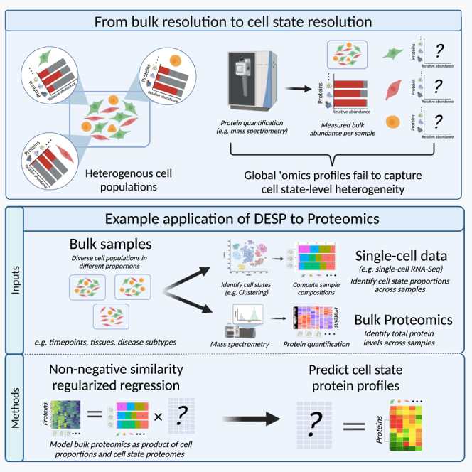
Overview of DESP algorithm

(A) Motivation and rationale behind DESP. Standard omic techniques such as mass spectrometry-based quantitative proteomics are often limited to bulk measurements of mixed cell populations and fail to resolve sample heterogeneity at the cell-state level.

(B) Analysis workflow. DESP takes as an input paired bulk omics data, e.g., proteomics, and matching single-cell data and predicts the contributions of the underlying cell states to the observed bulk measurements.

(C) Mathematical model. DESP models the observed bulk profiles, e.g., proteomics measurements, as the sum of unknown underlying cell-state profiles. DESP applies several constraints to this formulation to predict the unknown cell-state profiles.

(D) Output. Schematic of the DESP output showcasing its ability to demix and associate bulk sample measurements to the underlying contributing cell states for any given gene/protein.

Advances in single-cell molecular profiling, most notably single-cell RNA sequencing (scRNA-seq), offer a powerful approach for the identification and characterization of heterogeneous cell states in dynamic biological processes, such as cell differentiation and tissue development, leading to breakthroughs in emerging domains of biomedical research.^6,7 Related computational methods can define the quantitative transcriptomic profiles underlying these discrete cell states.⁸ However, these transcriptomic profiles have not proven to be accurate predictors of the corresponding protein expression patterns due to multiple biological and technical factors that lead to poor correlation between the cognate mRNA and protein levels of genes, preventing accurate inference of protein abundance using gene expression values such as those derived from scRNA-seq.^9,10,11 This represents an important gap in our understanding of the specialized molecular programs that define cell states in heterogeneous biological contexts.

As a generalizable computational solution to this challenge, we present a novel demixing algorithm titled DESP (Demixing Cell State Profiles in Bulk Omics) that leverages information on cell-state proportions derived from single-cell techniques to deconvolute standard bulk proteomics measurements of heterogeneous cell mixtures by distinguishing the underlying contributions of the involved cell states. DESP’s mathematical model is designed to circumvent the poor mRNA-protein correlation, which represents a major challenge for multi-omics integration efforts, by leveraging the ability of single-cell readouts, such as scRNA-seq or fluorescence-activated cell sorting (FACS), to identify the proportions of distinct cell states within dynamic heterogeneous samples for which bulk proteomics measurements were generated. DESP’s model combines these observed changes in cell-state proportions with the corresponding variations in bulk-level protein abundance to estimate the relative protein abundance levels associated with each cell state. While we demonstrate DESP’s utility using proteomics data in this paper, it can be applied to demix any type of bulk omics data, such as metabolomics or phopshoproteomics.

We applied DESP to a multi-omics time course dataset investigating the molecular changes of pre-cancerous cells undergoing transforming growth factor (TGF)-beta-induced epithelial-to-mesenchymal transition (EMT) in vitro.^12,13 EMT is a complex biological process by which epithelial cells lose their adhesion and gradually differentiate into mobile mesenchymal cells and is of particular importance to the biomedical community due to its integral role in wound healing, tissue development, and cancer progression.¹² We analyzed bulk quantitative proteomics and scRNA-seq data generated at eight consecutive time points representing MCF10A mammary epithelial cells undergoing EMT,¹³ and we show that DESP is able to identify the corresponding cellular proteomes and recover expected patterns of canonical EMT markers. Additionally, DESP goes further by identifying the proteomic profile of transient cell states key to the differentiation process that were not detected at the transcriptomics level and whose signal is significantly diluted in the bulk proteomics due to the confounding presence of other cell states in the mixture. These results demonstrate a compelling use case of DESP while also shedding light on the transient nature of intermediate molecular mechanisms driving EMT.

Results

DESP algorithm overview

DESP is a tool for deconvoluting bulk omics data to the cell-state level by estimating the contributions of the underlying cell states to the observed bulk measurements. Figure 1B shows an overview of DESP as applied to proteomics data as an example. DESP combines bulk proteomics data with single-cell data, such as scRNA-seq, acquired for a set of biological samples representing different physiological contexts. Examples of potential applications for DESP include time course experiments, cross-tissue omics atlases, or studies comparing disease subtypes. The single-cell data is used solely to delineate the proportions of the cell states that make up the samples under study and, optionally, their quantitative similarities to each other. The resultant cell-state composition matrix is fed into DESP alongside corresponding bulk protein measurements (Figure 1C), where the objective is to find the most likely possible combination of cell-state-level protein abundances whose sum would lead to the observed bulk measurements. The output of DESP is a matrix containing the predicted protein levels for each of the pre-defined cell states, effectively demixing the measured bulk proteomics matrix into the underlying cell-state proteomes (Figure 1D).

The premise of DESP is that the bulk proteome can be modeled as the sum of the underlying single-cell proteomes. Near-complete sequencing coverage of current single-cell technologies like scRNA-seq make it routinely feasible to obtain the identity and proportions of cell states in given biological samples,^6,7 and advances in mass spectrometry make acquiring comprehensive measurements of bulk proteomes similarly feasible.^6,7 We thus sought to integrate these readily available and comprehensive data types within a computational framework that could predict the experimentally challenging single-cell proteomes. DESP achieves this goal by applying the bulk-as-sum-of-single-cells principle through modeling the measured global proteome as the product of the observed cell-state proportions and the unknown corresponding cell-state proteomes, providing a simple but effective formulation that can be solved mathematically to estimate the cell-state proteomes (Figure 1C).

The DESP model solves a typically under-determined problem where the number of samples is less than the number of cell states. For example, an experiment that surveys a handful of cancer subtypes will likely contain dozens of cell states involved, as such giving many possible cell-level proteomes that could lead to the observed bulk proteome. We thus apply a set of both biologically and mathematically motivated constraints to guide the algorithm toward the optimal solution in a deterministic manner (Figure 1C). One notable constraint leverages correlations between cell-state profiles in the input single-cell data to maintain the global cell-state structure within DESP’s predictions by preserving the original state-state similarities. Notably, DESP’s robustness to input parameters allows it to efficiently make predictions without requiring parameter tuning (Figure S1). A detailed description of the mathematical model can be found in the STAR Methods section.

DESP does not aim to define cell states or their proportions from omics data, but rather it predicts the proteome of pre-defined cell states of interest based on the bulk proteomics data. The utility of DESP thus lies in the presence of established routine workflows for identifying the global proteome and cell-state composition of heterogeneous samples, effectively bypassing the lack of methods for deep measurement of individual cell proteomes. It is worth noting that DESP is agnostic of the technique used to identify cell-state proportions and thus does not directly use the single-cell measurements to infer the protein levels of the given cell states, allowing DESP to avoid issues regarding poor correlations between different data types such as RNA-seq and proteomics.

Multi-omics profiling of EMT

We applied DESP to a time course study examining pre-cancerous cells undergoing TGF-beta-induced EMT.¹³ Bulk quantitative proteomics and scRNA-seq data for over 5,600 genes were generated in parallel for eight consecutive time points as MCF10A human mammary epithelial cells underwent the EMT differentiation process (Figure 2A). Analysis of the scRNA-seq data using the Seurat tool¹⁴ revealed ten discrete cell states among the 1,913 captured cells, with intermediate states emerging from the predominantly epithelial cultures before transforming into the mesenchymal end state over the time course (Figures 2C and 2D). The availability of both bulk protein measurements and single-cell proportion information for the samples along with the dynamic nature of the samples’ cellular compositions render it an excellent testbed for DESP (Figure 2F). This dataset was thus used for both algorithm validation and as a case study of a real-life application of DESP (Figures 2G and 2H).

Figure 2.

Case study: Epithelial-to-mesenchymal transition

(A) Case study: Epithelial-to-mesenchymal transition (EMT) dynamic multi-omics profiling. In this experiment, bulk proteomics and scRNA-seq data were generated for human MCF10A cells undergoing TGF-beta-induced EMT across eight consecutive time points, generating molecular profiles of transient intermediate states.

(B) Dynamic scRNA-seq profiles. Heatmap visualizes the scaled relative expression of genes (rows) across cells (columns).

(C) Identification of intermediate cell states occurring during EMT. Clustering the scRNA-seq data reveals ten intermediate cell states as visualized on UMAP plot.

(D) Cell-state fluctuations during EMT. Bar plot visualizing cell-state composition at each time point.

(E) Mass spectrometry-based quantitative proteomics profiles. Heatmap visualizes scaled TMT reporter ion intensity, a proxy for relative abundance, of proteins (rows) across time points (columns).

(F) Applying DESP to EMT bulk proteomic profiles and scRNA-derived cell-state composition matrix to predict cell-state-level protein profiles.

(G) Prediction of intermediate cell-state profiles using DESP. Heatmap visualizes the predicted relative protein abundances for each of the cell states. One putative marker of a transient cell state is highlighted as an example finding from these predictions.

(H) Identifying contribution of individual cell states to time point bulk proteomics measurements. Schematic shows DESP demixing of a given protein to distinct underlying cell states, highlighting a transient cell-state signal that is lost by examining bulk measurements alone due to the presence of confounding signals from multiple cell states within each time point.

Validation using “pseudobulk” RNA data

To validate the algorithm and assess performance, we investigated DESP’s ability to recover the RNA profiles of individual EMT cell states from corresponding bulk RNA profiles. We utilized the scRNA-seq data, and not the proteomics, for the mathematical validation, as they represent the “true” experimentally derived single-cell profiles to compare against DESP’s bulk-inferred predictions. Since DESP’s predictions are made at the resolution of cell states rather than single cells, we constructed representative cell-state profiles from the scRNA data by averaging the expression of each gene in each cell state’s cells to represent the ground truth.¹⁵ Figure 3A shows a schematic illustrating the validation strategy, where a pseudobulk RNA matrix is first created by summing the scRNA measurements within each of the eight time points. We then used DESP to demix these pseudobulk profiles to the level of the ten cell states present in this dataset, as guided by the scRNA-derived changes in cell-state proportions across the time points (STAR Methods). These predicted cell-state profiles were then compared to the ground-truth profiles.

Figure 3.

Mathematical validation of DESP using pseudobulk RNA data

(A) Validation strategy. Pseudobulk profiles, generated by summing the scRNA profiles in each time point, were demixed by DESP guided by the cell-state compositions. The predicted DESP profiles were compared to the averaged per-cluster gene expression values in the input scRNA data.

(B) UMAP showing overlap of the real and predicted cell-state profiles, labeled as “centroids,” within the global structure of the scRNA-seq data.

(C) Bar plots showing the average Euclidean distance between each cell state’s constituent single-cell measurements to their real centroid compared to that of the predicted centroid.

(D) Mapping predicted centroids to the closest real centroid based on solving the linear sum assignment problem to minimize total Euclidean distances.

(E) Relative per-gene prediction error when varying the number of cell clusters input to DESP, highlighting the chosen 10 cluster scenario. Standard error bars are not visible due to small error range.

(F) Relative per-gene prediction error when systematically introducing noise to the input cell cluster proportions. The noise is introduced as relative deviations from the true cell proportions matrix.

Several metrics were used to compare the real and predicted cell-state profiles, henceforth referred to as “centroids,” to determine whether DESP’s predictions were reasonable approximations of the ground truth. To visualize the similarity of the predicted and real centroids within the global structure of the single-cell data, we created a uniform manifold approximation and projection (UMAP) projection of the scRNA data with the centroids overlayed, showing strong overlap between the real and predicted centroids (Figure 3B). We also quantitively assessed DESP’s ability to recover the true centroids by computing the average Euclidean distance between each state’s constituent single-cell measurements to their real centroid compared to that of the predicted centroid, again showing that the predictions fall within the correct intra-cell-state range (Figure 3C). Mapping the real and predicted centroids in a one-to-one manner based on minimizing their Euclidean distances showed that DESP correctly assigned centroid labels with a near-zero total distance (Figure 3D). Additionally, the mean per-gene relative prediction error was only 15% (interquartile range [IQR] 6%–17%), suggesting reasonable approximations of the real data even down to the level of individual genes (Figure 3E).

Accurate estimation of cell proportions from molecular profiling data is crucial in understanding the cellular composition of complex tissues, but experimentally determined proportions often deviate from the true underlying ones. To assess the impact of errors in user-provided cell-state proportions on DESP’s predictions, we systematically introduced random errors to the true matrix, ranging from 5% to 50% in increments of 5% (STAR Methods). This introduced variability in the cell-state proportions, mimicking real-world experimental uncertainties. The results reveal a nuanced relationship between the level of noise and the performance of DESP (Figure 3F). At lower levels of noise up to 25%, only a slight increase in prediction error (2%–3%) was observed. Interestingly, the algorithm demonstrated a more noticeable decrease in performance beyond this threshold but remained within 10% of its original prediction errors even when subjected to up to 50% introduced noise.

Cell-state assignments by tools such as Seurat can be imprecise. Hence, to ensure the robustness of DESP to variations in the number of input cell states, we repeated the validation with numbers of input cell states varying between 5 and 20 and found that while the prediction error expectedly increased with the number of states, it remained within a modest error range (Figure 3E). We also show that DESP is robust to a wide range of its two input parameters, with negligible effects on performance (Figure S1).

Since DESP performs predictions on a feature-by-feature basis, we also examined whether the accuracy of predictions varied with the expression of particular genes and observed that more cross-cell stable “housekeeping” genes had lower prediction errors than the more variable genes, while expression magnitudes were not influential (Figures S2A and S2B). In a similar vein, we examined the relationship between the prediction errors and cell-state properties and found that the larger and more homogeneous states had the lowest prediction errors (Figure S2C).

Validation using the Human Cell Atlas

To further validate the effectiveness of DESP, an additional case study was conducted using scRNA-seq data obtained from the Human Cell Atlas.¹⁶ The Human Cell Atlas provides a comprehensive collection of scRNA-seq data, encompassing 48,852 genes expressed across 24 human tissues. This dataset serves as a global reference atlas of human cell expression profiles, offering an ideal opportunity to assess DESP’s performance on large-scale datasets (Figure 4A).

Figure 4.

Benchmarking DESP using Human Cell Atlas and CITE-seq data

(A) UMAP plot visualizing the Human Cell Atlas scRNA-seq data color coded by cell type.

(B) Bar plot visualizing cell-type composition of the 24 tissues from the Human Cell Atlas database.

(C) UMAP plot showing overlap of averaged cross-tissue cell-type profiles as computed from the original scRNA-seq data and as predicted by DESP. Lines connect the points corresponding to the real and predicted profiles of the same cell type.

(D) Histogram showing distribution of DESP-relative prediction errors for each of the 48,846 genes from the Human Cell Atlas database.

(E) Histogram showing distribution of DESP-relative prediction errors for each of the 36 cell types from the Human Cell Atlas database.

(F) (Left) UMAP plot visualizing the CITE-seq single-cell data color coded by cell type. (Middle) Bar plot visualizing cell-type composition of samples. (Right) Boxplot comparing DESP’s per-gene relative prediction error for the RNA and protein data separately.

For the validation process, we focused on the 36 most prevalent cell types, as determined by the number of tissues in which each cell type was present. Initially, we constructed a matrix that represented the proportion of each cell type within each tissue (Figure 4B). Subsequently, we evaluated DESP’s ability to reconstruct the single-cell profiles by applying it to a pseudobulk dataset. This dataset was generated by summarizing the scRNA-seq data at the tissue level by averaging the expression of each gene within each cell type and multiplying these averaged expressions by the corresponding cell-type proportions across tissues (STAR Methods).

We performed a qualitative evaluation of DESP’s performance by combining the real and predicted cell-type profiles into one matrix and constructing a UMAP plot that visualizes these profiles in two dimensions, revealing strong overlap between the corresponding real and predicted cell-type profiles within this reduced dimensional space (Figure 4C). As a quantitative assessment, we computed the relative prediction error on a gene-by-gene basis by summing the absolute difference between each gene’s real and DESP-predicted averaged cell-type profiles divided by the real cell-type profiles. The resultant median per-gene error was 15%, and the mean was 20% (IQR 6%–30%) (Figure 4D). We repeated the same analysis for each cell type separately, finding a median per-cell-type error of 7% and a mean of 10% (IQR 2%–13%) (Figure 4E). In our experiment, it took only 6 s to perform the demixing for all 48,852 genes on a standard laptop machine, demonstrating DESP’s ability to swiftly produce accurate predictions on large-scale datasets.

Performance comparison between transcriptomics and proteomics

DESP provides a mathematical framework for charting the relationship between single-cell and bulk omics datasets, which depends on the assumption that the bulk data can be modeled as the sum of the single-cell data. To ensure that this relationship holds for different types of omics data, we performed mathematical validation using both single-cell transcriptomics and proteomics datasets as described in the corresponding sections of this paper. Furthermore, to test the scenario where both datasets were obtained from the same samples, we applied DESP to matched single-cell transcriptome and protein data generated by the cellular indexing of transcriptomes and epitopes (CITE)-seq technology from the Hao et al. study.¹⁷ This dataset comprised 161,764 peripheral blood mononuclear cells (PBMCs)isolated from 8 individuals at three time points after receiving an HIV vaccine. The authors grouped the cells into 31 annotated immune cell types. Notably, there were 187 genes that had both RNA and protein measurements available for analysis.

We used DESP to independently demix two pseudobulk datasets created using the same underlying cell-type composition matrix: the aggregated RNA data and the aggregated protein data per sample (STAR Methods). Comparing the 31 DESP-predicted cell-type profiles to the true ones measured by CITE-seq revealed a median per-gene relative prediction error of 27% (IQR 21%–34%) for the protein data compared to 46% (IQR 28%–70%) for the RNA data (Figure 4F). These results indicate that DESP can predict single-cell protein measurements from transcriptomics-derived cell-type structures with comparable, or even superior, accuracy to its predictions for transcriptomics data. These observations align with previous research highlighting the consistency of high-level cell-type assignments between RNA and protein measurements, despite the discordance in per-gene correlations between RNA-seq and proteomics data.^5,17

Comparison with experimentally derived profiles

We applied DESP to demix the EMT dynamic bulk proteomics data by separating the contributions of the ten cell states to each of the eight time point bulk measurements, revealing the underlying proteome profiles of the cell states (STAR Methods). To benchmark these predicted protein profiles, we analyzed single-cell proteomics data from an analogous model of EMT generated by the SCoPE2⁴ platform, which quantified >1,700 proteins across 420 cells at three key transition time points.¹⁸ The similarity of this independent experimental model to our EMT multi-omics case study combined with the presence of more than 1,000 overlapping proteins between them make it ideal for comparing DESP’s computationally predicted protein profiles to independently acquired, experimentally derived ones.

We first used a k-nearest neighbor strategy to impute missing values in the single-cell proteomics data followed by clustering the cells (STAR Methods). The clusters in both datasets were labeled as epithelial (E), intermediate (I), or mesenchymal (M) based on their temporal dynamics and expression of canonical EMT markers (STAR Methods; Figure 5A). To mitigate potential confounding factors arising from technical experimental variations, our benchmarking strategy focused on the comparative analysis of the three EMT cell states (E, I, and M). Specifically, we assessed whether the protein fold changes inferred from DESP’s predicted profiles exhibited greater resemblance to the experimentally derived fold changes compared to those derived solely from the scRNA data (Figure 5B).

Figure 5.

Comparing DESP predictions to experimentally derived profiles

(A) Dynamic EMT single-cell proteomics data used for biological validation.

(B) Heatmap of computed protein relative abundance fold changes between cell states in single-proteomics data, scRNA data, and bulk-demixed DESP predictions.

(C) Pearson correlation of the protein relative abundance fold changes between cell states in each dataset. p values are based on Fisher’s z transformation of the Pearson correlation coefficients.

(D) UMAP plot showing overlap of the real and DESP-predicted cell-state profiles, labeled as centroids, within the global structure of the single-cell proteomics data. Inset plot: results of mapping each predicted centroid profile to the closest real centroid profile in a one-to-one manner based on solving the linear sum assignment problem.

(E) Bar plots showing the average Euclidean distance between each cell state’s constituent single-cell measurements to their real centroid compared to that of the DESP-predicted centroid.

For this benchmark, we selected the proteins with high correlation (Pearson R² > 0.5) between the bulk proteomics and a pseudobulk matrix constructed by summing the single-cell proteomics data in each time point to address technical variation between the single-cell and bulk proteomics measurements (STAR Methods). We also focused our comparison on the genes that differ the most (Pearson R² < −0.5) between the bulk proteomics and pseudobulk scRNA, representing the genes that are the best at distinguishing the RNA and protein levels in these data and thus are appropriate for benchmarking DESP. By computing the Pearson correlation between the resulting fold changes, we observed that DESP’s predictions not only exhibited significant correlation (p < 0.05) with the single-cell proteomics data but were also significantly closer to the single-cell proteomics fold changes compared to the scRNA-derived fold changes, suggesting that DESP’s predictions align well with the experimentally derived profiles (Figure 5C).

As an additional validation of DESP’s performance with proteomics data and the consistency of the bulk-single cell relationship across the protein and RNA layers, we also created a pseudobulk proteomics matrix by summing the experimentally derived single-cell proteomics profiles within each time point. We then used DESP to demix these per-time point pseudobulk profiles to the level of the identified cell states, guided by the single-cell-derived changes in cell-state proportions across the time points. We used the same input parameters used for applying DESP to the transcriptomics data (λ = 1⁻⁷, β = 1⁻⁴). These predicted cell-state profiles were then compared to the true cell-state profiles obtained from the single-cell proteomics data by averaging the relative abundance of each protein in each cell state. The average per-protein relative prediction error was only 2.7% (IQR 0.5%–3.8%), and the cell-state-level results visualized in Figures 5D and 5E quantitively and qualitatively demonstrate the ability of DESP to accurately recapture the real cell-state profiles from the pseudobulk quantifications. Put together, these results demonstrate the generalizability of DESP and the potential for applications to other types of omics data without need for custom configurations.

Detection of transient EMT mechanisms using DESP

Applying DESP to demix the bulk EMT proteomics profiles allowed us to contextualize the cross-time point proteome changes according to the underlying cell states and to characterize the distinct protein programs that occur during EMT that are lost in the bulk measurements, as elaborated upon below.

To evaluate the extent to which DESP’s predictions provided information beyond what the bulk proteomics or scRNA data provided alone, we compared the results of performing differential expression analysis between the cell states from the DESP predictions versus those two original data types by themselves and found that DESP detected hundreds of markers for the EMT stages that were not deemed differential in the other techniques (Figure S3). Several of these markers are known to be involved in EMT, such as TPM2 in the E state and CD44 in the M state.

Gene set enrichment analysis also revealed more than 200 pathways that were significantly enriched among DESP-identified markers but not revealed by the other standard approaches, demonstrating DESP’s ability to glean novel insight into the involved molecular mechanisms rather than just recapitulating what existing methods would have found (Figure 6A). These pathways included both canonical EMT-related pathways such as signaling, migration, and wound healing, as well as potentially novel biological processes that had not been associated with EMT before, such as cellular stress response, spliceosome assembly, and protein transport (Figure 6B).

Figure 6.

Detection of transient EMT mechanisms using DESP

(A) Venn diagrams showing overlap of significantly enriched pathways within each EMT stage detected by scRNA-seq data alone, bulk proteomics data alone, and DESP predictions.

(B) Heatmap of relative enrichment scores of selected GO terms among cell-stage markers that were enriched among DESP’s predictions compared to results obtained from scRNA-seq or bulk proteomics alone.

(C) PRC2 core histone methylation complex. The EZH2 and H2AFX proteins are highlighted based on their inferred influential transient profiles detected by DESP.

(D) DESP demixing of H2AFX across transient cell states, with intermediate time point T2 highlighting the time-sensitive disproportionate contribution by transient cell state 8.

(E) Heatmap of temporal phosphorylation of EZH2 and H2AFX in global quantitative phosphoproteomics analysis of the same EMT samples.

The intermediate cell states are of high interest due to their transient nature and expected influential role in driving EMT. We thus sought to investigate if unique insights could be gleaned by DESP on the transient molecular mechanisms governing EMT. Notably, eight proteins, including three encoded by histone genes, were identified as being key to the transition due to their relative enrichment in the predicted intermediate cell-state proteome compared to their diluted signal in the bulk proteomics data, representing a signal that likely would have been missed if analyzing bulk proteomics alone (Figure 6D).

Of these eight proteins, H2AFX stands out as a marker (99th percentile) of the predicted intermediate proteomics profile yet with low abundance (9th percentile) in the corresponding scRNA profile, suggesting extensive post-transcriptional regulation. H2AFX is a core histone protein variant that both contributes to chromatin remodeling and is post-translationally modified during EMT.^19,20 Notably, H2AFX is hyper-phosphorylated during the earliest time points of EMT,¹³ suggesting a change in this protein’s functional activity during the initial intermediate cell states (Figure 6E).

The STRING database²¹ shows that H2AFX and two other DESP-identified markers are functionally linked with nine proteins annotated as EMT associated in the GO²² and MSigDB Hallmark gene sets.²³ One of these associated proteins is EZH2, which is part of the PRC2 chromatin remodeling complex that performs transcriptionally inhibitory histone methylation (Figure 6C). EZH2 has emerged in recent years as a promising target for cancer treatments,^24,25 with an FDA-approved drug (tazemetostat) targeting EZH2 as a cancer treatment²⁶ and another EZH2-targeting compound currently in clinical trials.²⁷ In contrast to its target H2AFX, EZH2 shows elevated phosphorylation during later time points of the experiment, suggesting the activation of a delayed regulatory “switch” after 3 days of TGF-beta induction.

Taken together, these findings generated by DESP-based proteomic demixing pinpoint specific transient events as plausible mechanisms governing EMT progression despite the RNA-protein discord.

Discussion

Here, we present, evaluate, and apply DESP as an algorithm for resolving the contributions of cell states to quantitative global proteomics measurements and potentially other bulk omics profiles. DESP enables researchers to gain insights into dynamic cell-state contexts from standard bulk omics workflows, helping to integrate underserved omics layers like proteomics into the rapidly evolving single-cell analysis toolkit. We validated DESP mathematically and obtained independent experimental evidence supporting the validity of DESP’s predictions. We also applied DESP to tease out the proteome composition of transient intermediate cell states in an in vitro model of EMT, shining a light on key intermediate molecular mechanisms.

We note that as a new type of demixing algorithm, DESP does not aim to define, nor does it require, the optimal cell-state structures for the bulk data to be demixed. Rather, DESP solves the problem of mapping bulk omics measurements, such as proteomics, to a pre-defined cell-state structure of interest to the user, independent of how that structure was originally defined. In contrast to existing omics deconvolution algorithms,²⁸ DESP does not aim to predict cell-state proportions, but instead it predicts the proteome of given cell states based on demixing the bulk data. DESP also offers a generalizable framework applicable to all types of omics data unlike existing single-cell inference algorithms, such as TCA²⁹ and BMIND,³⁰ that are tailored to specific data types. DESP provides a generalizable computational framework for bulk omics demixing, with planned future applications including demixing protein interaction networks and spatial transcriptomics data. To facilitate adoption and usability by the community, DESP is available as an R package at https://github.com/AhmedYoussef95/DESP.

Limitations of the study

DESP is especially well suited for biological scenarios characterized by dynamic shifts in cell-state/-type composition across a range of samples, as exemplified in the presented case studies. However, its accuracy diminishes when applied to “static” biological contexts where cell proportions or the corresponding bulk omics measurements exhibit minimal changes. Notably, DESP’s performance is significantly influenced by the ratio between the number of cell states and the number of bulk samples in the system under study, displaying diminished accuracy when the former greatly exceeds the latter. Furthermore, DESP lacks the capability to handle missing values and address batch effects in input data and thus relies on the user to perform appropriate imputation and data pre-processing when necessary. Related to this, acknowledging that log transformation is a common pre-processing step for omics data, we recommend reversing log transformations before applying DESP to align with its additive model (bulk as sum of single cells), followed by log transformation of the resultant cell-state-level predictions for downstream analyses as needed.

STAR★Methods

Key resources table

REAGENT or RESOURCE	SOURCE	IDENTIFIER
Deposited data
Raw and analyzed data	This paper	https://doi.org/10.1101/2023.01.19.524460
Human Cell Atlas scRNA-seq data	Regev et al.16	https://doi.org/10.7554/eLife.27041
CITE-Seq single-cell proteomics and transcriptomics	Hao et al.17	https://doi.org/10.1016/j.cell.2021.04.048
EMT proteomics and scRNA-Seq data	Paul et al.13	https://doi.org/10.1038/s41467-023-36122-x
EMT single-cell proteomics data	Khan et al.18	https://doi.org/10.1101/2023.12.21.572913
Software and algorithms
DESP algorithm	This paper	https://github.com/AhmedYoussef95/DESP https://doi.org/10.5281/zenodo.10633315
STRING database	Szklarczyk et al.21	https://doi.org/10.1093/nar/gkaa1074
Gene Ontology (GO) database	GO Consortium23	https://doi.org/10.1093/nar/gkaa1113
MSigDB gene set collection	Liberzon et al.23	https://doi.org/10.1016/j.cels.2015.12.004
DrugBank database	Wishart et al.27	https://doi.org/10.1093/nar/gkx1037
OMIM database	Amberger et al.31	https://doi.org/10.1093/nar/gku1205
KEGG database	Kanehisa et al.32	https://doi.org/10.1093/nar/gkv1070
MaxQuant software	Tyanova et al.33	https://doi.org/10.1038/nprot.2016.136

Resource availability

Lead contact

Further information and requests for resources should be directed to and will be fulfilled by the lead contact, Andrew Emili (emili@ohsu.edu).

Materials availability

This study is purely computational and did not generate any unique reagents.

Data and code availability

• •All supporting raw and processed data along with the associated analysis scripts are publicly-available and can be found on Zenodo at https://zenodo.org/records/10345000 (https://doi.org/10.1101/2023.01.19.524460).
• •DESP is available as an R package with all original code and detailed documentation publicly-available at https://github.com/AhmedYoussef95/DESP. A persistent archived version of record of the repository is also publicly-available on Zenodo (https://doi.org/10.5281/zenodo.10633315).
• •Any additional information required to reanalyze the data reported in this paper is available from the lead contact upon request.

Method details

DESP algorithm

Background

We formalize DESP as recovery of cell state profiles under the mixing equation $AX=Y$, with mixing matrix $A$ (samples $\times$ states) applied to unobserved state profiles $X$ (states $\times$ genes) yielding observed bulk data $Y$ (samples $\times$ genes). Each pair of corresponding columns of $X$ and $Y$ is an independent equation; in what follows we denote a column of $X$ as $x$ and the corresponding column of $Y$ as $y$.

This problem is challenging when there are fewer samples than states, leading to an ill-posed linear inverse problem. To constrain the solution toward meaningful and biologically likely profiles, DESP applies a series of regularizations as described next.

Nonnegativity

First, DESP imposes nonnegativity on the solutions. This leads to the nonnegative least squares problem:

$$\hat{x}=\mathit{arg}\underset{x\ge 0}{\mathit{min}}{\Vert Ax-y\Vert }^2\text{.}$$

which is equivalent to the quadratic program:

$$\hat{x}=\mathit{arg}\underset{x\ge 0}{\mathit{min}}-2y^{T}Ax+x^T{A}^{T}Ax\text{.}$$

Tikhonov regularization

Next, DESP incorporates Tikhonov regularization (ridge regression) to favor small-norm solutions:

$${{\Vert Ax-y\Vert }^2+{\lambda }_x\Vert x\Vert }^2$$

We use the notation ${\lambda }_x$ to indicate that the proper amount of regularization can be chosen based on the properties of $x$. (As shown in Figure S2, statistical properties of individual gene expressions are correlated with estimation accuracy.) However, our results are based on using the same value of ${\lambda }_x$ for all genes. As shown in Figure S1, using a single value of ${\lambda }_x$ across all genes yields good recovery in general with results that are relatively insensitive to the specific value of ${\lambda }_x$ (chosen within a broad range).

Expressed as a quadratic program this becomes:

$$\hat{x}=\mathit{arg}\underset{x\ge 0}{\mathit{min}}-2y^{T}Ax+x^T\left(A^{T}A+{\lambda }_{x}I\right)x$$

Similarity regularization

Finally, we make the following observation: the process used to construct $A$ may have access to additional information. For example, when scRNA clusters are used to define the cell states leading to the cluster mixtures in $A$, DESP can extract useful information from the cluster RNA expression profiles. We emphasize that this information can be useful even though no assumption is made about any particular relationship between, for example, RNA expression levels and protein abundance. DESP employs this strategy by incorporating a state-state similarity measure. While in principle DESP can use any similarity or dissimilarity matrix, in our results DESP operates using scRNA data as follows:

Define the matrix $C$ to consist of cell state profiles with cell state profiles on the rows and genes on the columns, where entries in $C$ correspond to average gene expression in the cell state. (Processing of scRNA data to form cell state profiles is discussed below.) Rows of $C$ are standardized to zero mean and unit norm, to obtain $\tilde{C}$, which is used to form the correlation matrix of clusters

$$M=\tilde{C}{\tilde{C}}^T$$

$M$ is typically invertible due to the independence of cell states, so DESP performs similarity regularization by seeking to minimize $x^T{M}^{-1}x$

Hence to include cell state similarity as a form of regularization, DESP minimizes:

$$\hat{x}=\mathit{arg}\underset{x\ge 0}{\mathit{min}}\Vert Ax-y{\Vert }^2+{\lambda }_x\Vert x{\Vert }^2+\beta x^T{M}^{-1}x$$

which is equivalent to the quadratic program:

$$\hat{x}=\mathit{arg}\underset{x\ge 0}{\mathit{min}}-2y^{T}Ax+x^T\left(A^{T}A+{\lambda }_{x}I+\beta M^{-1}\right)x\text{.}$$ (Equation 1)

As for ${\mathit{\lambda }}_{\mathit{x}}$, we find that DESP obtains good recovery in general for $\mathit{\beta }$ values across a fairly broad range (Figure S1).

Implementation

The R function solve.QP from the quadprog package can solve any of the above quadratic programs. So for each feature (e.g., gene/protein), DESP invokes solve.QP to solve the constrained minimization (1) to estimate cell state profiles. DESP also has minimal running time; in our experiments, we found that DESP performed predictions for >8,000 features within less than a second on a standard laptop machine.

Robustness to noise in user-provided cell state proportions matrix

We systematically introduced noise to a cell state proportions matrix to assess the DESP algorithm’s stability and robustness to variations in the user-provided cell state proportions matrix. As described in the section 'identifying intermediate cell states from scRNA-Seq data", we generated a cell state proportions matrix representing the cell state composition of the 10 different EMT cell states across the 8 timepoints profiled in that experiment. This matrix served as our ground truth proportions matrix. We also constructed a ‘pseudobulk’ matrix representing the summed gene expression levels across all cell states within each timepoint, representing our ground truth bulk data, along with the ground truth averaged expression profiles of each cell state. We systematically introduced random noise to the proportions, ranging in increments of 5% from 5% to 50% of the original values, by drawing multiplicative noise values from a uniform distribution and subsequently normalizing them to ensure cumulative alignment with the selected noise level. For each noise level, we computed DESP’s relative per-gene prediction error for demixing the same pseudobulk matrix to predict the cell state expression profiles. We repeated this experiment 1,000 times for each noise level to account for the random nature of noise generation and ensured reproducibility by setting a seed for the random noise generation. The averaged prediction error for each noise level provided a nuanced understanding of DESP’s behavior in response to input variations and contributed valuable insights for its practical application in noisy biological datasets.

Testing robustness of DESP predictions with different numbers of cell states

In the EMT case study detailed in the manuscript, we identified ten transitional cell states occurring during EMT. These cell states were identified by clustering the single-cell RNA-Seq data to reveal groups of transcriptionally-correlated cells using the Seurat R package (STAR Methods). Since determining the optimal number of cell states form scRNA-Seq data is not an objective process, we repeated our mathematical validation of DESP using different numbers of input cell states to examine the robustness of DESP’s predictions.

To vary the number of cell states, we used different clustering resolutions within Seurat’s FindClusters algorithm followed by repeating the process for constructing a cell state proportions matrix detailing the proportion of each cell state within each of the timepoints. We tested DESP using numbers of clusters varying between 5 and 20 and computed mean per-gene relative prediction error for each case (Figure 3E). For cases where there were 8 or less cell states, the problem was overdetermined due to the presence of eight timepoints in the data and thus the prediction error was zero. Starting from nine clusters and above, the problem is underdetermined meaning that multiple possible combinations of cell state protein profiles could lead to the observed pseudobulk measurements. As expected, we found that the prediction error increased as the number of cell states increased, with the error ranging from 10 to 25% for cases with 9–20 clusters respectively.

Testing robustness of DESP predictions to input parameters

DESP expects two input parameters denoted as λ and β (STAR Methods). In the EMT case study described in the manuscript, we set the values of these parameters to 1⁻⁷ and 1⁻⁴ respectively. To test the robustness of DESP’s predictions to variations in the values of the input parameters, we repeated the mathematical validation of DESP using combinations of the input parameters ranging from 1⁻¹⁰ to 1¹⁰, with increasing steps of an order of magnitude each, for each of the two parameters and quantified the mean per-gene relative prediction error for deconvoluting the scRNA-Seq ‘pseudobulk’ data (Figure S1).

We found that the error remained stable at 15% for a wide range of combinations of the input parameters, with predictions made with values of β ranging between 1⁻⁷ and 0.01 and corresponding values of λ of the same or less value all giving nearly identical results with errors of 15%. Furthermore, the error never exceeded 22% for any combination of the parameters with values between 1⁻¹⁰ and 1 for each parameter. The prediction errors were smaller for deconvoluting the pseudobulk single-cell proteomics data (Figures 5D and 5E), with prediction errors at 2% for any value of β between 1⁻¹⁰ and 0.1 and a corresponding λ of the same or less value, and never exceeding 16% for any combination of values between 1⁻¹⁰ and 1 for either parameter. These results demonstrate the robustness of DESP to variations in the input parameters and that there is no need to hypertune the input parameters for different input datasets.

Effect of gene/protein and cell cluster properties on DESP’s predictions

DESP performs predictions on a feature-by-feature basis. Depending on the input data, these features will typically be genes or proteins. We examined the correlation between mathematical properties of the features in the bulk data and their corresponding prediction error based on applying DESP to the scRNA-derived pseudobulk matrix as described in the mathematical validation chapter of the STAR Methods section. To explore the relationship between properties of the genes and their corresponding predicted values, for each of the 8,528 genes in the dataset we computed the following measures.

• (1)Expression specificity: This metric looked at the relative specificity of a given gene’s expression to the clusters. The coefficient of variation (CV) of the gene’s cluster-specific expression values is computed as the standard deviation of the per-cluster expression values divided by their mean. Genes with a lower CV can be interpreted as being relatively stable ‘housekeeping’ genes due to the smaller variance in their expressions across clusters.
• (2)Average expression: This metric is concerned with the relative quantity of each gene’s transcripts and is simply computed as the mean expression of the gene across clusters.

Each of the above properties was correlated to the gene’s relative prediction error, defined as the absolute difference between the real and predicted per-cluster values divided by the real value. A Pearson correlation coefficient of 0.6 was observed between the per-gene prediction errors and their expression specificity, indicating that the less variable ‘housekeeping’ genes tended to have higher prediction accuracy (Figure S2A). Meanwhile, the Pearson correlation coefficient was only (−0.01) with the genes’ average expression values, suggesting that the magnitude of a gene’s expression is less influential to DESP’s predictions (Figure S2B).

In a similar vein, we computed the Pearson correlation coefficient between the following mathematical properties of the cell clusters and their corresponding prediction errors measured as the Euclidean distance between the predicted centroids and the real ones.

• (1)Cluster heterogeneity: For each cluster, the average Euclidean distance between each member cell’s scRNA expression profile and that of its corresponding cluster centroid, i.e., the average expression profile of all cells belonging to the cluster.
• (2)Cluster size: The number of cells within each cluster.
• (3)Cluster fluctuation across samples: The coefficient of variation of each cluster’s proportion in each timepoint.

We found a positive correlation between cluster heterogeneity and the prediction error (Pearson R² = 0.48) indicating that the prediction error was lower for the more homogeneous clusters, a negative correlation with size (Pearson R² = −0.47) suggesting better prediction for larger clusters, and near-zero correlation with cross-sample cluster fluctuations (Pearson R² = 0.04) (Figures S2C–S2E). These results are potentially confounded however by the fact that cluster size and heterogeneity were strongly negatively-correlated to each other (Pearson R² = −0.65).

Quantification and statistical analysis

EMT multi-omics experiment summary

We used data from (Paul et al.).¹³ In that study, cells of the human mammary epithelial cell-line MCF10A were treated with TGF-Beta to induce epithelial-to-mesenchymal transition (EMT) and samples were aliquoted at ten timepoints for multi-omics profiling. Details on the experiment and the downloadable datasets can be accessed at (Paul et al.).¹³ Relevant data is also provided in the data and code availability section.

Proteomics data processing

Quantitative profiles of 6,967 proteins were generated by nanoLC-MS/MS across ten timepoints (0, 4 h, 1–6, 8 & 12 days post-TGF-Beta injection) with three biological replicates per timepoint. Raw MS files were processed using MaxQuant (version 1.6).³³ Tandem mass spectra were searched against the reference proteome of Homo sapiens (Taxonomy ID 9606) downloaded from UniProt in April 2017. Peptides of minimum seven amino acids and maximum of two missed cleavages were allowed, and a false discovery rate of 1% was used for the identification of peptides and proteins. Contaminants and reverse decoys were removed prior to downstream analysis. The average intensity across replicates was computed for each protein in each timepoint for downstream analysis. Timepoints 3 and 9 were not used in this study since they are not present in the scRNA-Seq data generated from these samples and subsequently used in downstream analysis. All data pre-processing of the MaxQuant files was performed using the R statistical software (version 4.1.0).

Single-cell RNA-Seq data processing

Single-cell RNA-Seq quantified the expression of 9,785 genes in 1,913 cells at eight consecutive timepoints, with roughly 200 cells per timepoint. Details on the experiment and the downloadable data can be found at (Paul et al., 2023).¹³ Low-quality genes detected in less than 5% of all cells were discarded (17 genes). Lowly-expressed genes with less than three counts in at least three cells were also removed (1,240 genes). On average, each cell expressed ∼3,600 genes after filtering. Finally, the data was normalized such that each cell’s expression values sum to one. Since DESP ultimately combines information derived from the scRNA-Seq data with the proteomics data, we filtered the scRNA-Seq data to the set of 5,606 genes for which quantitative bulk protein measurements were also present in this dataset for the identification of co-expressed cell states prior to applying DESP to the proteomics data. All processing of the scRNA-Seq data was performed using the R statistical software (version 4.1.0).

Identifying intermediate cell states from scRNA-seq data

The cell states in the dataset were identified in an unsupervised manner based on the similarity of gene expression profiles in the scRNA-Seq data. All 1,913 cells from all the timepoints were pooled together for this analysis. The Seurat¹⁴ R package was used to identify the cell states using their recommended workflow as follows. The data was normalized by dividing the gene counts in each cell by the total counts in the cell and multiplied by a scale factor of 10,000. The normalized counts were log-transformed after adding a pseudocount of one. The data was then centered by subtracting each gene’s expression by its average expression and scaled by dividing the centered expression levels by their standard deviations. The top 2,000 most variable genes were used to perform PCA dimensionality reduction and subsequently construct a k-nearest neighbor graph with k = 20 and 10 principal components used. Finally, the data was clustered using Seurat’s FindClusters function with a resolution of 1.1, defining ten co-expressed cell clusters ranging in size from 68 to 303 cells. The choice of ten clusters was made based on manual evaluation of the clustering results at different clustering resolutions. Table S1 contains information on the markers enriched among each of these identified clusters. In the rest of the manuscript, we use the term ‘cell states’ to refer to these ten clusters.

A matrix containing the cell state profiles (denoted ‘X’) was constructed by averaging the expression of each gene in each cell state. A cell state proportions matrix (denoted ‘A’) was also constructed by counting the number of cells from each state in each timepoint. These matrices were used in the downstream validation and application of DESP to the EMT multi-omics data. We also tested our approach on different pre-defined numbers of states ranging between five and fifteen by varying the clustering resolution to examine the effect of varying the number of cell populations on DESP’s predictions (Figure S1).

Each of the ten states identified in the previous step were also classified into one of three EMT stages based on their change in proportions across time: Epithelial (E), Mesenchymal (M), or Intermediate (I). The cell states with their maximum count in the earlier timepoints were labeled E, those in the later timepoints were labeled M, and those in the middle timepoints being I.

The following classifications were assigned.

• (1)Epithelial states: 2, 5, 9
• (2)Intermediate states: 8
• (3)Mesenchymal states: 7

Any cell states not included in the above list were deemed not to show a distinct cross-timepoint change in proportion pattern that would best fall into one of the three biological states of interest.

Validation using RNA pseudobulk

Prior to making inferences from the proteomics data, we first investigated DESP’s ability to recover the scRNA data from the bulk data at the RNA-level where we have the true single-cell profiles to compare against. To represent the bulk data that DESP expects as an input, we constructed a ‘pseudobulk’ matrix representing the summed gene expression levels across all cell states within each of the eight timepoints. This matrix is constructed as the product of multiplying the cell state proportions matrix ‘$\mathit{A}$’ and the cell state profile matrix ‘$\mathit{X}$’. The resultant matrix ‘$\mathit{Y}$’ had one value per gene in each timepoint. The cluster similarity matrix ‘$\mathit{M}’$ was created by computing the Pearson correlation between each pair of cell state profiles, i.e., the rows of the matrix ‘$\mathit{X}’$, and used to guide the algorithm toward a solution that preserves the relationship between the input cell states. We then use DESP to solve the under-determined problem $\mathit{Y}=\mathit{A}\mathit{X}’$ to predict the cell state profile matrix $\mathit{X}’$ as described in the ‘DESP algorithm overview’ section. Finally, the predicted cell state profile matrix $\mathit{X}’$ is then compared to the real cell state profile matrix $\mathit{X}$ to assess DESP’s performance. We utilized four different methods of assessing the prediction accuracy, each of which is detailed below.

We computed the mean per-gene relative absolute error between $X$ and $X’$ by calculating the absolute difference between each gene’s real cross-state expression values in $X$ and the predicted ones in $X’$ and taking the mean across all such gene-level errors. This metric was motivated by the fact that DESP performs its predictions independently for each gene. This metric was also used to evaluate the robustness of DESP to variations in its two input parameters λ and β by examining the results for different values of the parameters (Figure S1).

As a visualization of the similarity of the predicted profiles in $X’$ to the real ones in $X$ within the global structure of the single-cell data, we created a UMAP projection using the R package uwot on the original scRNA-Seq gene expression matrix with the addition of the real and predicted cell state profiles, i.e., the rows of $X$ and $X’$. The profiles were labeled on the subsequent UMAP plots to distinguish them from the individual cells (Figure 3B).

To determine if DESP’s predictions are reasonable approximations of the real data, we also compared the predictions to the real data by computing the Euclidean distance between individual cells’ measurements and their real state average as opposed to the distance between thee predictions and the same state average. More specifically, we iterated over each of the 1,913 cells in the original single-cell expression matrix and computing the Euclidean distance between the cell’s profile and that of its cell state’s profile. Next, for each cell state we compute the average distance of its cells to the averaged cell state profile, as well as the distance between the predicted profile and the same corresponding cell state profile. We then created bar plots comparing these two distances side-by-side to determine whether the predicted profiles fall within the correct intra-state range (Figure 3C).

Finally, we mapped the predicted cell state profiles to the real ones by solving the linear sum assignment problem (LSAP) using the Hungarian method as implemented in the solve_LSAP function in the clue R package³⁴ (Figure 3D). In summary, the LSAP algorithm expects similarities between cell state profiles as the entries in the input matrix. The idea of the matching is that given two sets A and B, we find the matching that maximizes $\text{sum}\left(\text{similarity}\left(\mathrm{a}\_\mathrm{i},\mathrm{b}\_\mathrm{j}\right)\right)$ where $\mathrm{a}\_\mathrm{i}$ is matched with $\mathrm{b}\_\mathrm{j}$, and each member of the set is matched with exactly one member of the other set. The algorithm was run twice; once with the Euclidean distance as the similarity metric for the state profiles where the algorithm minimized the sum of assigned Euclidean distances, and once with the Pearson correlation as the similarity metric where the algorithm maximized the summed correlations across cell state assignments.

Applying DESP to demix EMT bulk proteomics data

We used DESP to demix the EMT bulk proteomics data down to the level of the ten scRNA-defined cell states as described in the ‘DESP algorithm overview’ section. The inputs to DESP were the processed protein-by-timepoint proteomics matrix, the cell state proportions matrix indicating the proportion of each cell state in each timepoint, and the cell state similarity matrix containing the Pearson correlations between the cell state scRNA profiles. The parameters λ and β were set to 1⁻⁷ and 1⁻⁴ respectively based on the tuning results obtained from demixing the ‘pseudobulk’ as described in the previous section. The output was a protein-by-state matrix which was used for the analysis described in the results section of the manuscript.

Identifying cell state markers

The R package Seurat’s¹⁴ FindMarkers function was used to find the genes that distinguish each cell state in the scRNA-Seq data based on a one-vs-all differential expression analysis. An FDR cutoff of 0.05 and log fold-change cutoff of 0.5 were applied to determine the marker genes for each state. These markers are listed in Table S1. This analysis was performed once at the level of the ten individual cell states, to confirm the classification of the cell states into the E/I/M stages, and once at the level of the three stages for pathway enrichment and comparing marker genes across datasets. This analysis identified 142 marker genes for the E state, 36 for the I state, and 81 for the M state in the scRNA-Seq data (Table S2). For the predicted cell state proteomics profiles from DESP, since we have only one measurement per cell state as opposed to the multiple per-cluster cell measurements in the scRNA-Seq data, we define the marker proteins for each cell state as those with an average log2 fold-change greater than 1 between each state and the average of all the other ones (Table S1). As with the scRNA-Seq data, this analysis was repeated for the three EMT stages (E, I, and M) instead of the ten cell states after the initial cell states were classified into each of the three stages. This identified 90 marker proteins for the E state, 215 for the I state, and 155 for the M state in the DESP predictions (Table S2).

Identifying timepoint markers in bulk proteomics

We grouped the eight timepoints in the bulk proteomics data into the E (first two timepoints), I (middle three timepoints), and M (last three timepoints) stages. Markers of each stage were defined as the proteins with an average log2 fold-change greater than 1 between each stage’s timepoints and the average of all the other ones in the bulk proteomics data (i.e., one-vs-all differential expression analysis). The data was log2-transformed and quantile-normalized prior to identifying the markers. This analysis identified 118 marker genes for the E state, 21 for the I state, and 56 for the M state in the scRNA-Seq data. These markers are listed in Table S2.

Identifying intermediate EMT markers

To focus on the mechanisms occurring exclusively during the intermediate stage, we decided to focus on the third timepoint (T2) and cell cluster 8. Cell cluster 8 is strongly-associated with this timepoint as it represents 43% of all cells in T2 but only a tiny percentage in the other timepoints. We converted the bulk protein abundances in T2 to proportions of the total T2 abundance and did the same for the predicted protein profile of cluster 8. We then divided these two percentages by each other to find the ratio between them (C8/T2), removing the few cases (∼20 proteins) where the protein has an abundance of zero in either dataset. Next, we ranked the proteins based on this ratio, and focused on proteins who have the highest/lowest ratio. The idea is that these proteins are important drivers of the transition since they are relatively important to the transient cluster 8 but whose signal seems diluted in the bulk proteomics based on this ratio, probably due to the presence of other clusters contributing to the bulk signal. The resultant ratios had a mean and median of ∼1, and we decided to focus on the 99th percentile, representing the 70 proteins whose ratio was above 1.32. In parallel, we also took the 208 proteins defined as upregulated markers of the predicted protein profile of cell cluster 8 based on a one-vs-all differential expression analysis as a second set of intermediate markers. The two analyses described above thus produced two sets of proteins of interest for their inferred role in the transitional phase of EMT, and we found eight proteins that overlapped between them. The results section of the manuscript elaborates on some of the inferred roles of these proteins in the context of EMT.

Recovering associations with EMT-related genes

We curated a set of 320 EMT-associated genes and interrogated the set of predicted intermediate markers for physical and/or functional associations with those genes. The EMT-associated genes came from two sources: 200 genes from the MSigDB Hallmark geneset,²³ and 132 genes associated with at least one of the 11 GO Biological Process terms with “epithelial mesenchymal transition” in the title.²² 12 genes overlapped between the two sets, while none of our predicted markers were present in this set, suggesting potential novelty. We used the STRING database²¹ to check for reported physical interactions and/or functional associations between our marker genes and the EMT-associated genes. To cast a wide net, we considered associations reported based on all of STRING’s scoring methods, such as RNA co-expression and experimentally-determined interactions, but filtered them to include only high-confidence interactions (STRING combined score >70%).

Pathway enrichment analysis

We used the enrichR³⁵ tool to identify biological pathways significantly enriched for each cell state’s protein and RNA markers as well as the bulk proteomics timepoint markers based on a hypergeometric test with a p value cutoff of 0.01. The pathway databases interrogated included GO Biological Process, GO Molecular Function, and GO Cellular Component from the 2021 version of the GO database,²² in addition to MSigDB,²³ OMIM,³¹ and KEGG.³² We also used the enrichR tool to compute and compare the enrichment scores of gene sets of interest across the markers (Figure 6B). enrichR’s combined score, computed as log(p) ∗z where p is the Fisher test p value and z is the Z score for deviation from expected rank, was used for this analysis as a measure of the relative enrichment of a given geneset among a given set of cell state markers. Table S3 lists the detected significantly-enriched pathways from the DESP predictions, scRNA-Seq, and bulk proteomics data.

Single-cell proteomics data processing

Mass spectrometry-based single-cell proteomics data for cells undergoing TGF-Beta-induced EMT was obtained from (Khan et al.).¹⁸ Their experimental setup consisted of three timepoints (days 0, 3, and 9), and the data has 1,776 proteins x 420 cells, out of which 1,064 proteins overlapped with our EMT case study bulk proteomics and scRNA-Seq data. For all downstream analysis, only this set of ∼1,000 genes that overlap between the single-cell proteomics, bulk proteomics, and scRNA-Seq datasets are retained. Notably, 65% of the original single-cell proteomics matrix consists of missing values. Specht et al.⁴ proposed a strategy to impute the missing values by k-nearest neighbor imputation using Euclidean distance as a similarity measure between the cells. Briefly, for a given missing value, the expression of that gene in that cell is taken as the mean of its expression in the 3 most similar cells for which its expression is present. The key parameter for this KNN algorithm is the number of neighbors $K$. We selected $K$ based on a 5-fold cross-validation within the training dataset and computing the resultant mean absolute prediction error on the held out non-missing values. The optimal value for $K$ was found to be 10 and subsequently used to impute the missing data.

Identifying cell states in single-cell proteomics data

We clustered the imputed single-cell proteomics data to four clusters using the K-means clustering algorithm based on cell-cell similarity in a 2-D UMAP projection of the data. The choice of four clusters was due to its manually-observed improved ability at distinguishing clusters that exhibited noticeable cross-time trends in sample proportion. Figure 5A visualizes the clusters using a UMAP projection, as well the proportion of each cluster within each timepoint. Based on the change in cluster proportions across time, the clusters were mapped to the Epithelial (E), Intermediate (I), and Mesenchymal (M) states, with one cluster seemingly consistently present across the timecourse and as such was discarded from downstream analyses.

Comparing predictions to experimental data

Our experimental validation strategy focused on comparing cell state fold-changes by examining whether the fold-changes derived from DESP’s prediction resembled the experimentally-derived fold-changes more than those derived from the scRNA data alone. Focusing on the relative fold-changes helps alleviate potential issues caused by technical differences between experiments and pre-processing strategies that would hinder attempts to map cell clusters between the datasets. We computed the gene/protein fold-changes between each pair of cell-states in each of the three single-cell matrices: scRNA-Seq, single-cell proteomics, and DESP’s single-cell proteomics predictions. Since there are three cell states defined here, this leads to three sets of fold-changes for each dataset: E vs. I, E vs. M, and I vs. M. These fold-changes are computed as log2 fold-changes using Seurat’s foldChanges function. The resultant fold-changes were centered and scaled prior to downstream analysis. Only the genes/proteins that overlap between the three datasets were used for this analysis.

This analysis presented us with two main challenges to overcome.

• (1)The effects of technical variation between the single-cell and bulk proteomics experiments.
• (2)Only some genes show a difference between their RNA and protein profiles in this dataset.

We addressed challenge 1 by selecting the set of proteins that showed high agreement (Pearson R² > 0.5) between the bulk proteomics dataset and a ‘pseudobulk’ matrix constructed by summing the single-cell proteomics measurements in each timepoint. We addressed challenge 2 by selecting the set of proteins that differ the most (Pearson R² < −0.5) between the bulk proteomics data and a ‘pseudobulk’ matrix constructed by summing the scRNA data in each timepoint, representing the set of genes that are the best at distinguishing the RNA and protein levels in this dataset and are thus most appropriate for our benchmarking analysis. These correlations only factored in the set of proteins and timepoints that overlapped between the two datasets. Ultimately, this led to a set of 92 proteins used in this analysis. We computed the Pearson correlation between the fold-changes derived from the different datasets as a measure of similarity of the results derived from each of the three matrices to determine whether DESP’s predicted profiles resembled the experimentally-determined ones more than the input scRNA ones (Figure 6C). Note: Relaxing the correlation thresholds to 0 instead of +/− 0.5 led to a larger set of 203 proteins (19% of total overlapping proteins) meeting the criteria and had equivalent final results.

Phosphoproteomics data processing

Phosphoproteomics data for the same set of cells was downloaded from (Paul et al.),¹³ with three replicates per timepoint. The dataset consists of phosphorylation data for 8,727 phosphosites across 1,776 unique proteins. The intensity was averaged across replicates for each phosphosite.

Human Cell Atlas case study

Publicly-available scRNA-Seq data was downloaded from the Human Cell Atlas.¹⁶ The data consisted of gene expression values for 58,870 genes across 24 tissues encompassing 177 annotated cell types. The following pre-processing steps were applied to the raw scRNA-Seq counts.

• (1)Removed genes with zero variance across cells (removed 1,619 genes)
• (2)Removed lowly-expressed genes by retaining genes with more than 3 counts in at least 3 cells (removed 8,399 genes)
• (3)Normalized the data such that each cell sums to 1
• (4)Retained the top 36 cell types based on the number of tissues each cell type is expressed in (led to a minimum of 3 out of 24 tissues per cell type)

To perform DESP demixing, we constructed a matrix with the average expression of each gene in each cell type. This matrix represented the true cell type profiles, i.e., the ground truth to compare DESP’s predictions against. We also constructed a matrix containing the proportion of each cell type among the cells belonging to each tissue (Figure 4B). We then applied DESP to these two matrices, using a λ parameter value of 0 and β value of 1⁻¹⁰, to predict the expression of the 48,852 retained genes across the 36 cell types.

Analysis of CITE-Seq data

Publicly-available CITE-Seq data was downloaded from Hao et al.¹⁷ The dataset consisted of parallel RNA and protein measurements for 161,764 PBMCs isolated from 8 volunteers at three timepoints (days 0, 3, and 7) after receiving an HIV vaccine, with a set of 187 overlapping genes between the RNA and protein measurements. Gene mapping between the RNA and protein measurements were carried out based on common Ensembl identifiers.³⁶ The authors assigned cell types at 3 hierarchical levels, and we decided to focus our analysis on the intermediate level which grouped the cells into 31 annotated immune cell types. The single-cell data was normalized using the Seurat package such that each cell sums to 10,000. We then summarized both the RNA and protein data into the following matrices.

• (1)A (cell type composition): Number of cells from each cell type in each sample. This is consistent for both the RNA and protein data.
• (2)X (cell type profiles): average expression of each gene/protein in each cell type.
• (3)Y (pseudobulk): Matrix multiplication of A and X, representing aggregated single-cell data in each sample.

We quantitatively evaluated DESP’s ability to predict the cell type profiles in the matrix X given the A and Y matrices, comparing performance for predicting the RNA and protein profiles separately. Since DESP predictions are performed on a feature-by-feature basis, we computed the prediction error as the absolute relative difference between the true and predicted cell state values for each feature, and created boxplots comparing DESP’s per-gene relative prediction error for the RNA and protein data separately (Figure 4F).

Published: March 14, 2024

References

- 1.Aebersold R., Mann M. Mass-spectrometric exploration of proteome structure and function. Nature. 2016;537:347–355. doi: 10.1038/nature19949. [DOI] [PubMed] [Google Scholar]
- 2.Uhlén M., Fagerberg L., Hallström B.M., Lindskog C., Oksvold P., Mardinoglu A., Sivertsson Å., Kampf C., Sjöstedt E., Asplund A., et al. Proteomics. Tissue-based map of the human proteome. Science. 2015;347 doi: 10.1126/science.1260419. [DOI] [PubMed] [Google Scholar]
- 3.Marx V. A dream of single-cell proteomics. Nat. Methods. 2019;16:809–812. doi: 10.1038/s41592-019-0540-6. [DOI] [PubMed] [Google Scholar]
- 4.Specht H., Emmott E., Petelski A.A., Huffman R.G., Perlman D.H., Serra M., Kharchenko P., Koller A., Slavov N. Single-cell proteomic and transcriptomic analysis of macrophage heterogeneity using SCoPE2. Genome Biol. 2021;22:50. doi: 10.1186/s13059-021-02267-5. [DOI] [PMC free article] [PubMed] [Google Scholar]
- 5.Brunner A.-D., Thielert M., Vasilopoulou C., Ammar C., Coscia F., Mund A., Hoerning O.B., Bache N., Apalategui A., Lubeck M., et al. Ultra-high sensitivity mass spectrometry quantifies single-cell proteome changes upon perturbation. Mol. Syst. Biol. 2022;18 doi: 10.15252/msb.202110798. [DOI] [PMC free article] [PubMed] [Google Scholar]
- 6.Ogbeide S., Giannese F., Mincarelli L., Macaulay I.C. Into the multiverse: advances in single-cell multiomic profiling. Trends Genet. 2022;38:831–843. doi: 10.1016/j.tig.2022.03.015. [DOI] [PubMed] [Google Scholar]
- 7.Stuart T., Satija R. Integrative single-cell analysis. Nat. Rev. Genet. 2019;20:257–272. doi: 10.1038/s41576-019-0093-7. [DOI] [PubMed] [Google Scholar]
- 8.Chen G., Ning B., Shi T. Single-Cell RNA-Seq Technologies and Related Computational Data Analysis. Front. Genet. 2019;10:317. doi: 10.3389/fgene.2019.00317. [DOI] [PMC free article] [PubMed] [Google Scholar]
- 9.Buccitelli C., Selbach M. mRNAs, proteins and the emerging principles of gene expression control. Nat. Rev. Genet. 2020;21:630–644. doi: 10.1038/s41576-020-0258-4. [DOI] [PubMed] [Google Scholar]
- 10.Fortelny N., Overall C.M., Pavlidis P., Freue G.V.C. Can we predict protein from mRNA levels? Nature. 2017;547:E19–E20. doi: 10.1038/nature22293. [DOI] [PubMed] [Google Scholar]
- 11.Brion C., Lutz S.M., Albert F.W. Simultaneous quantification of mRNA and protein in single cells reveals post-transcriptional effects of genetic variation. Elife. 2020;9 doi: 10.7554/eLife.60645. [DOI] [PMC free article] [PubMed] [Google Scholar]
- 12.Lamouille S., Xu J., Derynck R. Molecular mechanisms of epithelial-mesenchymal transition. Nat. Rev. Mol. Cell Biol. 2014;15:178–196. doi: 10.1038/nrm3758. [DOI] [PMC free article] [PubMed] [Google Scholar]
- 13.Paul I., Bolzan D., Youssef A., Gagnon K.A., Hook H., Karemore G., Oliphant M.U.J., Lin W., Liu Q., Phanse S., et al. Parallelized multidimensional analytic framework applied to mammary epithelial cells uncovers regulatory principles in EMT. Nat. Commun. 2023;14:688. doi: 10.1038/s41467-023-36122-x. [DOI] [PMC free article] [PubMed] [Google Scholar]
- 14.Satija R., Farrell J.A., Gennert D., Schier A.F., Regev A. Spatial reconstruction of single-cell gene expression data. Nat. Biotechnol. 2015;33:495–502. doi: 10.1038/nbt.3192. [DOI] [PMC free article] [PubMed] [Google Scholar]
- 15.Bilous M., Tran L., Cianciaruso C., Gabriel A., Michel H., Carmona S.J., Pittet M.J., Gfeller D. Metacells untangle large and complex single-cell transcriptome networks. BMC Bioinf. 2022;23:336. doi: 10.1186/s12859-022-04861-1. [DOI] [PMC free article] [PubMed] [Google Scholar]
- 16.Regev A., Teichmann S.A., Lander E.S., Amit I., Benoist C., Birney E., Bodenmiller B., Campbell P., Carninci P., Clatworthy M., et al. The Human Cell Atlas. Elife. 2017;6 doi: 10.7554/eLife.27041. [DOI] [PMC free article] [PubMed] [Google Scholar]
- 17.Hao Y., Hao S., Andersen-Nissen E., Mauck W.M., 3rd, Zheng S., Butler A., Lee M.J., Wilk A.J., Darby C., Zager M., et al. Integrated analysis of multimodal single-cell data. Cell. 2021;184:3573–3587.e29. doi: 10.1016/j.cell.2021.04.048. [DOI] [PMC free article] [PubMed] [Google Scholar]
- 18.Khan S., Conover R., Asthagiri A.R., Slavov N. Dynamics of single-cell protein covariation during epithelial-mesenchymal transition. bioRxiv. 2023 doi: 10.1101/2023.12.21.572913. Preprint at. [DOI] [PMC free article] [PubMed] [Google Scholar]
- 19.Segelle A., Núñez-Álvarez Y., Oldfield A.J., Webb K.M., Voigt P., Luco R.F. Histone marks regulate the epithelial-to-mesenchymal transition via alternative splicing. Cell Rep. 2022;38 doi: 10.1016/j.celrep.2022.110357. [DOI] [PubMed] [Google Scholar]
- 20.Lone I.N., Sengez B., Hamiche A., Dimitrov S., Alotaibi H. The Role of Histone Variants in the Epithelial-To-Mesenchymal Transition. Cells. 2020;9 doi: 10.3390/cells9112499. [DOI] [PMC free article] [PubMed] [Google Scholar]
- 21.Szklarczyk D., Gable A.L., Nastou K.C., Lyon D., Kirsch R., Pyysalo S., Doncheva N.T., Legeay M., Fang T., Bork P., et al. The STRING database in 2021: customizable protein-protein networks, and functional characterization of user-uploaded gene/measurement sets. Nucleic Acids Res. 2021;49:D605–D612. doi: 10.1093/nar/gkaa1074. [DOI] [PMC free article] [PubMed] [Google Scholar]
- 22.Gene Ontology Consortium The Gene Ontology resource: enriching a GOld mine. Nucleic Acids Res. 2021;49:D325–D334. doi: 10.1093/nar/gkaa1113. [DOI] [PMC free article] [PubMed] [Google Scholar]
- 23.Liberzon A., Birger C., Thorvaldsdóttir H., Ghandi M., Mesirov J.P., Tamayo P. The Molecular Signatures Database (MSigDB) hallmark gene set collection. Cell Syst. 2015;1:417–425. doi: 10.1016/j.cels.2015.12.004. [DOI] [PMC free article] [PubMed] [Google Scholar]
- 24.Kim K.H., Roberts C.W.M. Targeting EZH2 in cancer. Nat. Med. 2016;22:128–134. doi: 10.1038/nm.4036. [DOI] [PMC free article] [PubMed] [Google Scholar]
- 25.Duan R., Du W., Guo W. EZH2: a novel target for cancer treatment. J. Hematol. Oncol. 2020;13:104. doi: 10.1186/s13045-020-00937-8. [DOI] [PMC free article] [PubMed] [Google Scholar]
- 26.Straining R., Eighmy W. Tazemetostat: EZH2 Inhibitor. J. Adv. Pract. Oncol. 2022;13:158–163. doi: 10.6004/jadpro.2022.13.2.7. [DOI] [PMC free article] [PubMed] [Google Scholar]
- 27.Wishart D.S., Feunang Y.D., Guo A.C., Lo E.J., Marcu A., Grant J.R., Sajed T., Johnson D., Li C., Sayeeda Z., et al. DrugBank 5.0: a major update to the DrugBank database for 2018. Nucleic Acids Res. 2018;46:D1074–D1082. doi: 10.1093/nar/gkx1037. [DOI] [PMC free article] [PubMed] [Google Scholar]
- 28.Avila Cobos F., Alquicira-Hernandez J., Powell J.E., Mestdagh P., De Preter K. Benchmarking of cell type deconvolution pipelines for transcriptomics data. Nat. Commun. 2020;11:5650. doi: 10.1038/s41467-020-19015-1. [DOI] [PMC free article] [PubMed] [Google Scholar]
- 29.Rahmani E., Schweiger R., Rhead B., Criswell L.A., Barcellos L.F., Eskin E., Rosset S., Sankararaman S., Halperin E. Cell-type-specific resolution epigenetics without the need for cell sorting or single-cell biology. Nat. Commun. 2019;10:3417. doi: 10.1038/s41467-019-11052-9. [DOI] [PMC free article] [PubMed] [Google Scholar]
- 30.Wang J., Roeder K., Devlin B. Bayesian estimation of cell type-specific gene expression with prior derived from single-cell data. Genome Res. 2021;31:1807–1818. doi: 10.1101/gr.268722.120. [DOI] [PMC free article] [PubMed] [Google Scholar]
- 31.Amberger J.S., Bocchini C.A., Schiettecatte F., Scott A.F., Hamosh A. OMIM.org: Online Mendelian Inheritance in Man (OMIM®), an online catalog of human genes and genetic disorders. Nucleic Acids Res. 2015;43:D789–D798. doi: 10.1093/nar/gku1205. [DOI] [PMC free article] [PubMed] [Google Scholar]
- 32.Kanehisa M., Sato Y., Kawashima M., Furumichi M., Tanabe M. KEGG as a reference resource for gene and protein annotation. Nucleic Acids Res. 2016;44:D457–D462. doi: 10.1093/nar/gkv1070. [DOI] [PMC free article] [PubMed] [Google Scholar]
- 33.Tyanova S., Temu T., Cox J. The MaxQuant computational platform for mass spectrometry-based shotgun proteomics. Nat. Protoc. 2016;11:2301–2319. doi: 10.1038/nprot.2016.136. [DOI] [PubMed] [Google Scholar]
- 34.Hornik K. A CLUE for CLUster Ensembles. J. Stat. Software. 2005;14:1–25. doi: 10.18637/jss.v014.i12. [DOI] [Google Scholar]
- 35.Kuleshov M.V., Jones M.R., Rouillard A.D., Fernandez N.F., Duan Q., Wang Z., Koplev S., Jenkins S.L., Jagodnik K.M., Lachmann A., et al. Enrichr: a comprehensive gene set enrichment analysis web server 2016 update. Nucleic Acids Res. 2016;44:W90–W97. doi: 10.1093/nar/gkw377. [DOI] [PMC free article] [PubMed] [Google Scholar]
- 36.Cunningham F., Allen J.E., Allen J., Alvarez-Jarreta J., Amode M.R., Armean I.M., Austine-Orimoloye O., Azov A.G., Barnes I., Bennett R., et al. Ensembl 2022. Nucleic Acids Res. 2022;50:D988–D995. doi: 10.1093/nar/gkab1049. [DOI] [PMC free article] [PubMed] [Google Scholar]
Associated Data
This section collects any data citations, data availability statements, or supplementary materials included in this article.
Supplementary Materials
Data Availability Statement