Abstract
The economic impact of Human Immunodeficiency Virus (HIV) goes beyond individual levels and it has a significant influence on communities and nations worldwide. Studying the transmission patterns in HIV dynamics is crucial for understanding the tracking behavior and informing policymakers about the possible control of this viral infection. Various approaches have been adopted to explore how the virus interacts with the immune system. Models involving differential equations with delays have become prevalent across various scientific and technical domains over the past few decades. In this study, we present a novel mathematical model comprising a system of delay differential equations to describe the dynamics of intramural HIV infection. The model characterizes three distinct cell sub-populations and the HIV virus. By incorporating time delay between the viral entry into target cells and the subsequent production of new virions, our model provides a comprehensive understanding of the infection process. Our study focuses on investigating the stability of two crucial equilibrium states the infection-free and endemic equilibriums. To analyze the infection-free equilibrium, we utilize the LaSalle invariance principle. Further, we prove that if reproduction is less than unity, the disease free equilibrium is locally and globally asymptotically stable. To ensure numerical accuracy and preservation of essential properties from the continuous mathematical model, we use a spectral scheme having a higher-order accuracy. This scheme effectively captures the underlying dynamics and enables efficient numerical simulations.
Keywords: HIV infection, Mathematical delay model, Stochastic effect, Stability analysis, Spectral method, Legendre-Gauss-Lobatto points
Subject terms: Computational biology and bioinformatics, Mathematics and computing
Introduction
The global prevalence of HIV remains a critical public health challenge, necessitating continuous efforts to comprehend and control its dynamics. HIV poses a significant health threat to human around the globe with approximately 38 million people living with HIV worldwide as of 20221. Despite substantial progress in understanding the virus and developing antiretroviral therapies, still serious challenges persist in mitigating the spread of HIV2,3. Mathematical modeling approach has a significant role in comprehending the complex dynamics of HIV transmission, helping researchers to explore various scenarios and interventions4. Modeling of real life problems using mathematical tools has proven to be a significant tool in understanding the intricate interactions within the HIV transmission dynamics, helping in the development of effective controlling strategies for prevention5–8.
Stochasticity accounts for the inherent randomness in the transmission dynamics of a disease whereas the time delays reflect the lag between infection and the manifestation of symptoms, along with the response time of control measures9–12. Moreover, the time delay is essential in capturing the temporal aspects of HIV transmission dynamics13. Time delays may arise due to a number of factors such as the latent period between infection and the onset of infectiousness, the time taken for a disease diagnosis, or delays in the implementation of preventive measures. Understanding the influence of time delays is essential for devising effective strategies to mitigate the incidence of the virus14.
The dynamics of infectious diseases, including HIV using novel modeling approaches have evolved over the years15,16. Classical compartmental models, such as the susceptible-infected-recovered (SIR) model, provide a foundation for studying disease spread. However, these models often oversimplify real-world complexities, prompting the development of more sophisticated models16. Stochastic modeling acknowledges the inherent randomness in disease transmission, incorporating probability distributions to account for uncertainties in the infection process17–19. This approach is particularly relevant for HIV, given the variability in individual behavior and contact patterns. Additionally, time delays can significantly impact the dynamics of infectious diseases, influencing the effectiveness of interventions and control measures20–22. In literature, different epidemic diseases were presented by the researchers such as the global dynamics of an epidemic age model was presented in23. The prediction and parameter estimation for COVID-19 pandemic in Algeria was addressed in24–26. The dynamics of a diffusive dispersal viral mathematical model was studied in28.
The primary objective of this research is to analyze the mathematical dynamics of a stochastic HIV model considering the effect of time delay. By incorporating a spectral collocation scheme, we aim to numerically solve the model equations and investigate the impact of these factors on disease dynamics. We develop a novel stochastic HIV model coupled with time delay. A comprehensive theoretical analysis is presented for the proposed model. The Analysis and transmission in the presence of of stochasticity and time delay on disease dynamics is shown graphically. Moreover, This research contributes to the existing body of knowledge by providing a detailed analysis of a mathematical model that considers these factors simultaneously. Building upon traditional deterministic models, this approach incorporates randomness in transmission events and disease progression timing, offering a more realistic framework for exploring HIV dynamics and evaluating intervention strategies. Through comprehensive simulations, we seek to elucidate the interplay between stochasticity, time delays, and intervention efficacy, with the ultimate goal of informing targeted public health interventions to mitigate the burden of HIV/AIDS globally.
The sections of this paper is structured as follows: “Stochastic HIV model with time delay” section presents the formulation of the stochastic HIV model with time delay, detailing the model assumptions and equations. “Qualitative analysis of the model” section introduces the qualitative analysis of the model. “Numerical treatment of the stochastic HIV delay model” section presents the spectral collocation scheme as the numerical solution for solving the model and depicts the results of numerical simulations, highlighting the impact of stochasticity and time delay on disease dynamics. Finally, “Conclusion” section concludes the paper, by summarizing key insights and suggesting avenues for future research. Through this comprehensive exploration, we aim to contribute to the scientific understanding of HIV dynamics and provide actionable insights for improving public health outcomes.
Stochastic HIV model with time delay
This section briefly presents the mathematical model formulation to study viral dynamics within the host, incorporating the hypotheses, virus facts, and previous literature mathematical models4,27. However, despite an increasing number of studies in this field, there are still aspects that remain poorly understood. To facilitate the extraction of useful information and the testing of various hypotheses, mathematical models often include certain assumptions29,30. Observations suggest that in vitro, most of HIV-infected cells vanish before the virus production commences31,32. The virus-productive cells generate virions represented as V at rate N represents the average count of infectious virions that are released by an infected cell throughout its lifespan. It is important to highlight that there is a general consensus among researchers that most of the virions generated by these infected cells do not possess the capability to cause infection33,34. Since these non-infectious virions do not contribute of new cells to the HIV infection, they are excluded from this mathematical model. The infectious virions V can either be removed from the virus-free cell population by the immune system at an inherent clearance denoted by C, where the infected target cells (CD4+T cells) are denoted by the parameter . Here, target cell concentration is denoted by T, and is the new recrement rate that’s not yet infected, while denotes the mortality rate. In our constructed mathematical model, we categorize infected cells into two classes. The first class, denoted as is the proposed cells included in an eclipse phase that does not actively produce the proposed virus. Where the second class, labeled as I comprises cells that actively produce the virus. The eclipse phase transition of the cells to class I. On the other hand, cells in the I class die at a rate Additionally, those cells which are in the eclipse stage can be eliminated by the immune system. It is crucial to note that the number of the target cells the virus does not infect T and depends on as well the specific death rate for target cells in the constructed mathematical model. Moreover, the addition of stochastic terms makes the model more realistic and shows the additional random properties.
The proposed a dynamics of HIV deterministic model35 is given by:
| 1 |
Initial conditions are
In the context of this discussion, signifies the the eclipse phase duration. The term denotes the probability of an infected cell that could survive subsequently the viral entry for a time period . It is essential to note that remains a constant time delay, resulting in a differential model with a . For a more comprehensive grasp of the mathematical model at hand, we can gain insight by adding the stochastic term refer36–39.
Based on the above assumptions the HIV disease is subject to stochastic phenomena in a additive terms; the Eq. (1) is an be obtained a stochastic model given by:
| 2 |
In this study, we are focusing on higher-order spectral scheme for obtaining the solution to a stochastic HIV model described by Eq. (2). In this model, B(t) represents a Wiener process, which is a random process that exhibits erratic behavior over time. The Wiener process is represented by determining the degree of randomness or volatility in the problem. By developing an iterative solution to the model (2), we aim to better understand the dynamics of stochastic HIV system.
Qualitative analysis of the model
This section covers some of the basic qualitative aspects of the HIV model which are crucial tool for investigating the behavior of a dynamical system. We deal with the stability of equilibrium points. These equilibrium solutions are associated with both deterministic and stochastic models, which are represented by equations labeled as Eqs. (1) and (2) respectively. By studying the stability results, we gain insights into how the system’s dynamics unfold over time, accounting for both deterministic and random cases.
The proposed model described by Eq. (1) can have up to two equilibrium solutions. The first one, called the infection-free equilibrium , represents a steady state solution where there is no disease in the population. The second equilibrium solution is known as the endemic equilibrium, which occurs when the disease persists within the population.
The basic reproduction number ()
The system (1) denotes a simple HIV model. Now the infectious sub-system of Eq. (1) is
| 3 |
Eq. (3) has the Jacobian matrix:
| 4 |
The Jacobian matrix is further divided into two sub-matrices, the Transition matrix by:
and Transmission matrix by:
Transition matrix inversion is
Now the NGM with large domain is denoted by is given by:
| 5 |
Following equation gives the reproduction number for the system given by Eq. (1)
| 6 |
where .
Equilibrium points
The proposed model, (Eq. (1)), exhibits two distinct equilibriums states. The disease-free equilibrium, referred to as , while second stationary state represents the endemic equilibrium, denoted as . To identify these states, we need to find the critical values of model described by Eq. (1) by determining its stationary values.
Theorem 1
If , then equilibrium point is a stable solution for a system described by equations Eq. (1) on the entire region , which means that disease will not be spread and the population will remain healthy. On the other hand, if , then the endemic equilibrium solution (with values , , , and ) of the model described by equations Eq. (1) is stable asymptotically on the region . This implies that the disease will persist in the population.
| 7 |
Proof
The HIV model Eq. (1), has stationary system is given by:
| 8 |
To solve system in Eq. (8). We will discuss two major cases:
infected classes and equal to zero
- and greater than zero.
- If and , for the lake of calculation using Maple-13 software to found the proposed endemic equilibrium In this case should be .
Lemma 1
Total region say is positive invariance set for the proposed model given in Eq. (1).
Proof
For , then using model Eq. (1), we get:
| 9 |
| 10 |
where therefore, Eq. (10) takes the form:
Hence in the total region the system Eq. (1) is positively invariant.
The following lemma is proved by using method refer42.
Lemma 2
The system Eq. (1) solution has the aforementioned properties for :
and similarly for each class.
Definition 1
The infected individuals in population and I are termed extinctive for model Eq. (2) iff .
Theorem 2
Since, , or with , then both the infected classes and I of Eq. (2) are exponentially tends to zero. Conversely, if , the each class of the model Eq. (2) are present, where the procedure of evaluating is presented in19 and is given by:
Proof
Suppose the solution of the proposed vaccination model Eq. (2) in the form of along with initial values . Utilizing the It criteria we get:
| 11 |
Apply integral from 0 to t,
| 12 |
Here we discuss the two cases, if , then
| 13 |
Divide Eq. (13) by , then
| 14 |
By taking and using Lemma 2, then Eq. (14) converted to
Which shows,
In case 2, when , and using Eq. (12) we get
| 15 |
Dividing Eq. (15) by we get
| 16 |
Applying and then make use of Lemma 2, Eq. (16) gives
| 17 |
Whenever, , then
which implies that
Conversely, if then by using Eq. (17), we we get;
| 18 |
where, is any positive constant. From Eq. (18), we clearly observe that the infected class exist and positive non-zero in the population. This complete the proof.
Numerical treatment of the stochastic HIV delay model
This section provides the numerical scheme of the stochastic HIV delay model (2) using a high order spectral collocation approach. Moreover, this section also present the visual dynamics of the model to validate the theoretical results.
Numerical scheme using spectral method
Before apply spectral method, to provide an preview of Legendre polynomials given in40,41. The order Legendre polynomials denoted by . Where the function is approximated by:
| 19 |
indicates Legendre coefficients, are collocation nodes and denotes -order. Where the Legendre polynomials are:
| 20 |
Spectral method procedure we considered the Legendre-Gauss-Lobatto points .
For this, taking integral on Eq. (2) from [0, t].
| 21 |
where are the initial conditions subject to each class respectively. To convert the present interval to interval, we transform s like: , then Eq. (21) takes the form:
| 22 |
where the semi discretized spectral system Eq. (22) are:
| 23 |
The weight function refer15,16, for Eq. (1) is given by
L is the Lagrange polynomials.
Also the weight function for Eq. (2) is
The spectral solution of each and R by using the above Eq. (21)
| 24 |
The respective Legendre polynomial coefficients of each of functions , I, V and T are in the form: , I, V, T, respectively. Now using the solution Eq. (24) then:
| 25 |
We take . The proposed system Eq. (25) gives of of unknowns in which 4N nonlinear equations. Using initial conditions say:
| 26 |
Equations (25) and (26) forms a equations. Therefore, solving the above two systems gives the solution of corresponding all unknowns. In last using the above unknown values in Eq. (24), and get a solution to the model given in Eq. (2).
Numerical results
The current section focuses on presenting some numerical problems and their corresponding graphical results. The numerical results are captured and explained for both deterministic systems Eq. (1) and the stochastic system Eq. (2). To find these numerical results, the spectral collocation method is employed. The obtained results are then visualized in Figs. 1, 2, 3, 4, 5, 6, 7, 8. The computations for this study are performed on a personal computer using Maple and Matlab software. To simplify the calculations, each initial value is assumed to be equal to 1. The tables contain the parameter values
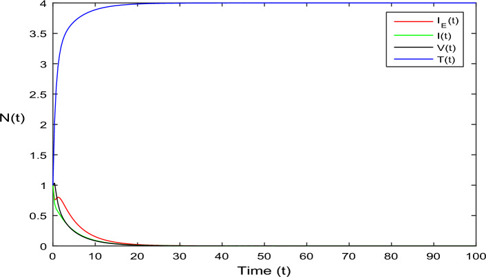
Figure 1.
Dynamics of deterministic HIV model (1) that is .
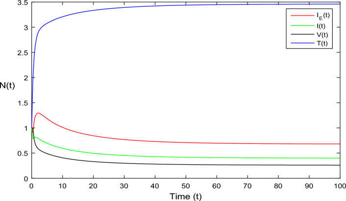
Figure 2.
Dynamics of deterministic HIV model (1) that is
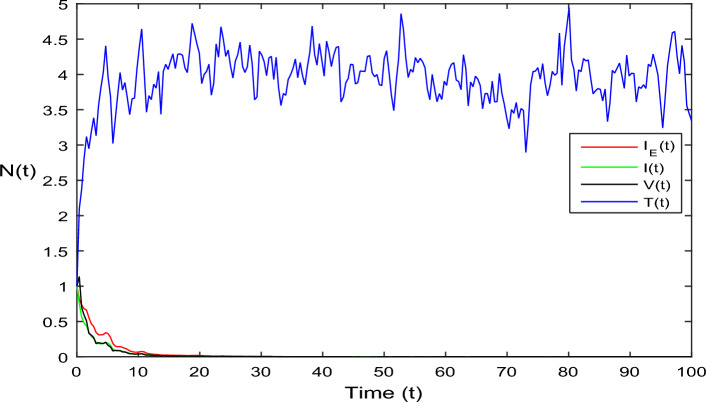
Figure 3.
Dynamics of HIV system Eq. (2) in stochastic case where
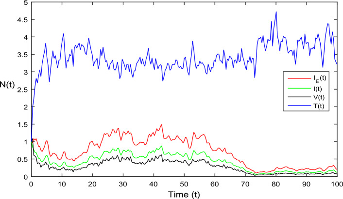
Figure 4.
Simulation of HIV model Eq. (2) in stochastic case where
Figure 5.
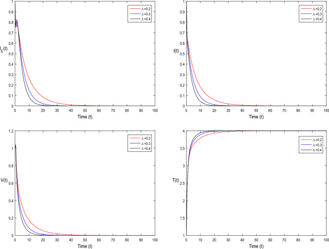
Simulation of deterministic HIV system (1) for different values of , where .
Figure 6.
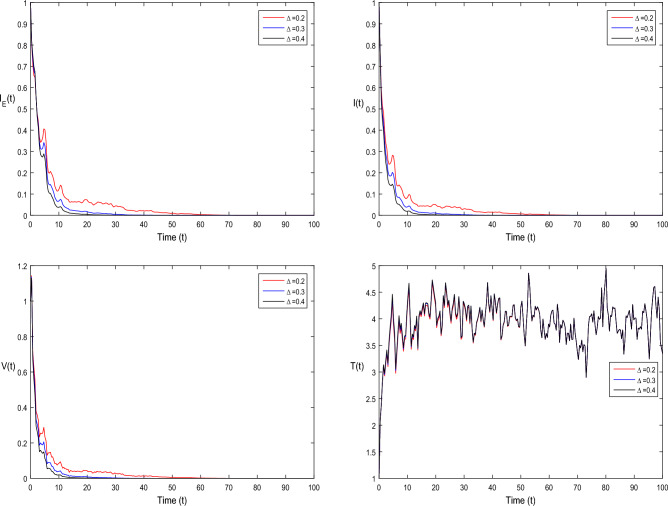
Dynamics of stochastic HIV system (2) for different values of , where .
Figure 7.
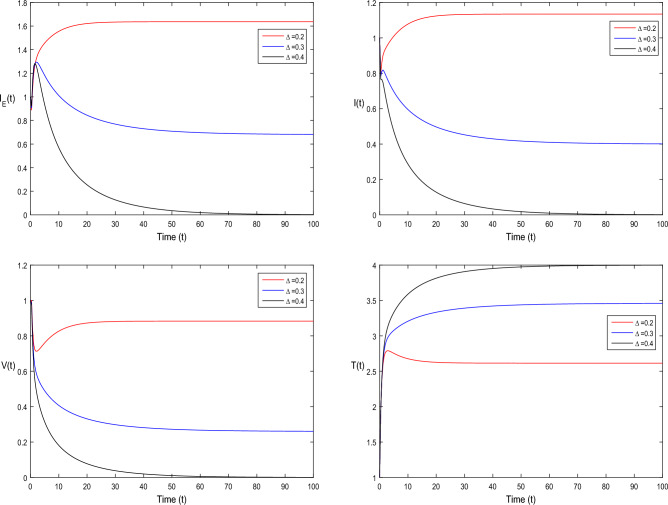
Dynamics of deterministic HIV system (1) for different values of , where .
Figure 8.
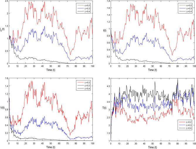
Simulation of stochastic HIV system (2) for different values of , where .
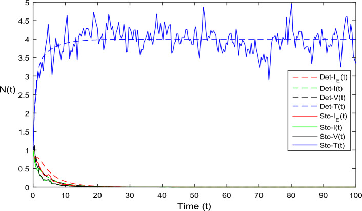
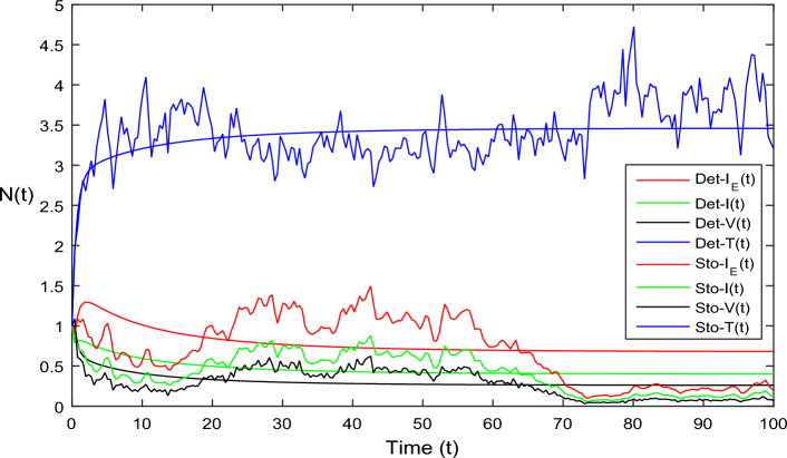
In Fig. 1, the parameter values in Table 1 are assumed for deterministic system Eq. (1). The reproduction number becomes , by using given parameter values. Further, by using Theorem 4.1, we see the model Eq. (1) has a stable infectious-free equilibrium point where is in the form . For Fig. 2, we assume the parameter values given in Table 2, we got , and using theorem 4.1 the model Eq. (1) has a stable endemic equilibrium point as all the compartments are tends to zero as shown in Fig. 2. For Fig. 3, using the Table 1, parameter values for stochastic system Eq. (2). The above simulation shows that and along with theorem 4.5 the infected classes of model Eq. (2) become zero. Likewise, for Fig. 4, employing the parameter values outlined in Table 2, the stochastic model Eq. (2) adhere to , satisfying . Utilizing theorem 4.5, this demonstrates that each class converge to endemic equilibrium as described in equations Eq. (2), which is illustrated in Fig. 4. In Fig. 5, we draw the graphs for different values of delay parameter , using the parameter values of Table 1, for the system Eq. (1). We clearly see that, if we increase the value of , then classes becomes decreases, correspondingly T(t) class become increase. Such dissertation is clearly seen in Fig. 5. Similarly, in Fig. 6 using parameter values given in Table 1, for the stochastic system Eq. (2). Again we see that if we increase the value of , then classes are decreasing, correspondingly T(t) becomes increase. In Fig. 7, we draw the graphs for different values of delay parameter , using the parameter values of Table 2, for the deterministic system Eq. (1). We clearly see that, if we increase the value of , then classes become decreases, correspondingly T(t) class become increase. Such dissertation is clearly seen in Fig. 7. For the above parameter values the proposed system satisfies the endemic equilibrium . Similarly, for Fig. 8, and Table 2, values are assumed for the stochastic system Eq. (2). Again we see that if we increase the value of , then classes are decreasing, consequently T(t) becomes increase. Figure 9 is drawn for the parameter values given in Table 1. For this figure, we show the comparison of the solutions Eqs. (1) and (2). The simple computation shows that for model Eq. (1) , where for stochastic model Eq. (2) with Using the theorems 4.1 and 4.5, we see both the systems satisfy the disease-free equilibriums. Figure 10 is drawn for the Table 2 parameter values. The present figure shows the comparison of the solutions Eqs. (1) and (2). The simple calculations described that the model Eq. (1) have , where for stochastic model Eq. (2) with Again using the Theorems 4.1 and 4.5, we see both the systems satisfy the endemic equilibriums.
Table 1.
Parameter values for .
| Parameters | Values |
|---|---|
| 4 | |
| 0.3 | |
| 1 | |
| 0.3 | |
| 0.8 | |
| 0.9 | |
| C | 1 |
| N | 2 |
| 1 |
Table 2.
Parameter values for .
| Parameters | Values |
|---|---|
| 4 | |
| 0.7 | |
| 1 | |
| 0.3 | |
| 0.9 | |
| 0.8 | |
| C | 1 |
| N | 2 |
| 1 |
Figure 9.
Solution comparison of both HIV systems given in (1) and (2), for
Figure 10.
Solution comparison of both HIV systems given in (1) and (2), for
Conclusion
In conclusion, our research provides a nuanced understanding of the mathematical dynamics of stochastic HIV transmission, considering both time delay and stochasticity. The stability analysis, supported by theorems and lemmas, yields valuable insights into the potential success of control strategies. The findings emphasize the critical importance of timely interventions and sustained efforts in the ongoing global fight against HIV.
We can confidently state that the disease-free equilibrium is proven to be stable asymptotically when becomes less than 1. Conversely, when exceeds 1, the stable endemic equilibrium is established. These results provide significant insights in understanding the dynamics of HIV infection and its potential spread in different population settings. Numerical simulations were performed to examine the influence of the delay parameter () on the proposed models. Various values of were tested, and the impact of this delay was investigated.
As we conclude this research, we call for continued interdisciplinary collaboration between mathematicians, epidemiologists, and public health professionals. The synergy of theoretical insights and empirical data is essential for refining models, validating assumptions, and ultimately informing evidence-based interventions. Our journey in understanding the mathematical intricacies of HIV transmission continues, fueled by the collective commitment to creating a world free from the burden of HIV/AIDS.
In future work, we aim to extend the proposed stochastic HIV model with time delay to corporate the additional complexities such as varying levels of intervention coverage and spatial heterogeneity. Such expansions will allow for a more informative understanding about HIV transmission dynamics across different population subgroups and geographic regions. Furthermore, we extend to integrate real-world data sources to calibrate the model and validate, to enhancing its predictive capabilities for informing evidence based public health strategies.
Acknowledgments
This work was supported by Research Supporting Project Number (RSPD2024R1007), King Saud University, Riyadh, Saudi Arabia. The author Muhammad Bilal Riaz thankful to Ministry of Education, Youth and Sports of the Czech Republic for their support through the e-INFRA CZ (ID:90254). This work is supported by the University Innovation Foundation of China (Grant No. 2022IT101) and the Undergraduate Education Teaching Research and Reform project Foundation of Xinjiang province (Grant No. XJGXZHJG-202213).
Author contributions
S.L. and S.U.K. wrote the original manuscript, and performed theoretical and simulations. S.U reviewed the entire mathematical results and Wrote the manuscript. A.M.M. and N.F.A. performed the computational results, validate all the results with care, project adminstration, and formal analysis. M.B.R. and S.W.T. conceptualized the main problem and perform data analysis, validate all the results with care, restructured the manuscript and funding acquisition. All authors are agreed on the final draft of the submission file.
Data availability
The data that support the findings of this study are available from the corresponding author upon reasonable request. Further, no experiments on humans and/or the use of human tissue samples involved in this study.
Competing interests
The authors declare no competing interests.
Footnotes
Publisher's note
Springer Nature remains neutral with regard to jurisdictional claims in published maps and institutional affiliations.
Contributor Information
Shuo Li, Email: shuoli01001@foxmail.com.
Shewafera Wondimagegnhu Teklu, Email: shewaferaw@dbu.edu.et.
References
- 1.Balaji S, Chakraborty R, Aggarwal S. Neurological complications caused by human immunodeficiency virus (HIV) and associated opportunistic co-infections: a review on their diagnosis and therapeutic insights. CNS Neurol. Disord. Drug Targets (Formerly Curr. Drug Targets-CNS Neurol. Disord.) 2024;23(3):284–305. doi: 10.2174/1871527322666230330083708. [DOI] [PubMed] [Google Scholar]
- 2.Goga, A. et al. The impact of health programmes to prevent vertical transmission of HIV. Advances, emerging health challenges and research priorities for children exposed to or living with HIV: Perspectives from South Africa (2019). [DOI] [PubMed]
- 3.Dieffenbach CW, Fauci AS. Thirty years of HIV and AIDS: Future challenges and opportunities. Ann. Intern. Med. 2011;154(11):766–771. doi: 10.7326/0003-4819-154-11-201106070-00345. [DOI] [PubMed] [Google Scholar]
- 4.Siettos CI, Russo L. Mathematical modeling of infectious disease dynamics. Virulence. 2013;4(4):295–306. doi: 10.4161/viru.24041. [DOI] [PMC free article] [PubMed] [Google Scholar]
- 5.Bentout S, Chekroun A, Kuniya T. Parameter estimation and prediction for coronavirus disease outbreak 2019 (COVID-19) in Algeria. AIMS Public Health. 2020;7(2):306. doi: 10.3934/publichealth.2020026. [DOI] [PMC free article] [PubMed] [Google Scholar]
- 6.Eaton JW, et al. HIV treatment as prevention: Systematic comparison of mathematical models of the potential impact of antiretroviral therapy on HIV incidence in South Africa. PLoS Med. 2012;9(7):e1001245. doi: 10.1371/journal.pmed.1001245. [DOI] [PMC free article] [PubMed] [Google Scholar]
- 7.Ahmed I, et al. Analysis of Caputo fractional-order model for COVID-19 with lockdown. Adv. Differ. Equ. 2020;2020(1):394. doi: 10.1186/s13662-020-02853-0. [DOI] [PMC free article] [PubMed] [Google Scholar]
- 8.Ullah S, et al. The dynamics of HIV/AIDS model with fractal-fractional Caputo derivative. Fractals. 2023;31(02):2340015. doi: 10.1142/S0218348X23400157. [DOI] [Google Scholar]
- 9.Chowell G, et al. Mathematical models to characterize early epidemic growth: A review. Phys. Life Rev. 2016;18:66–97. doi: 10.1016/j.plrev.2016.07.005. [DOI] [PMC free article] [PubMed] [Google Scholar]
- 10.Din A, Sabbar Y, Peng W. A novel stochastic Hepatitis B virus epidemic model with second-order multiplicative a-stable noise and real data. Acta Math. Sci. 2024;44(2):752–788. doi: 10.1007/s10473-024-0220-1. [DOI] [Google Scholar]
- 11.Spencer, S. Stochastic epidemic models for emerging diseases (Doctoral dissertation, University of Nottingham) (2008).
- 12.Anderson RM, et al. Epidemiology, transmission dynamics and control of SARS: The 2002–2003 epidemic. Philos. Trans. R. Soc. Lond. Ser. B Biol. Sci. 2004;359(1447):1091–1105. doi: 10.1098/rstb.2004.1490. [DOI] [PMC free article] [PubMed] [Google Scholar]
- 13.Banks HT, Bortz DM, Holte SE. Incorporation of variability into the modeling of viral delays in HIV infection dynamics. Math. Biosci. 2003;183(1):63–91. doi: 10.1016/S0025-5564(02)00218-3. [DOI] [PubMed] [Google Scholar]
- 14.Madhav, N., Oppenheim, B., Gallivan, M., Mulembakani, P., Rubin, E., & Wolfe, N. Pandemics: risks, impacts, and mitigation. (2018). [PubMed]
- 15.Aral SO, Padian NS, Holmes KK. Advances in multilevel approaches to understanding the epidemiology and prevention of sexually transmitted infections and HIV: An overview. J. Infect. Dis. 2005;191(1):Supplement-1–S6. doi: 10.1086/425290. [DOI] [PubMed] [Google Scholar]
- 16.Heesterbeek H, Anderson RM, Andreasen V, Bansal S, De Angelis D, Dye C, Eames KT, Edmunds WJ, Frost SD, Funk S, Hollingsworth TD, Isaac Newton Institute IDD Collaboration Modeling infectious disease dynamics in the complex landscape of global health. Science. 2015;347(6227):aaa4339. doi: 10.1126/science.aaa4339. [DOI] [PMC free article] [PubMed] [Google Scholar]
- 17.Hébert-Dufresne L, Althouse BM, Scarpino SV, Allard A. Beyond R 0: Heterogeneity in secondary infections and probabilistic epidemic forecasting. J. R. Soc. Interface. 2020;17(172):20200393. doi: 10.1098/rsif.2020.0393. [DOI] [PMC free article] [PubMed] [Google Scholar]
- 18.Mode CJ, Sleeman CK. Stochastic Processes in Epidemiology: HIV/AIDS, Other Infectious Diseases and Computers. World Scientific; 2000. [Google Scholar]
- 19.Gul N, et al. Transmission dynamic of stochastic hepatitis C model by spectral collocation method. Comput. Methods Biomech. Biomed. Eng. 2022;25(5):578–592. doi: 10.1080/10255842.2021.1970143. [DOI] [PubMed] [Google Scholar]
- 20.Ali A, et al. On dynamics of stochastic avian influenza model with asymptomatic carrier using spectral method. Math. Methods Appl. Sci. 2022;45(13):8230–8246. doi: 10.1002/mma.8183. [DOI] [Google Scholar]
- 21.Khan SU, Ali I. Application of Legendre spectral-collocation method to delay differential and stochastic delay differential equation. AIP Adv. 2018;8(3):035301. doi: 10.1063/1.5016680. [DOI] [Google Scholar]
- 22.Khan SU, Ali M, Ali I. A spectral collocation method for stochastic Volterra integro-differential equations and its error analysis. J. Adv. Differ. Equ. 2019;1:161. doi: 10.1186/s13662-019-2096-2. [DOI] [Google Scholar]
- 23.Soufiane B, Touaoula TM. Global analysis of an infection age model with a class of nonlinear incidence rates. J. Math. Anal. Appl. 2016;434(2):1211–1239. doi: 10.1016/j.jmaa.2015.09.066. [DOI] [Google Scholar]
- 24.Baba IA, Yusuf A, Nisar KS, Abdel-Aty AH, Nofal TA. Mathematical model to assess the imposition of lockdown during COVID-19 pandemic. Results Phys. 2021;20:103716. doi: 10.1016/j.rinp.2020.103716. [DOI] [PMC free article] [PubMed] [Google Scholar]
- 25.Baba IA, Rihan FA. A fractional-order model with different strains of COVID-19. Phys. A Stat. Mech. Appl. 2022;603:127813. doi: 10.1016/j.physa.2022.127813. [DOI] [PMC free article] [PubMed] [Google Scholar]
- 26.Ibrahim A, et al. Modeling the dynamics of COVID-19 with real data from Thailand. Sci. Rep. 2023;13(1):13082. doi: 10.1038/s41598-023-39798-9. [DOI] [PMC free article] [PubMed] [Google Scholar]
- 27.Beauchemin CAA, Handel A. A review of mathematical models of influenza A infections within a host or cell culture: Lessons learned and challenges ahead. BMC Public Health. 2011;11(1):1–15. doi: 10.1186/1471-2458-11-S1-S7. [DOI] [PMC free article] [PubMed] [Google Scholar]
- 28.Mahroug F, Bentout S. Dynamics of a diffusion dispersal viral epidemic model with age infection in a spatially heterogeneous environment with general nonlinear function. Math. Methods Appl. Sci. 2023;46(14):14983–15010. doi: 10.1002/mma.9357. [DOI] [Google Scholar]
- 29.Perelson AS. Modelling viral and immune system dynamics. Nat. Rev. Immunol. 2002;2:28. doi: 10.1038/nri700. [DOI] [PubMed] [Google Scholar]
- 30.Hethcote HW. The mathematics of infectious diseases. SIAM Rev. 2000;42:599–653. doi: 10.1137/S0036144500371907. [DOI] [Google Scholar]
- 31.Baltes A, Akpinar F, Inankur B, Yin J. Inhibition of infection spread by co-transmitted defective interfering particles. PLoS ONE. 2017;12:e0184029. doi: 10.1371/journal.pone.0184029. [DOI] [PMC free article] [PubMed] [Google Scholar]
- 32.Liao LE, Iwami S, Beauchemin CA. (In) validating experimentally derived knowledge about influenza A defective interfering particles. J. R. Soc. Interface. 2016;13:20160412. doi: 10.1098/rsif.2016.0412. [DOI] [PMC free article] [PubMed] [Google Scholar]
- 33.Ho DD, Neumann AU, Perelson AS, Chen W, Leonard JM, Markowitz M. Rapid turnover of plasma virions and CD4 lymphocytes in HIV-1 infection. Nature. 1995;373:123. doi: 10.1038/373123a0. [DOI] [PubMed] [Google Scholar]
- 34.Platt EJ, Kozak SL, Durnin JP, Hope TJ, Kabat D. Rapid dissociation of HIV-1 from cultured cells severely limits infectivity assays, causes the inactivation ascribed to entry inhibitors, and masks the inherently high level of infectivity of virions. J. Virol. 2010;84:3106–3110. doi: 10.1128/JVI.01958-09. [DOI] [PMC free article] [PubMed] [Google Scholar]
- 35.Arenas AJ, González-Parra G, Naranjo JJ, Cogollo M, De La Espriella N. Mathematical analysis and numerical solution of a model of HIV with a discrete time delay. Mathematics. 2021;9(3):257. doi: 10.3390/math9030257. [DOI] [Google Scholar]
- 36.Khan, S. U. & Ali, I. Numerical analysis of stochastic SIR model by Legendre spectral collocation method. In Advances in Mechanical Engineering, vol. 11, 7, (SAGE Publications, 2019).
- 37.Ali I, Khan SU. Analysis of stochastic delayed SIRS model with exponential birth and saturated incidence rate. Chaos Solitons Fract. 2020;138:110008. doi: 10.1016/j.chaos.2020.110008. [DOI] [Google Scholar]
- 38.Khan SU, Ali I. Convergence and error analysis of a spectral collocation method for solving system of nonlinear Fredholm integral equations of second kind. Comput. Appl. Math. 2019;38(3):125. doi: 10.1007/s40314-019-0897-2. [DOI] [Google Scholar]
- 39.Khan SU, Ali I. Applications of Legendre spectral collocation method for solving system of time delay differential equations. Adv. Mech. Eng. 2020;12(6):1687814020922113. doi: 10.1177/1687814020922113. [DOI] [Google Scholar]
- 40.Algehyne EA, Khan FU, Khan SU, Jamshed W, Tag El Din ESM. Dynamics of stochastic zika virus with treatment class in human population via spectral method. Symmetry. 2022;14(10):2137. doi: 10.3390/sym14102137. [DOI] [Google Scholar]
- 41.Ali I, Khan SU. A dynamic competition analysis of stochastic fractional differential equation arising in finance via pseudospectral method. Mathematics. 2023;11(6):1328. doi: 10.3390/math11061328. [DOI] [Google Scholar]
- 42.Song, Y. et al.Advances in Difference Eqnarrays2018, 293 (2018).
Associated Data
This section collects any data citations, data availability statements, or supplementary materials included in this article.
Data Availability Statement
The data that support the findings of this study are available from the corresponding author upon reasonable request. Further, no experiments on humans and/or the use of human tissue samples involved in this study.


