Topology Regulated Background Extraction (TRBE) method for eye fundus images

Abstract

One of the initial steps in the preprocessing of digital fundoscopy images is the identification of pixels containing relevant information. This can be achieved through different approaches, one of them is implementing background extraction, reducing the set of pixels to be analyzed later in the process. In this work, we present a background extraction method for digital fundoscopy images based on computational topology. By interpreting binarized images as cubical complexes and extracting their homological groups in 1 and 2 dimensions we identify a subset of luminescence values that can be used to binarize the original grayscale image, obtaining a mask to achieve background extraction. This method is robust to noise and suboptimal image quality, facilitating the analytical pipeline in the context of computer aided diagnosis approaches. This method facilitates the segmentation of the background of a digital fundoscopy image, which allows further methods to focus on pixels with relevant information (eye fundus). This tool is best suited to be implemented in the preprocessing stages of the analytical pipeline by computational ophthalmology specialists.

• •It is robust to noise and low-quality images.
• •Output provides an ideal scenario for down-the-line analysis by facilitating only relevant pixels in a digital fundoscopy.

Graphical abstract

Specifications Table

Subject Area	Computer Science
More specific subject area	Digital Fundoscopy
Method name	Topology Regulated Background Extraction for Digital Fundoscopy (TRBE)
Name and reference of original method	Not applicable.
Resource availability	Not applicable.

Background

Background segmentation in eye fundus images is a critical step in computational ophthalmology, enabling automated analysis for the detection and monitoring of various eye diseases such as diabetic retinopathy, glaucoma, and age-related macular degeneration. The goal of background segmentation is to isolate the anatomical structures of interest (the optic disc, blood vessels, and macula) from the rest of the image to facilitate their detailed examination. This process involves distinguishing these structures from the image background, which may include less relevant anatomical features and noise [9].

Background segmentation in digital eye fundus images presents several significant challenges that complicate the accurate analysis and diagnosis of ocular conditions. One primary issue is the variability in image quality, which can arise from differences in imaging equipment, variations in lighting conditions, and patient-specific factors such as involuntary eye movements or the presence of cataracts, all of which can obscure or distort the anatomical structures of interest. Additionally, the inherent anatomical variation among individuals, such as differences in the size, shape, and color of the optic disc, blood vessels, and macula, poses a considerable challenge, as segmentation algorithms must be robust enough to accurately identify these structures across diverse populations. Pathological conditions further exacerbate these challenges; diseases like diabetic retinopathy, glaucoma, and age-related macular degeneration can significantly alter the appearance of retinal features, necessitating segmentation methods that are adaptable to a wide range of normal and pathological states. Furthermore, the presence of artifacts, such as reflections or shadows, and the need for high precision in distinguishing closely situated or overlapping structures, add layers of complexity to developing effective and reliable background segmentation techniques [2]. Addressing these challenges requires sophisticated image processing and machine learning approaches, capable of accommodating the wide variability and complexity of fundus images.

In computational ophthalmology, the accurate segmentation of eye fundus images is foundational for automated disease detection and monitoring systems [5].

Method details

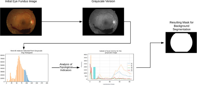
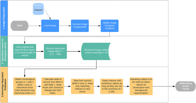
A color eye fundus image is required as input for this method, the process can be summarized in three general phases:

• 1.Image preparation.

  Where the image is loaded, converted into grayscale and the image histogram is obtained.

• 2.Operations based on the image histogram vector.

  Where a subset of luminescence values is selected from the histogram and used as threshold for binarizing the grayscale image, saving the resulting images in a new stack.

• 3.Homology regulated evaluation.

  Where the homological groups in 1 and 2 dimensions are obtained from the set of binarized images generated in the previous steps. Then both vectors (Betti 1 and Betti 2) are analyzed to find the indexes where minimum change in their values is found, these values will be saved as a subset and reported as suitable binarizing threshold values.

The output of the process is a set of integer numbers representing an interval of luminescence values suitable for binarizing the input grayscale image and obtaining a mask for background and foreground segmentation of the eye fundus digital image.

Fig. 1 provides a visual summary of this process:

Fig. 1.

Visual summary of the general process for topology regulated background extraction of eye fundus digital images.

For the examples of the method we will use an image from the APTOS dataset (“ [1] Blindness Detection,” n.d.).

Steps in the algorithm

• 1.
  Load image.

  • •
    Digital fundoscopy images are generally color images, the file is loaded in RGB format using the openCV python package.

    Fig. 2.

    

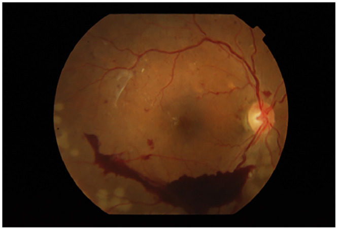    Fundoscopy image from the APTOS dataset (fcc6aa6755e6.png).

• 2.
  Convert color image to grayscale.

  • •
    The conversion is done by the python package openCV following a weighted method using the following formula:
    L= (0.299*R) + (0.587*G) + (0.114*B)

  Where:

  L= luminescence.

  R = red image matrix.

  G = green image matrix.

  B = blue image matrix.

• 3.
  Obtain image histogram.

  • •
    The histogram is obtained by following the formula as presented by (Marques, Oge, 2011) [6]:
    h(k) = n_k = card{(x,y) | f(x,y) = k}
  Where:

  • •
    k= {0,1,…,L - 1}, where L is the number of gray levels in the image.
  • •
    card{...} refers to the cardinality of the set or the number of elements in each set nk.

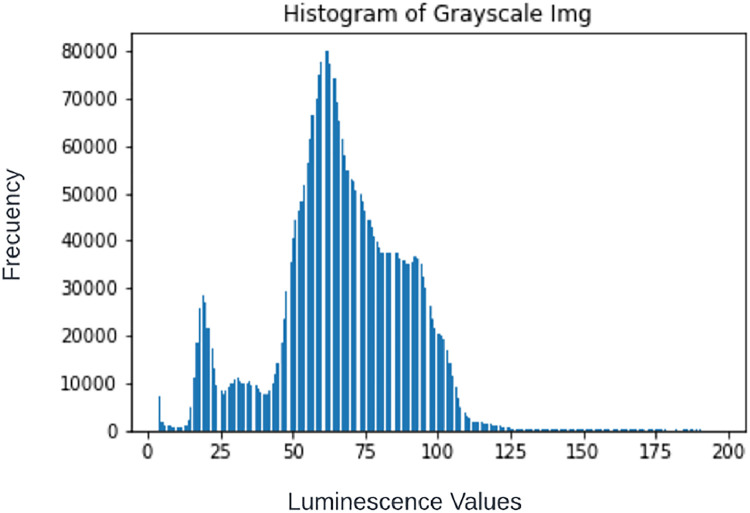
    Fig. 4.

    

    Image histogram obtained from Fig. 3. Notice that indexes 0 through 3 have been omitted since the counter in each of those is very high, given the large number of dark pixels in the image, this only for visualization purposes.

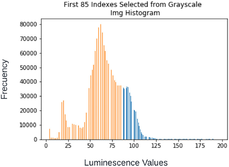
• 4.Once an image histogram is obtained, the values in the first 85 (one third) indexes are selected, this because the goal of the process is to achieve segmentation of the background and, in digital fundoscopy images, pixels representing the background are generally assigned close-to-zero values (dark or complete dark) (Fig. 5).
• 5.
  Binarization of grayscale image using as threshold (t) the first 85 values of luminescence as selected in previous step.

  • •
    Algorithm 1 is used to generate the binarized images.
  • •
    Notice that from each grayscale image, 85 binarized images are obtained.
  • •
    Images are saved in .bmp format.
• 6.
  Obtain homological groups in 1 and 2 dimensions of the binarized images.

  • •
    In order to achieve this the binarized image is saved as a bit map format, then it is interpreted as a cubical complex, for a detailed explanation on cubical complexes and homology see [4].

    • ◦
      A cubical complex K is a collection of cubes that satisfies the following conditions:

      • ■
        Closed under Faces: If a cube is in $\mathrm{K}$, then all of its faces (of all dimensions) are also in $\mathrm{K}$. A face of a cube is any result of selecting a subset of the dimensions of the cube and collapsing the cube along those dimensions to zero length. As an example, the faces of a $3-$dimensional cube include its $2-$dimensional faces (squares), its $1-$dimensional edges, and its $0-$dimensional vertices.
      • ■
        Intersecting Cubes: If two cubes in $\mathrm{K}$ intersect, their intersection is a face of both cubes. This ensures that the intersection of any two cubes in the complex is a lower-dimensional cube that is also part of the complex, maintaining the integrity of the structure corresponding to the space.
      • ■
        Dimension: A cubical complex is said to be of dimension $\mathrm{n}$ if the highest-dimensional cube in $\mathrm{K}$ is n-dimensional. However, a complex can contain cubes of various dimensions, from $0-$dimensional points up to n-dimensional cubes.
    • ◦
      A cube or $n$-cube can be formally defined as the Cartesian product of $n$ intervals of the form $\left[0,1\right]$or a point (in the case of a $0-$dimensional cube).
    • ◦
      More formally, an $\mathrm{n}$-dimensional cube $\mathrm{C}$ can be defined as:

      $$\begin{array}{c}\hfill \mathrm{C}={\mathrm{I}}_1\times {\mathrm{I}}_2\times \dots \times {\mathrm{I}}_{\mathrm{n}},\end{array}$$

      where each ${\mathrm{I}}_{\mathrm{i}}$ is the interval $\left[0,1\right]$ or a degenerate interval $\left\{0\right\}$ or $\left\{1\right\}$, corresponding to the faces of the cube.
    • ◦
      Cubical complexes provide a flexible framework for modeling and analyzing topological spaces, particularly those that naturally conform to a grid-like structure which is the case for an image matrix.
  • •
    Once the image matrix is interpreted as a cubical complex the corresponding homological groups in 0 and1 dimensions are obtained and expressed in Betti 0 (β₀) and 1 (β₁) numbers, for a detailed explanation on cubical complexes and homology see [8].

    • ◦
      In summary, the process of obtaining homological groups involves breaking down the cubical complex into its constituent geometric elements, combining these elements to form chains, identifying which of these chains loop back on themselves to form cycles, and finally distinguishing those cycles that bound higher-dimensional structures to compute the homology groups. For the case of a 2-dimensional cubical complex we have:

      • ■
        $0_{\text{th}}$ Homology Group (${\mathrm{H}}_0$): Reflects the connected components of the complex.
      • ■
        $1_{\text{st}}$ Homology Grupo (${\mathrm{H}}_1$): Reflects loops or edges that do not bound a Surface within the complex.
    • ◦
      Betti numbers are mathematically defined as the rank of the $n-$th homology group ($H_n$) associated with a space. Formally, for a given homology group $H_n$ the $n-$th Betti number $b_n$ is given by: $b_n=rank\left(H_n\right)$. This means that each Betti number summarizes the dimension of its corresponding homology group. In practical terms, when computing the homology groups ($H_0,H_1,H_2,·\dots$) from a cubical or simplicial complex, the Betti numbers will indicate how many independent cycles, holes, voids or components exist a teach level of dimensionality that are not boundaries of higher-dimensional features (Fig. 6).
  • •
    To obtain Betti numbers in both dimensions we use the software Giotto-TDA by the group at EPFL [8], Fig. 7 shows the results of an exercise performed with three binarized images at different threshold values ($t$).
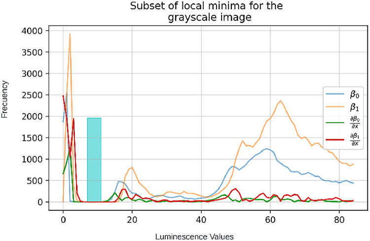
• 7.
  Calculate the rate of change (Δ) among the integers of vectors with β₀ and β₁ numbers and keep the subset of continuous indexes where Δ is minimum per vector.

  • •
    This was done using the NumPy library in Python, specifically the function NumPy.gradient.
  • •
    For this implementation, minimum Δ was considered any value less than 10. The results can be seen in the following vectors:
    Indexes in vector of β₀: [5, 6, 7, 8, 9, 10, 11, 12, 37, 38, 79, 80]
    Indexes in vector of β₁: [7, 8, 9, 10, 11, 12, 13, 14, 15]
• 8.Take the resulting vectors from the two subsets in the previous step (β₀ and β₁) and compare the indexes recorded in both, keep only matching indexes in a new vector named t.

  t = [7, 8, 9, 10, 11]

• 9.
  Keep indexes with discrete values in t if and only if the minimum-plus-one and maximum values (1,85) are not contained in the series.

  • •
    This step is done to assure the mask will not generate values for t near complete dark or too close to the luminescence values where there might be information.

  Notice that the cyan bar represents the interval of continuous indexes that are proposed for the subset t. This maximizes efficacy of the method to produce suitable threshold values for masks for background/foreground extraction.

• 10.The resulting vector t will contain a subset of indexes suitable for binarizing the grayscale version of the input image, obtaining masks that will allow to achieve background and foreground segmentation of the eye fundus image.

Fig. 5.

First third of indexes in image histogram selected from Fig. 4.

Algorithm 1.

Generic image binarization algorithm.

Fig. 6.

Binarized images resulting when applying Algorithm 1 to Fig. 3 using different values for t within the selected indexes in step 4.

Fig. 7.

Examples of calculation of β₀ and β₁ numbers at three different threshold values (t).

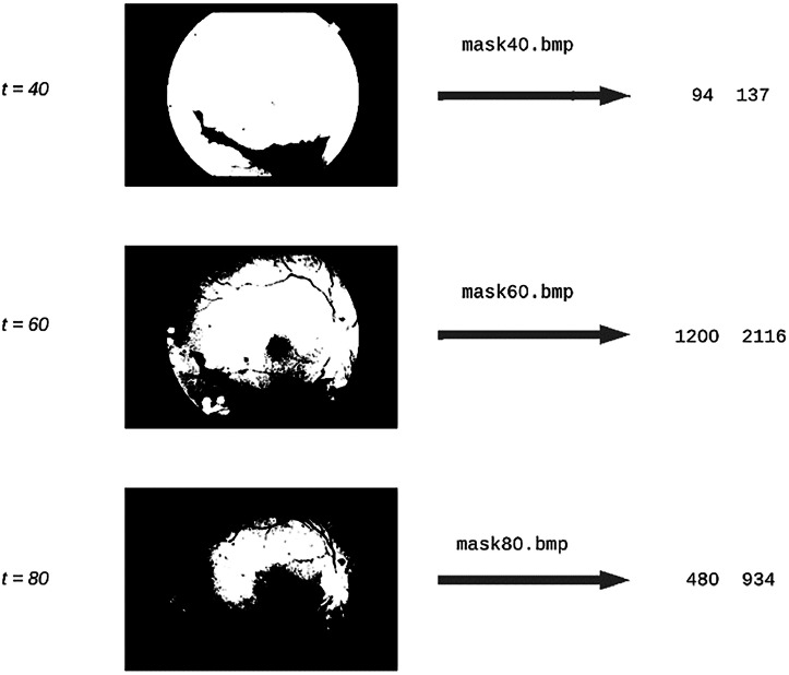
As seen in Fig. 8, all resulting masks are suitable to perform background and foreground extraction in the image shown in Fig. 3. This method is particularly robust to noise and low quality in eye fundus images (Fig. 9).

Fig. 8.

β₀ and β₁ values as well as their Δ, the cyan bar shows indexes where continuous minimum change was detected in both vectors.

Fig. 3.

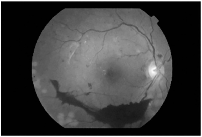
Grayscale version of Fig. 2, converted following the formula shown.

Fig. 9.

Resulting masks applying t values proposed by TRBE.

Method validation

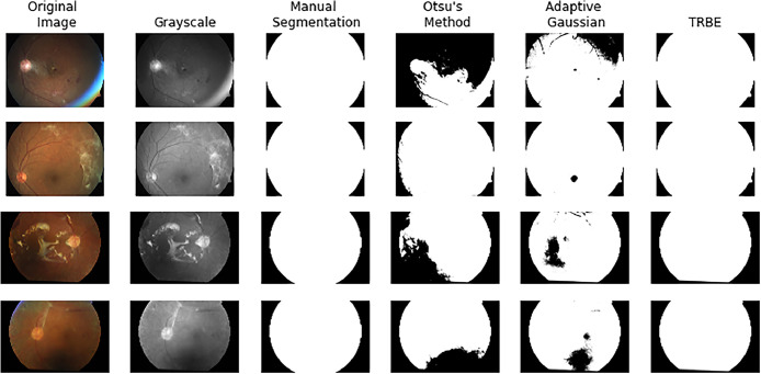
In order to provide information on the performance of the algorithm, a visualization comparing a background segmentation of four noisy images taken from the APTOS dataset performed by two different traditional methods versus TRBE is presented in Fig. 10. As context the color and grayscale versions of the image are presented as well as a manual segmentation of the background performed by the authors for the purpose of applying metric evaluations.

Fig. 10.

Visualization of performance of Otsu´s and Adaptive Gaussian methods versus TRBE for background segmentation. A subset of 4 color image from the APTOS dataset, the corresponding grayscale version and a manual segmentation performned by the authors on the grayscale are added as reference.

The first thresholding approached used is Otsu´s method, which is a global thresholding technique used in image processing. It determines the optimal threshold value for converting a grayscale image into a binary image, effectively separating the foreground from the background. The method assumes that the image contains two classes of pixels (foreground and background) and calculates the threshold that minimizes the intra-class variance or, equivalently, maximizes the inter-class variance. Otsu's method is particularly effective when the histogram of the image has a bimodal distribution, indicating a clear separation between the pixel intensities of the object and the background [7].

The second method evaluated was Adaptive Gaussian thresholding which is a local thresholding technique, meaning that the threshold value is determined for each pixel based on the pixel values in its neighborhood. This method differs from global thresholding techniques like Otsu's method, which use a single threshold value for the entire image. Adaptive Gaussian thresholding calculates the threshold for a pixel by considering a small region around it and applying a Gaussian weighted sum to that region. This approach is particularly useful for images with varying lighting conditions across different areas, as it can adapt the threshold value locally to accommodate these changes. Adaptive Gaussian thresholding helps to preserve detail in regions with significant lighting variation, making it suitable for more complex segmentation tasks where global thresholding methods might fail [3].

In summary, Otsu's method is a global thresholding technique best suited for images with clear bimodal intensity distributions, while Adaptive Gaussian thresholding is a local technique that adjusts the threshold value for each pixel based on its local neighborhood, making it better for images with varying lighting conditions.

The same exercise was performed in 100 randomly selected images from the APTOS dataset, the results obtained are summarised using the following metrics: Mean Square Error (MSE), Structural Similarity Index Measure (SSIM), Mean and Standard Deviation (SD) of Betti numbers in 0-dimension (B0) and 1-dimension (B1) structures. The results are shown in Table 1.

Table 1.

Metric evaluation of background segmentation performance by methods shown in Fig. 10, the median value of MSE and SSIM per image are presented as standard metrics and mean and medians of Betti numbers in zero and one dimension are used to complement the analysis.

Method	MSE Medians	SSIM Medians	B0 Means	B0 SD	B1 Means	B1 SD
Otsu	0.00714	0.99927	698	1608.44	1006	2513.8
Gaussean	0.00714	0.99998	737	1843.82	853	2921.6
TRBE	0.00602	0.99996	3	24.82	6	59.29

The trend observed in Fig. 10 where TRBE is able to perform a more robust background segmentation, particularly in noisy or low quality images can be observed in Table 1 as well, where this same method is able to achieve background segmentation with the least amount of Betti numbers in both dimensions evaluated, which means that it was able to consistently generate segmentation masks with the least of noise caused by connected structures (isolated dots) or holes (incomplete segmented regions).

Limitations

The main limitation we find for this method is when attempting to segment very noisy and severely under illuminated images, this causes the topological method not to be able to successfully perform steps 7,8 and 9 as described in the Method details section. This renders the method unable to find a region of minimum change as indicated in the cyan bar in Fig. 8. Nevertheless, these type of images tend to be rejected for clinical use, given their lack of quality.

Ethics statements

This article does not contain any studies with human or animal participants.

CRediT authorship contribution statement

G.J. Avilés-Rodríguez: Conceptualization, Methodology, Investigation, Software, Writing – original draft. J.I. Nieto-Hipólito: Supervision, Writing – review & editing. M.A. Cosío-León: Supervision, Writing – review & editing. G.S. Romo-Cárdenas: Writing – review & editing. J.D. Sánchez-López: Writing – review & editing. M. Vázquez-Briseño: Writing – review & editing.

Declaration of competing interest

The authors declare that they have no known competing financial interests or personal relationships that could have appeared to influence the work reported in this paper.

Data availability

• Data will be made available on request.

References

- 1.APTOS 2019 Blindness detection [WWW Document], n.d. URL https://kaggle.com/competitions/aptos2019-blindness-detection (accessed 9.18.23).
- 2.Avilés-Rodríguez G.J., Nieto-Hipólito J.I., Cosío-León M., de los Á., Romo-Cárdenas G.S., Sánchez-López J., de D., Radilla-Chávez P., Vázquez-Briseño M. Topological data analysis for eye fundus image quality assessment. Diagnostics. 2021;11:1322. doi: 10.3390/diagnostics11081322. [DOI] [PMC free article] [PubMed] [Google Scholar]
- 3.Gonzalez R.C., Woods R.E. Pearson; New York, NY: 2018. Digital Image Processing. [Google Scholar]
- 4.Kaczynski T., Mischaikow K., Mrozek M. Springer Science & Business Media; 2006. Computational Homology. [Google Scholar]
- 5.Khalid S., Rashwan H.A., Abdulwahab S., Abdel-Nasser M., Quiroga F.M., Puig D. FGR-Net: interpretable fundus image gradeability classification based on deep reconstruction learning. Expert Syst. Appl. 2024;238 doi: 10.1016/j.eswa.2023.121644. [DOI] [Google Scholar]
- 6.Marques O. 1st ed. John Wiley & Sons; 2011. Practical Image and Video Processing Using MATLAB. [Google Scholar]
- 7.Otsu N. A threshold selection method from gray-level histograms. IEEE Trans. Syst. Man Cybern. 1979;9:62–66. doi: 10.1109/TSMC.1979.4310076. [DOI] [Google Scholar]
- 8.Tauzin G., Lupo U., Tunstall L., Pérez J.B., Caorsi M., Medina-Mardones A.M., Dassatti A., Hess K. giotto-tda: a topological data analysis toolkit for machine learning and data exploration. J. Mach. Learn. Res. 2021;22 39–1. [Google Scholar]
- 9.Trucco E., MacGillivray T., Xu Y. Academic Press; 2019. Computational Retinal Image Analysis: Tools, Applications and Perspectives. [Google Scholar]
Associated Data
This section collects any data citations, data availability statements, or supplementary materials included in this article.
Data Availability Statement