Performance investigation of an active free-piston Stirling engine using artificial neural network and firefly optimization algorithm

Abstract

The aim of this study is to explore the characteristics of an active Free-Piston Stirling Engine (AFPSE) through the use of machine learning methods. Due to the time-intensive nature of extracting simulation results from complex thermal equations, an Artificial Neural Network (ANN) is utilized to expedite the process. To construct a nonlinear model, 5000 samples are extracted from simulation results. Input parameters included in the model are the hot and cold source temperatures, the voltage given to the DC motor, spring stiffness, and the mass of the power piston, while output parameters are the amplitude and frequency of power piston displacement. The proposed ANN model structure comprises two hidden layer with 10 and 20 neurons, respectively, indicating the applicability of the ANN model in estimating significant parameters of AFPSE in a shorter amount of time. The firefly optimization algorithm is utilized to determine the unknown input parameters of ANN and maximize the output power. Results indicate that a maximum output power of 23.07 W can be attained by applying 8.5 V voltage on the DC motor. This study highlights the potential of machine learning techniques to explore the primary features of AFPSE.

Nomenclature

$c_p$

Specific heat

C

Damping Coefficient (N.s.m⁻¹)

$D_h$

Hydraulic diameter (m)

$h_C$

Cold cylinder's convective heat transfer coefficient (W/m² k)

$h_H$

Convective heat transfer coefficient in the hot cylinder (W/m² k)

I

Intensity of the received light

$I_0$

Intensity of the main light source

$I_e$

Equivalent Inertia

$I_L$

Inertia of rod

$I_m$

Inertia of DC motor's armature

$I_R$

Inertia of crank

$K_b$

Back electromotive force constant

$K_T$

Torque constant

$k$

Spring stiffness of power piston (N.m⁻¹)

$L$

Length (m)

$L_1$

Inductance (H)

$M$

Total mass of the power piston, rod, and magnet ($kg$)

m

Mass of the gas in engine (kg)

P

Pressure (pa)

$P_r$

Prandtl Number

$R_e$

Resistance $\left(\Omega \right)$

$R_{em}$

Average Reynolds

r

Ideal gas constant

$S_d$

Cross-sectional area of displacer piston (m²)

$S_p$

Cross-sectional area of power piston (m²)

$S_t$

Piston Stroke (m)

$T_C$

Sink temperature (K)

$T_c$

Gas temperature in compression space (K)

$T_H$

Source temperature (K)

$T_h$

Gas temperature in expansion space (K)

$T_m$

Dc motor torque (N.m)

V

Applied voltage to DC motor

W

Work (J)

$x$

Power position of the piston (m)

$\dot{x}$

Power piston velocity (m.s⁻¹)

$\ddot{x}$

Power piston acceleration (m.s⁻²)

$y$

Displacer piston position (m)

γ

Heat capacity ratio

$\nu$

Kinematic viscosity of working gas (m2s-1)

${\eta }_{reg}$

Efficiency of regenerator

$\Delta$

Difference

$\theta$

Angle of rotation of DC motor (degree)

$\mu$

Gas viscosity (pa.s)

$\omega$

Engine frequency (rad.s⁻¹)

$v_{co}$

Initial volume of compression space (m³)

$v_{ho}$

Initial volume of expansion space (m³)

$\beta$

Received attractiveness

${\beta }_0$

attractiveness of the source

1. Introduction

The Stirling engine is an external combustion engine which was introduced by Robert Stirling. One notable advantage of the Stirling engine is its versatility in utilizing different heat sources, including solar energy [1], biomass, and fossil fuels. Active free-piston Stirling engine (AFPSE) is considered an advanced type of dynamic Stirling engine. Free Piston Stirling Engines (FPSEs) belong to the family of Stirling engines, which operate based on the Stirling thermodynamic cycle comprising compression, heating, expansion, and cooling of a sealed working gas to generate power. FPSEs are characterized by their closed-cycle operation, where the working gas remains enclosed within the engine and is continuously cycled. Typically, an FPSE includes two pistons: the power piston and the displacer. The displacer moves the working gas between the hot and cold regions of the engine, while the power piston generates mechanical work by responding to pressure variations due to gas expansion and contraction. In FPSEs, both the power piston and the displacer move in a linear motion, distinct from the rotary motion in many other engine types. The absence of a mechanical linkage, like a crankshaft, connecting the pistons to external components is a fundamental principle of FPSEs. Instead, the piston motion is solely dictated by pressure differentials in the working gas. To enhance thermal efficiency, Stirling engines, including FPSEs, often incorporate a regenerator. This device stores and releases heat within the engine to reduce energy losses and optimize overall performance. FPSEs require an external combustion chamber and a heat sink to maintain the necessary temperature gradient for the Stirling cycle. FPSEs are renowned for their high thermal efficiency and low emissions, making them an environmentally friendly choice suitable for diverse applications such as power generation and waste heat recovery. They have found use in electricity generation, combined heat and power systems [2], and solar power applications, particularly when reliability and efficiency are paramount.

One of the main advantages of AFPSE is the ability to manually adjust the operating frequency, which allows for better adaptability to varying conditions. Numerous researchers have conducted studies on the design, development, key characteristics, and important parameters of Stirling engines. These investigations aim to optimize engine performance, improve efficiency, and explore potential applications in various fields. Buscemi et al. [3] focused on optimizing the collector aperture area of the solar dish-Stirling engine to increase its diffusion. The study showed that an optimized dish-Stirling system could produce approximately 80 MWhe/year in areas with direct irradiation ranging from 2000 to 25000 kWh/m^2. Carrillo Caballero et al. [4] explored a multi-objective optimization approach for the dish Stirling engine. They used a detailed mathematical model to estimate efficiency and output power. Employing the NSGAII optimization algorithm, they successfully minimized heat loss and maximized power, resulting in substantial reductions in heat loss and impressive efficiency and output power figures of 21% and 11.1 kW, respectively. Wenlian Ye et al. [5] conducted multi-objective optimization for the free-piston Stirling engine. The goal of the optimization process was to concurrently enhance output power, thermal efficiency, and exergy efficiency. Various factors, such as gas pressure, piston frequency, temperatures, link size, and phase angle, were taken into consideration. The outcomes revealed optimal parameters, highlighting the significance of high charge pressure, elevated hot end temperature, optimal operating frequency, suitable cooler length, and a specific phase angle. As a result, the predicted efficiencies reached 136 W for output power, 38% for thermal efficiency, and 62% for exergy efficiency. Mingjiang Ni et al. [6] explored the Improved Simple Analytical Model for predicting heat and power loss in Stirling engines. They considered nitrogen and helium gases at varying flywheel speeds and gas pressures. Results indicated that higher flywheel speeds reduced work and the PV diagram area, while increased mean gas pressure enhanced efficiency and power output. The study achieved peak efficiency and output power at 12.2% and 139 W for nitrogen, and 16.5% and 165 W for helium. Schiessler et al. [7] combined the genetic algorithm with a neural network to find a suitable number of layers and neurons for surgery data. The study achieved an accuracy increase of more than 40% and reduced the network size to 15% by using an optimization algorithm. In a separate study [8], an artificial neural network modeled wind turbine power, utilizing wind direction, wind speed, and yaw angle as inputs, and total power as the output. A genetic algorithm optimized the yaw angle, achieving a maximum total power ratio of 0.96 across various operating conditions. Masoumi et al. [9] used an ANN to approximate the function of a solar asphalt collector, improving data extraction efficiency compared to computational fluid dynamics (CFD) simulations. The ANN model effectively predicted key characteristics under various conditions, achieving thermal efficiency predictions of 45% in August and 35% in November. Furthermore, ANN has found extensive application as an intelligent controller in complex mechatronic devices. Tavakolpour-Saleh et al. [10] created an ANN-based controller for a fluidyne Stirling solar engine. This ANN predicted the optimal DC motor frequency for maximizing power output in varying conditions. Experiments confirmed the feasibility and effectiveness of this ANN controller. For example, under specific conditions (390 K, 294 K, 1.5 m), the ANN predicted an optimal frequency of approximately 0.18 Hz, while experimental results found 2.1 Hz to be optimal. This ANN can be integrated with other control methods, such as Model Predictive Control (MPC). Xiao Wu et al. [11] studied a neural network model for dynamic combustion CO2 process (PCC) performance. Their ANN model had six inputs and one output, predicting key PCC characteristics like response time and dynamic trends. The ANN was integrated into Model Predictive Control (MPC), employing a particle swarm optimization algorithm to identify optimal controller parameters. Tavakolpour-Saleh et al. [12] introduced an AFPSE with a mathematical model that optimized power and efficiency. The best results occurred at a specific DC motor frequency, chamber temperatures, spring stiffness, and piston mass, reaching 7.1W power at 9.2 Hz frequency. In a later project [13], a genetic algorithm optimized heat transfer and damping coefficients for an air-fluid-piston Stirling engine (AFPSE) to improve performance estimation. These coefficients were predicted as nonlinear functions based on DC motor frequency. This approach significantly enhanced simulation accuracy, with maximum estimation errors of 4.4% for gas pressure, 3.7% for power piston movement amplitude, and 2.6% for power piston movement frequency compared to experimental data. Hooshang and colleagues [14] introduced a rapid optimization method tailored for Stirling engines. Utilizing a combination of neural networks and experimental data, the researchers aimed to pinpoint crucial design variables like phase angle, displacer stroke, and working frequency specifically for the ST500 Stirling engine. These variables were optimized using the Multi-Layer Perception (MLP) to maximize the engine's power output and efficiency. Wenlian Ye et al. [15] used an artificial neural network to predict a beta-type free piston Stirling engine's dynamic performance, studying the impact of six input parameters. Spring stiffness and piston mass significantly affected the operating frequency. Post-training, high correlation coefficients (R2) were achieved for both training and testing data. Mean relative errors during training were low: 0.85% for operating frequency, 2.78% for amplitude ratio, and 3.19% for phase angle. This highlights the ANN's strong predictive ability for the engine's dynamic performance. Özgören et al. [16] developed an ANN model for predicting torque and power in a helium-fueled beta-type Stirling engine. They achieved excellent results with 5-11-7-1 and 5-13-7-1 network architectures for torque and power prediction, respectively. After training, both engine performance values showed strong correlations (R2 ≈ 1) for both testing and training data, with minimal RMSE and MEP values (RMSE <0.02% and MEP <3.5%). Toghyani [17] developed an ANN model for estimating the power and torque of the Philips M102C Stirling heat engine, where the initial weights were determined by particle swarm optimization. Ahmadi et al. [18] proposed a feed-forward ANN model to predict the Stirling engine's power, demonstrating the effectiveness of the ANN model.

Analyzing the performance of an AFPSE can be a time-consuming process, as it involves solving highly nonlinear equations for each time step. To expedite the calculations, researchers have explored the use of machine learning techniques such as artificial neural networks (ANNs) and optimization algorithms. The primary goal of this study was to investigate the performance of an AFPSE using these machine learning methods. To do so, five key parameters were selected as input data for the ANN: hot and cold chamber temperatures, spring stiffness, mass, and voltage of the DC motor. The ANN was then trained to predict several output parameters, including the amplitude and frequency of power piston displacement, output power, maximum gas pressure, and amplitude of the power piston. Assessing the precision of the Artificial Neural Network (ANN) model involved gauging its performance through output versus target comparisons and error histogram analysis. Further validation ensued by scrutinizing the forecasted frequency and amplitude of the power piston against experimental data. To maximize output power, the firefly optimization algorithm was employed to ascertain the optimal values for input parameters. The study's findings underscore the efficacy of machine learning algorithms in expeditiously exploring the intricate dynamics of complex systems like AFPSE. By combining ANN and optimization algorithms, researchers can quickly identify optimal operating conditions and design parameters, leading to improved performance and efficiency. Descriprion, advantages and disavantages of diffferent optimization algorithms are presented in Table 1.

Table 1.

Descriprion, advantages and disavantages of diffferent optimization algorithms.

Aspect	Firefly Optimization Algorithm (FOA)	Genetic Algorithm (GA)	Teaching-Learning-Based Optimization (TLBO)
Description	FOA is inspired by the mating behavior of fireflies. It uses the concept of attractiveness to simulate light intensity. Fireflies are attracted to brighter fireflies, and their positions are updated accordingly.	GA is a population-based search algorithm that uses the principles of natural selection, crossover, and mutation to evolve a population of potential solutions.	TLBO is based on a teaching-learning model. It involves two phases: the teacher phase (exploitation) and the learner phase (exploration). Students learn from teachers to improve solutions.
Advantages	•Fast convergence. •Population size independence. •Fewer algorithm-specific parameters. •Effective balance of global and local search. •Inspired by real-world behavior.	•Versatility for various problems. •Parallelizable for faster optimization. •Diverse exploration via crossover and mutation. •Population-based for maintaining diversity.	•Effective population dynamics. •Fewer algorithm-specific parameters. •No need for crossover and mutation. •Adaptability for dynamic problems.
Disadvantages	•-May not perform well for all problem types. •-Sensitive to parameter settings. •Limited scalability for very large populations.	•Requires tuning of various parameters. •Can get stuck in local optima. •Slow convergence for complex problems with high-dimensional search spaces.	•May have limited applicability for certain problem types. •Limited exploration due to lack of crossover and mutation. •Requires careful handling of the teacher-student dynamics.

Section 2 introduces the mathematical model governing mechanical, electrical, and thermal equations. Section 3 covers the firefly algorithm, a powerful optimization algorithm used to find optimal parameters. Section 4 discusses the ANN modeling structure, showing predictive frequency and amplitude of power piston displacement based on various inputs. Section 5 integrates the firefly algorithm with the ANN model of the AFPSE to predict maximum output and determine optimal variables.

2. Mathematical background

The open loop AFPSE is a complex system that comprises several interconnected components, including power and displacer pistons, a DC motor, a slider-crank mechanism, expansion and compression chambers, and a mass-spring system. Fig. 1 illustrates these components and their arrangement within the AFPSE.

Fig. 1.

The active free piston Stirling engine a) The prototype AFPSE b) A schematic overview.

The DC motor is a crucial element in the AFPSE's operation as it drives the displacer piston through a slider-crank mechanism, which converts the motor's rotational motion into reciprocating motion. The slider-crank mechanism, on the other hand, is responsible for converting the rotary motion of the DC motor into the reciprocating motion of the displacer piston. The reciprocating motion of the displacer piston inside the cylinder has a direct impact on the working gas displacement, leading to pressure fluctuations that affect the gas pressure inside the cylinder. Gas pressure is closely related to gas temperature, and accurately estimating temperature is crucial for predicting performance accurately. The pressure fluctuations resulting from gas pressure variations excite a 1-DOF mass-spring-damper system that governs the power piston's dynamics. Fig. 2 and Table 2 represent the open-loop block diagram and mechanical, electrical, and thermal equations governing the AFPSE, respectively [12]. Equations (1), (2), (3), (4), (5), (6), (7), (8) represent the required governing equations for the AFPSE. The simulation considers DC motor voltage, hot and cold temperatures, spring stiffness, and Mass as significant inputs, while the amplitude and frequency of the power piston displacement are considered important output features. As evident from the thermal model, the simulation is highly nonlinear, which makes it challenging to analyze and predict the AFPSE's behavior accurately in the less of the time.

Fig. 2.

Open-loop block diagram of the AFPSE.

Table 2.

Governing equations of AFPSE.

Modeling of DC motor [12]	$$\mathrm{V}-K_b\frac{d\theta }{dt}=\frac{R_e}{K_T}{T}_m+\frac{L_1}{K_T}\frac{d{T}_m}{dt}$$ (1)
Kinematic relation of slider crank [12]	$$y=R_m\left(1-\cos \theta \right)-\beta +L\text{where}\beta =L\sqrt{1-{\left(\frac{R_m}{L}\sin \theta \right)}^2}$$ (2)
Dynamic relations of slider crank [12]	$$\{\begin{array}{c}{T}_m=I_e\mathrm{Ӫ}\\ I_e=I_m+I_R+I_L{\left(\frac{R\cos \theta }{\beta }\right)}^2+m_L\left[{\left(\frac{R\cos \theta }{2}\right)}^2+{\left(R\sin \theta +\frac{\sigma L}{2}\right)}^2\right]+m_D{\left(R\mathit{sin}\theta +\sigma L\right)}^2\\ \sigma =\frac{R^2\sin \theta \cos \theta }{\beta L}\end{array}$$ (3)
Thermal modeling [12]	$$\{\begin{array}{c}2\pi \frac{h_h}{\omega }{s}_{pe}\left(T_H-T_h\right)=\frac{mr{T}_c{T}_h}{T_c-T_h}\left(\mathit{ln}\frac{T_h{v}_{co}+T_c\left(S_d{y}_0+v_{ho}\right)}{T_h\left(S_d{y}_0+v_{co}\right)+T_c{v}_{ho}}+\mathit{ln}\frac{T_h\left(S_d{y}_0+S_p{x}_0+v_{co}\right){+T}_c{v}_{ho}}{T_h\left(S_p{x}_0+v_{co}\right)+T_c\left(S_d{y}_0+v_{ho}\right)}\right)+\Delta m\frac{r}{{\rm Y}-1}\left(T_h-T_c\right)\left(1-{\eta }_{reg}\right)\\ 2\pi \frac{h_c}{\omega }{s}_{de}\left(T_C-T_c\right)=-\frac{mr{T}_c{T}_h}{T_c-T_h}\left(\mathit{ln}\frac{T_h{v}_{co}+T_c\left(S_d{y}_0+v_{ho}\right)}{T_h\left(S_d{y}_0+v_{co}\right)+T_c{v}_{ho}}+\mathit{ln}\frac{T_h\left(S_d{y}_0+v_{co}\right){+T}_c({S_p{x}_0+v}_{ho}}{T_h{v}_{co}+T_c\left(S_d{y}_0+S_p{x}_0+v_{ho}\right)}\right)+W-\Delta m\frac{r}{{\rm Y}-1}\left(T_h-T_c\right)\left(1-{\eta }_{reg}\right)\end{array}$$ (4)
Estimated heat transfer coefficient in hot and cold chamber [13]	$$\begin{array}{c}{h}_h=\frac{0.0090{Re}_m^{1.4892}\mu c_p}{2D_h\mathit{Pr}}\\ h_c=\frac{0.0035{Re}_m^{2.0048}\mu c_p}{2D_h\mathit{Pr}}\end{array}$$ (5)
Pressure equation [12]	$$p\left(x,y\right)=\frac{mr{T}_h{T}_c}{T_h\left(s_d\left(y_0-y\right)+s_{p}x+v_{h0}\right)+T_c\left(s_{d}y+v_{h0}\right)}$$ (6)
Mass spring damper mechanism [12]	$$m\frac{d^{2}x}{{dt}^2}+c\frac{dx}{dt}+kx=\left(p\left(x,y\right)-p_0\right)s_p$$ (7)
Estimated damping coefficient [13]	$$C\left(\omega \right)=0.0618{\omega }^7-1.56{\omega }^6+15.79{\omega }^5-80.23{\omega }^4+207.11{\omega }^3-212.50{\omega }^2-88.24\omega +270.37$$ (8)

This section provides an overview of the mathematical equations governing the AFPSE's key components, including the DC motor, slider-crank mechanism, thermal model, pressure model, and mass-spring system [12]. To expedite the time-intensive model calculations, a neural network model is proposed. The amplitude and frequency of the power piston displacement are used to determine important characteristics such as gas pressure and power output. In section 4, an open-loop block diagram with a fast Fourier transform (FFT) is utilized to calculate these parameters.

3. Firefly optimization algorithm

Optimization algorithms are powerful tools used to minimize or maximize objective functions in various applications [1]. Three commonly used optimization algorithms are the genetic algorithm, firefly optimization algorithm (FOA), and teaching-learning based optimization algorithm. In a previous study, an optimization algorithm was used to minimize the discrepancy between experimental and simulation data, enabling the estimation of two unknown coefficients. Among these algorithms, the firefly optimization algorithm (FOA) stands out as a practical toolbox in the field of artificial intelligence. FOA was proposed by Xin-She Yang and has gained recognition for its effectiveness in solving optimization problems.

The main idea of FOA is based on the attractiveness of fireflies. In nature, if the fireflies produce more light and the distance between fireflies is less, they can attract each other more. In computer science, some artificial populations are created that encompass the main information of unknown parameters. The light source is assumed to be in the form of a point. According to the physics law, the intensity of the pointed light has reverse relation with the square of the distance between two fireflies [19]. Equation (9) computes the intensity of the pointed light as:

$$I=\frac{I_0}{r^2}$$ (9)

where I is the intensity of the received light, $I_0$ is the light intensity of the main source of light and r is the distance between the light source and the firefly.

Firefly's attractiveness is proportional to the light intensity seen by adjacent fireflies. The attractiveness of a firefly can be expressed by equation (10) as [19]:

$$\beta \left(r\right)={\beta }_0{e}^{-\gamma r^M}\approx \frac{{\beta }_0}{1+\gamma r^M}\left(M\ge 1\right)$$ (10)

where β refers to the received attractiveness, β₀ is the maximum attractiveness of the source (attractiveness at $r=0$) and γ is the light absorption coefficient. Equation (11) presents a new position of each firefly [19]:

$$x_n^{new}=x_n^{old}+{\beta }_0{e}^{-\gamma r_{mn}^2}\left(x_m-x_n\right)+\mathrm{\alpha }{\mathrm{\epsilon }}_n$$ (11)

where α is a random number, $\mathrm{\epsilon }$ is a random vector, and r is defined using equation (12):

$$r=\parallel x_m-x_n\parallel$$ (12)

The main steps of this algorithm can be seen as the Pseudo code of the firefly algorithm in Fig. 3.

Fig. 3.

Standard flowchart of firefly algorithm.

In this section, the basic concept of the firefly optimization algorithm is reviewed. The main duty of using an optimization algorithm is to find unknown parameters with the aim of minimizing or maximizing the cost function. In section 5, the firefly algorithm will be used to find the unknown initial condition of working the AFPSE in order to maximize the output power.

4. Artificial neural network modeling and validation

Artificial Neural Networks (ANNs) emerge as a formidable tool in the domain of artificial intelligence, finding widespread application across diverse articles in various fields. Modeled after the intricate structure of neurons in the human brain, ANNs exhibit the capacity to discern relationships between input and output variables without relying on prior knowledge of the underlying mathematical model. This methodology, known for its speed and relative simplicity, is depicted in Fig. 4, illustrating the schematic of a neuron's mathematical model. Equation (13) further elucidates the mathematical interrelation within an individual neuron.

$$\mathrm{Y}=f\left(\sum _{i=1}^n{x}_i\times w_i+b\right)$$ (13)

Fig. 4.

Schematic of an artificial neuron.

Various activation functions are employed in Artificial Neural Networks (ANNs). In this article, the chosen activation function is the hyperbolic tangent sigmoid function, as defined by equation (14):

$$y=\frac{1}{1+\exp \left(-2x\right)}-1$$ (14)

4.1. Artificial neural network structure

Within the ANN algorithm, there are typically three layers, visually depicted in Fig. 5. Each layer comprises multiple neurons. The initial layer is the input layer, positioned at the forefront of the ANN, featuring a predetermined number of neurons, precisely mirroring the input layer's neuron count. The subsequent layer, termed the hidden layer, assumes a pivotal role in processing weights and biases to generate outputs. The determination of the hidden layer's neuron count relies on manual adjustments through trial and error, considering the data complexity. Lastly, the third layer, recognized as the output layer, should ideally house neurons equal to the desired quantity.

Fig. 5.

Artificial neural network structure.

4.2. Training phase

The first step in creating an artificial neural network (ANN) is to prepare the training data. It is important to note that the effectiveness of an ANN depends on the quantity and diversity of the data used for training. If the training data is selected appropriately, the ANN can accurately predict outcomes within the specified ranges. For this particular study, 5000 samples were obtained from Simulink and the input range was determined based on the potential conditions outlined in Table 3.

Table 3.

Input data ranges for ANN.

Parameters	Ranges
Voltage (v)	[4–13]
Hot temperature (Co)	[250–1000]
cold temperature (Co)	[10–40]
Stiffness of spring (N. m−1)	[200–1000]
Mass (kg)	[0.6–1.5]

For the training part of the algorithm 70% of the data is selected randomly. The remaining data is also divided by two. Half is used for validation and the other half is used for the test part. Another critical part is to normalize and scale the data to keep it between −1 and +1.

4.3. Learning algorithm

The performance of the designed ANN is investigated by comparing the difference between the predicted and target output data. Mean Square Error is used here as the objective function. Also Levenberg-Marquardt algorithm (LM) which is a combination of gradient descent and Gauss Newton method is utilized in this study. More details on the learning algorithms can be found in Ref. [19].

4.4. Test phase and evaluation

In this subsection, a feed-forward artificial neural network (ANN) with a structure of 5-10-20-2 (as shown in Fig. 6 is proposed. The ANN model is trained using the Levenberg-Marquardt (LM) learning algorithm available in Matlab software, which enables the determination of the unknown weights and thresholds of the ANN model.The neural network toolbox provided by Matlab is used for training the ANN model. Fig. 7 depicts the training process of the AFPSE ANN model, where the mean square error (MSE) is used as the performance metric. The plot demonstrates the MSE values for the training, validation, and test datasets as the training progresses through epochs. It can be observed from Fig. 7 that the ANN model achieves an acceptable MSE value of approximately 10e-2 after 296 epochs for all three datasets (training, validation, and test). This indicates that the ANN model has successfully learned the patterns and relationships within the AFPSE data and can provide accurate predictions for unseen samples. Table 4 presents information to find the proper ANN model.

Fig. 6.

Proposed artificial neural network modeling for AFPSE.

Fig. 7.

Convergence of MSE for the proposed ANN model of AFPSE.

Table 4.

Detailed information on how to achieve the appropriate ANN model.

Neural network Architechture	MSE	Epoch	Regression analysis of Trainig data		Regression analusis for Validation data		Regression analusis for test data
			Amplitude	frequency	Amplitude	frequency	Amplitude	frequency
5-5-2	0.0043	608	0.9822	0.9998	0.9832	0.9998	0.9845	0.9998
5-10-2	0.001	200	0.9964	0.9998	0.9964	0.9998	0.996	0.9998
5-15-2	0.0006	462	0.9982	0.9998	0.998	0.9998	0.9978	0.9998
5-20-2	0.0008	938	0.9972	0.9998	0.9972	0.9998	0.9971	0.9998
5-25-2	0.0003	586	0.9988	0.9999	0.9987	0.9999	0.9987	0.9999
5-30-2	0.0003	521	0.9989	0.9999	0.9988	0.9999	0.9986	0.9999
5-35-2	0.0004	783	0.9986	0.9999	0.998	0.9999	0.9985	0.9999
5-40-2	0.0002	417	0.9991	0.9999	0.999	0.9999	0.9989	0.9999
5-45-2	0.0003	733	0.9989	0.9999	0.9989	0.9999	0.9987	0.9999
5-50-2	0.0003	354	0.999	0.9999	0.9988	0.9999	0.9988	0.9999
5-55-2	0.0002	714	0.9992	0.9999	0.9989	0.9999	0.9986	0.9999
5-60-2	0.0002	943	0.9993	0.9999	0.999	0.9999	0.9989	0.9999
5-5-5-2	0.0007	999	0.9972	0.9999	0.9976	0.9999	0.9972	0.9998
5-5-10-2	0.0004	817	0.9985	0.9999	0.9984	0.9999	0.9983	0.9999
5-5-15-2	0.0003	670	0.9989	0.9999	0.999	0.9999	0.9989	0.9999
5-5-20-2	0.0002	994	0.9991	0.9999	0.999	0.9999	0.9992	0.9999
5-5-30-2	0.0002	776	0.9995	0.9999	0.9994	0.9999	0.9994	0.9999
5-5-40-2	0.0002	213	0.9995	0.9999	0.9993	0.9999	0.9994	0.9999
5-5-50-2	0.0002	679	0.9995	0.9999	0.9994	0.9999	0.9994	0.9999
5-10-5-2	0.0003	927	0.9988	0.9999	0.9986	0.9999	0.9986	0.9999
5-10-10-2	0.0002	654	0.9992	0.9999	0.9991	0.9999	0.9991	0.9999
5-10-15-2	0.0002	322	0.9993	0.9999	0.9991	0.9999	0.9992	0.9999
5-10-20-2	0.0001	296	0.9995	0.9999	0.9994	0.9999	0.9994	0.9999
5-10-30-2	0.0001	716	0.9996	0.9999	0.9994	0.9999	0.9993	0.9999
5-10-40-2	0.0001	885	0.9996	0.9999	0.9994	0.9999	0.9995	0.9999
5-10-50-2	0.0001	929	0.9996	0.9999	0.9994	0.9999	0.9993	0.9999
5-15-5-2	0.0002	702	0.9992	0.9999	0.999	0.9999	0.9991	0.9999
5-15-10-2	0.0001	813	0.9995	0.9999	0.9993	0.9999	0.9994	0.9999
5-15-15-2	0.0002	533	0.9993	0.9999	0.9992	0.9999	0.9992	0.9999
5-15-20-2	0.0002	971	0.9993	0.9999	0.999	0.9999	0.9992	0.9999
5-15-30-2	0.0001	502	0.9997	0.9999	0.9994	0.9999	0.9994	0.9999
5-15-40-2	0.0001	298	0.9997	0.9999	0.9995	0.9999	0.9994	0.9999
5-15-50-2	0.0001	963	0.9996	0.9999	0.9994	0.9999	0.9995	0.9999
5-20-5-2	0.0002	843	0.9993	0.9999	0.9991	0.9999	0.9991	0.9999
5-20-10-2	0.0001	471	0.9994	0.9999	0.9992	0.9999	0.9992	0.9999
5-20-15-2	0.0001	488	0.9996	0.9999	0.9994	0.9999	0.9994	0.9999
5-20-20-2	0.0001	407	0.9996	0.9999	0.9995	0.9999	0.9995	0.9999
5-20-30-2	0.0001	559	0.9994	0.9999	0.9991	0.9999	0.9992	0.9999
5-20-40-2	0.0001	802	0.9998	0.9999	0.9995	0.9999	0.9994	0.9999
5-20-50-2	0.0001	441	0.9997	0.9999	0.9994	0.9999	0.9994	0.9999

Regression plots serve as tools to anticipate the output parameter. Examining Fig. 8, Fig. 9 reveals the results of regression and error histograms across training, validation, and test data. These visualizations effectively highlight any outliers present in the data. In terms of regression plots, the rank correlations (R) approach 1, indicating a close alignment between the predicted outputs from the ANN model and the actual experimental data. Furthermore, the error distribution, as evidenced by the histograms, displays symmetry, with both the mean error (μ) and standard deviation (σ) nearing 0. This alignment underscores the effective performance of the ANN model across training, validation, and testing datasets.

Fig. 8.

Predicted output vs target and error histograms for the amplitude of the ANN model (a) training data (b) validation data (c) test data.

Fig. 9.

Predicted output vs target and error histograms for power piston frequency of the ANN model (a) training data (b) validation data (c) test data.

4.5. Experiments and model validation

The experimental configuration used to measure power piston displacement and estimate output power at different DC motor frequencies is depicted in Fig. 10. To predict the thermodynamic work and output power of AFPSE, it is crucial to determine the vibration amplitude and frequency of the power piston. This quantity was measured using an ultrasonic sensor with a resolution of 1 mm. In addition, a type K thermocouple was used to measure the temperatures of the hot and cold chambers, and an Arduino Uno collected the data with a sampling period of 0.01 s, satisfying the Nyquist sampling criterion for the engine's maximum frequency.

Fig. 10.

Experimental AFPSE with an ultrasonic sensor to measure amplitude and power piston displacement.

The experiments were done with 450C^o and 245C^o, spring stiffness of 260 N.m-1, a mass of 0.65 kg. and different frequency of DC motor. Then, the maximum amplitude of the power piston motion is measured and compared with the proposed ANN results. The maximum amplitude comparison can be seen in Fig. 11. The results clearly show that the proposed ANN can predict the amplitude of power piston vibration under different DC motor frequencies.

Fig. 11.

Experimental and ANN simulated power piston displacement for different frequencies of DC-motor at T_H = 245C^o and T_H = 450C^o.

In this section, we propose a neural network to predict the amplitude and frequency of power piston displacement. While the mathematical model developed in previous work [13] was accurate, solving the thermal equation was time-consuming. To overcome this challenge, we employ an ANN and use simulation results to train the model. We propose an ANN with a 5-10-20-2 structure and plot regression and error histograms to show the model's performance. Subsequently, we conduct experiments to validate the output of the ANN. In the next section, we will use the proposed ANN model to investigate the main features of AFPSE.

5. Results and discussion

This section employs the proposed ANN model obtained in section 4 to evaluate the performance of an AFPSE. The ANN model takes five inputs, including the voltage applied to the DC motor, hot and cold chamber temperatures, spring stiffness, and power piston mass. Its output is the frequency and amplitude of power piston displacement. The pressure-volume (P–V) plot is an essential figure to investigate Stirling engines. The area enclosed by the P–V curve represents the work done by the engine. To draw the P–V diagram, the sine function is used to simulate the power piston displacement. Equation (15) is used to show the real-time power piston displacement. The time step for estimating the displacement versus time is 0.01.

$$X=Amplitude\times \sin \left(2\pi \times frequency\times time\right)$$ (15)

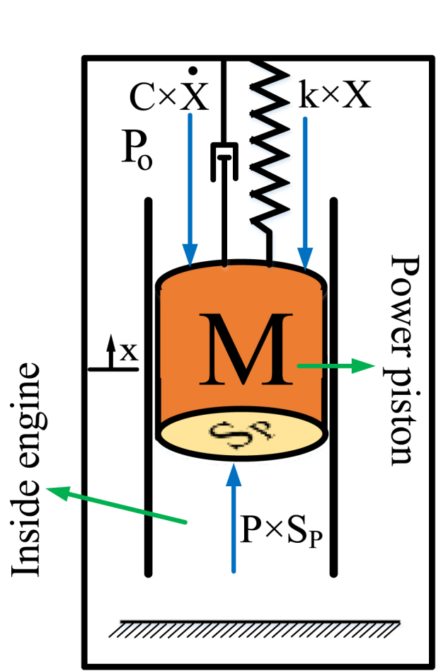
Then, newton^'s second law is used in equation (16) to calculate the gas pressure inside the engine using the power piston displacement, velocity, and acceleration (see Fig. 12).

$$p\left(x\right)=\frac{\left(M\frac{d^{2}x}{{dt}^2}+c\frac{dx}{dt}+kx\right)}{s_p}+p_0$$ (16)

Fig. 12.

Free body diagram of the power piston.

By predicting the power piston displacement and gas pressure, the P–V diagram can be plotted for more investigation. Afterward, the trapezoidal rule is employed to calculate the area of the P–V diagram. The calculated area of the P–V diagram is viewed as the work done by the thermodynamic cycle [20]. The output power of the Stirling engine can be determined by multiplying the work by the frequency of power piston displacement. Equation (17) illustrates the output power relation. Fig. 13 depicts the steps for predicting the P–V diagram, work, gas pressure, and output power of AFPSE.

$$\text{Output}\text{power}=\text{Area}{}_{\mathrm{p}-\mathrm{v}}\times \text{power}\text{piston}\text{frequency}$$ (17)

Fig. 13.

Steps through the calculation of predicting the performance of AFPSE.

In the following, the P–V diagram with different initial conditions is calculated and plotted. Fig. 14 shows the P–V diagram based on the proposed ANN and block diagram. The initial conditions for simulation can be seen in Table 5. The P–V diagrams in four different conditions are plotted in Fig. 14. Table 6 provides information about predicting the work and output power based on the obtained P–V diagram.

Fig. 14.

Predicted P–V diagram of the AFPSE by proposed ANN a) DC motor frequency variable b) hot temperature variable c) mass variable d) stiffness offspring variable.

Table 5.

Initial inputs for investigating the p-v diagram.

Number of Cases	parameters
	Frequency of DC motor (Hz)	TH (Co)	Mass (kg)	Spring stiffness (N.m−1)	TC (Co)
Case (a)	Variable	500 Co	0.8 kg	200 N m−1	10 Co
Case (b)	4.27 Hz	Variable	1.3 kg	300 N m−1	15 Co
Case (c)	4 Hz	800 Co	Variable	400 N m−1	20 Co
Case (d)	3.17 Hz	400 Co	1.5 kg	Variable	13 Co

Table 6.

Predicting the work and output power according to the p-v diagram.

As can be seen in Fig. 14 and Table 6, the P–V diagrams provide information about the performance of AFPSE. In other words, ANN can be used as a nonlinear model to estimate the main feature of the Stirling engine such as optimal frequency, gas pressure, work, and output power in various working conditions in less time. Therefore, more investigations are being done to deeply understand the behavior of AFPSE. Fig. 15, Fig. 16, Fig. 17, Fig. 18 show the maximum amplitude, maximum gas pressure, and output power versus different voltage and frequencies of the DC motor.

Fig. 15.

(a) Maximum amplitude of power piston displacement, (b) gas pressure, and (c) Output power predicted by ANN with M = 1.3 kg, k = 800 N m⁻¹, and, T_C = 20C^o.

Fig. 16.

(a) Maximum amplitude of power piston displacement, (b) gas pressure, and (c) Output power predicted by ANN with T_H = 500C^o K = 250N. m⁻¹ and, T_C = 28C^o.

Fig. 17.

(a) Maximum amplitude of power piston displacement, (b) gas pressure, and (c) Output power predicted by ANN with T_H = 500 C^o, M = 1 kg, and, T_C = 12C^o.

Fig. 18.

(a) Maximum amplitude of power piston displacement, (b) gas pressure, and (c) Output power predicted by ANN with T_H = 700C^o and M = 0.7 kg, and k = 400 N.m⁻¹..

By altering the temperatures of the hot and cold sources, observable trends emerge. Specifically, elevating the hot temperature while concurrently reducing the cold temperature results in an upswing in both the maximum gas pressure and output power. Notably, throughout these temperature variations, the optimal frequency or voltage of the DC remains consistent. Changing the cold temperature has slight effects on the output power. With regard to Fig. 16, Fig. 17, changing the power piston mass and spring stiffness directly influences the optimal voltage of the DC motor. Increasing the power piston mass results in a decrease in the optimal DC motor voltage. The optimal DC motor voltage decreased from 9.6V to 7.5 V, while the power piston mass increased from 0.6 kg to 1.5 kg. Increasing the spring stiffness also leads to an increase in the optimal frequency of the DC motor. Based on Fig. 17, the optimal frequency of the DC motor decreases from 6.1 Hz to 3.9 Hz when the spring stiffness declines from 1000 N m⁻¹ to 200 N m⁻¹.

5.1. Firefly optimization algorithm applied to ANN

In this subsection, the focus is on applying the firefly optimization algorithm to the proposed ANN model of AFPSE with the aim of determining the optimal unknown parameters. Fig. 15, Fig. 16, Fig. 17, Fig. 18 illustrate that AFPSE has the highest output power at a specific frequency of the DC motor based on the initial parameters. Therefore, it is crucial to find the optimal DC frequency and voltage, hot and cold source temperature, mass of the power piston, and spring stiffness. To facilitate this process of finding the optimal parameters, an optimization algorithm is used. The cost function of FOA is set as the output power (see equation (17)), and all input parameters of the ANN model are treated as unknown parameters. FOA is employed to determine the initial condition of AFPSE in order to maximize its output power. To this end, 20 artificial fireflies with 300 iterations are utilized to find the optimal parameters. The block diagram of the firefly optimization algorithm combined with the ANN model of AFPSE is shown in Fig. 19. The convergence plot and the highest cost for the optimization algorithm can also be seen in Fig. 20.

Fig. 19.

Steps through the calculation of finding optimal parameters of AFPSE using the firefly optimization algorithm.

Fig. 20.

Convergence plot and the highest Cost for the firefly optimization algorithm.

As can be seen from, the maximum output power is approximately 23 W and about 150 iterations are required to reach this value. For more investigation, this test was run 10 times and the same result occurred. The optimal value obtained from the firefly optimization algorithm can be seen in Table 7. Furthermore, the optimal P–V diagram is depicted in Fig. 21. The results show that increasing the temperature differences between chambers, power piston mass, and stiffness spring paves the way to reach the maximum output power.

Table 7.

Optimal parameters obtained from the firefly optimization algorithm.

parameters	Optimal value	parameters	Optimal value
TH	1000o	mass	1.5 kg
TC	10Co	Spring stiffness	1000 N m−1
Output power	23.07 W	Frequency of power piston displacement	5.33 Hz
work	4.33 J	The amplitude of power piston displacement	3.4 cm
Maximum pressure	138.89 kPa	The voltage of the DC motor	8.5 V

Fig. 21.

Optimal p-v diagram predicted by ANN model and firefly algorithm of AFPSE.

In this section, the proposed ANN model in section 4 was used for the parametric study. First, the P–V diagrams were investigated under different initial conditions. Afterward, the amplitudes of the power piston displacement, maximum gas pressure, work, and output power were investigated. The results clearly showed that changing the mass of the power piston and spring stiffness had a significant influence on the optimal frequency of the DC motor that maximizes the output power. In addition, changing the temperature difference had no impact on the optimal frequency, but increasing it leads to an increase in the output power. In the end, the firefly optimization algorithm was added to the ANN model in order to find the optimal unknown parameters to maximize the output power.

6. Conclusion and recommendation

This study employed a neural network to predict crucial parameters of an AFPSE, including power piston displacement amplitude and frequency, maximum gas pressure, work, optimal DC motor voltage, and output power under varying operational conditions. While a detailed analytical model for the mechatronic system was previously established and demonstrated in Ref. [12], it had limitations such as slow convergence due to solving highly nonlinear thermal equations in each Simulink time step, making it unsuitable for parametric studies. To address this challenge, an Artificial Neural Network (ANN) was introduced as a nonlinear model to expedite predictions. A three-layer feed-forward ANN with a structure of 5-10-20-2 was suggested to learn the power piston displacement characteristics with five variable inputs. Out of various ANN structures, the 5-10-20-2 configuration exhibited the lowest mean square error and the least complexity. Subsequently, the AFPSE's performance was forecasted, and key features such as output power, maximum gas pressure, power piston displacement amplitude and frequency, P–V (Pressure-Volume) diagram, and work were examined in detail. The results clearly demonstrate the feasibility of utilizing the ANN model for efficient performance analysis. Notably, the findings reveal that temperature differences between the hot and cold chambers have a significant impact on output power. An increase in the hot source temperature and a decrease in the cold source temperature result in a substantial rise in output power. For instance, when parameters are set to M = 1.3 kg, k = 300 N.m-1, and Tc = 15 °C, increasing the hot temperature from 200 °C to 1000 °C increases output power from 1.07 W to 6.11 W. Furthermore, it was observed that temperature has a minor influence on the optimal frequency of the DC motor. In other words, changes in temperature differences between sources do not significantly alter the DC motor's optimal frequency. Increasing the mass of the power piston displacement lowers the optimal frequency of the DC motor while boosting output power. Conversely, increasing spring stiffness reduces the optimal frequency.

In the end, the Firefly Optimization Algorithm was integrated with the proposed neural network model for the AFPSE to determine the optimal initial parameters. The optimization algorithm's cost function was defined as the output power, calculated by multiplying the area enclosed by the closed-loop thermodynamic cycle with the frequency of power piston displacement. The unknown parameters included the temperatures of the hot and cold sources, the mass of the power piston, spring stiffness, and the voltage applied to the DC motor. The Firefly Optimization Algorithm was specifically applied to the neural network model of the engine to maximize the output power. To achieve this, FOA was executed with an initial population size of 20 and 300 iterations. Multiple simulations were carried out to ensure the algorithm didn't get stuck in a local extremum. The final outcomes revealed that the optimal parameters led to an output power of 23.42 W, a DC motor frequency of 5.27 Hz, and a maximum gas pressure of 138.27 kPa.

The primary utilization of the suggested AFPSE lies within renewable energy systems for the conversion of energy. Biofuels, biomass, solar energy, geothermal sources are well-suited for supplying heat to the proposed Stirling converter, facilitating electricity generation. Nevertheless, there is an ongoing need for further development to scale up and industrialize this converter. Future research endeavors will focus on enhancing output power by implementing model predictive control for the converter, mitigating engine vibrations, and designing a more efficient linear alternator based on the ANN model.

CRediT authorship contribution statement

A.P. Masoumi: Conceptualization. A.R. Tavakolpour-Saleh: Supervision. V. Bagherian: Conceptualization.

Declaration of competing interest

The authors declare that they have no known competing financial interests or personal relationships that could have appeared to influence the work reported in this paper.

References

- 1.Masoumi A.P., Bagherian V., Tavakolpour-Saleh A.R., Masoomi E. A new two-axis solar tracker based on the online optimization method: Experimental investigation and neural network modeling. Energy and AI. 2023;14:100284. [Google Scholar]
- 2.Bagherian V., Salehi M., Mahzoon M. Rigid multibody dynamic modeling for a semi-submersible wind turbine. Energy Convers. Manag. 2021;244:114399. [Google Scholar]
- 3.Buscemi A., Guarino S., Ciulla G., Lo Brano V. A methodology for optimisation of solar dish-Stirling systems size, based on the local frequency distribution of direct normal irradiance. Appl. Energy. 2021;303 [Google Scholar]
- 4.Caballero G.E.C., et al. Optimization of a Dish Stirling system working with DIR-type receiver using multi-objective techniques. Appl. Energy. 2017;204:271–286. [Google Scholar]
- 5.Ye W., Yang P., Liu Y. Multi-objective thermodynamic optimization of a free piston Stirling engine using response surface methodology. Energy Convers. Manag. 2018;176:147–163. [Google Scholar]
- 6.Ni M., et al. Improved Simple analytical model and experimental study of a 100 W β-type stirling engine. Appl. Energy. 2016;169:768–787. [Google Scholar]
- 7.Schiessler E.J., Aydin R.C., Linka K., Cyron C.J. Neural network surgery: combining training with topology optimization. Neural Network. 2021;144:384–393. doi: 10.1016/j.neunet.2021.08.034. [DOI] [PubMed] [Google Scholar]
- 8.Sun H., Qiu C., Lu L., Gao X., Chen J., Yang H. Wind turbine power modelling and optimization using artificial neural network with wind field experimental data. Appl. Energy. 2020;280 [Google Scholar]
- 9.Masoumi A.P., Tajalli-Ardekani E., Golneshan A.A. Investigation on performance of an asphalt solar collector: CFD analysis, experimental validation and neural network modeling. Sol. Energy. 2020;207:703–719. [Google Scholar]
- 10.Tavakolpour-Saleh A.R., Jokar H. Neural network-based control of an intelligent solar Stirling pump. Energy. 2016;94:508–523. [Google Scholar]
- 11.Wu X., Shen J., Wang M., Lee K.Y. Intelligent predictive control of large-scale solvent-based CO2 capture plant using artificial neural network and particle swarm optimization. Energy. 2020;196 [Google Scholar]
- 12.Tavakolpour-Saleh A.R., Zare S.H., Bahreman H. A novel active free piston Stirling engine: modeling, development, and experiment. Appl. Energy. 2017;199:400–415. [Google Scholar]
- 13.Masoumi A.P., Tavakolpour-Saleh A.R. Experimental assessment of damping and heat transfer coefficients in an active free piston Stirling engine using genetic algorithm. Energy. 2020;195 [Google Scholar]
- 14.Hooshang M., Moghadam R.A., Nia S.A., Masouleh M.T. Optimization of Stirling engine design parameters using neural networks. Renew. Energy. 2015;74:855–866. [Google Scholar]
- 15.Ye W., Wang X., Liu Y. Application of artificial neural network for predicting the dynamic performance of a free piston Stirling engine. Energy. 2020;194 [Google Scholar]
- 16.Özgören Y.Ö., Çetinkaya S., Sarıdemir S., Çiçek A., Kara F. Predictive modeling of performance of a helium charged Stirling engine using an artificial neural network. Energy Convers. Manag. 2013;67:357–368. [Google Scholar]
- 17.Toghyani S., Ahmadi M.H., Kasaeian A., Mohammadi A.H. Artificial neural network, ANN-PSO and ANN-ICA for modelling the Stirling engine. Int. J. Ambient Energy. 2016;37(5):456–468. [Google Scholar]
- 18.Ahmadi M.H., Sorouri Ghare Aghaj S., Nazeri A. Prediction of power in solar stirling heat engine by using neural network based on hybrid genetic algorithm and particle swarm optimization. Neural Comput. Appl. 2013;22(6):1141–1150. [Google Scholar]
- 19.Wang X., Lin X., Dang X. Supervised learning in spiking neural networks: a review of algorithms and evaluations. Neural Network. 2020;125:258–280. doi: 10.1016/j.neunet.2020.02.011. [DOI] [PubMed] [Google Scholar]
- 20.Yousefzadeh H., Tavakolpour-Saleh A.R. A novel unified dynamic-thermodynamic method for estimating damping and predicting performance of kinematic Stirling engines. Energy. 2021;224 [Google Scholar]