

Abstract
In the complex Internet of Things (IoT) environment, a plethora of IoT services with akin functions but varying qualities of service exist. To meet diverse customer needs and drive widespread application, service composition optimization becomes crucial. In the current era of rapid development in artificial intelligence, intelligent algorithms play a significant role in optimizing service composition. However, algorithms applied to IoT service composition optimization face common challenges of low search efficiency and insufficient optimization precision, including the Shuffled Frog Leaping Algorithm (SFLA) and Genetic Algorithm (GA). Therefore, this study seeks to enhance the perception of service quality in IoT service composition. It proposes an improved SFLA (ISFLA) based on the original SFLA. The algorithm integrates chaos theory and reverse learning theory for the acquisition of the initial population. It utilizes Euclidean distance to partition the population into groups and employs Gaussian mutation to optimize the optimal individual of each group. Finally, the entire population undergoes evolution through a local update method based on two strategies. Simulated experiments were conducted to search for optimal IoT service composition solutions of different scales. The results indicate that, compared to the SFLA, GA, ISFLA*, IGSFLA and SFLAGA, ISFLA achieves superior fitness values, better composition solutions, and exhibits faster convergence, higher stability, and greater overall operational efficiency.
Keywords: Service composition, Quality of service, Service composition optimization, Shuffled Frog Leaping Algorithm, IoT service
1. Introduction
With the incessant popularization of Service Oriented Architecture (SOA) technology, a large number of resources are converted into available services, thereby Enhancing both the efficiency and efficacy of the organization [1]. The success of SOA in the traditional Internet field provides a reference path for the advancement of the IoT. Researchers apply the ideas and methods of SOA to the design of the IoT system, resulting in the concept of IoT service [2], [3], [4]. With the rapid maturation of Internet and IoT technology, an escalating count of services have been published by various enterprises in the form of web services on different cloud computing platforms. The chain reaction is that the number of web service resources in different fields on the Internet is growing crazy [5], and the types and numbers of IoT services in different areas of the IoT system are also growing exponentially. At the same time, in the IoT environment, the demands of users are also becoming more personalized and intricate. In reality, a standalone IoT service has been increasingly insufficient to meet users' practical needs. Therefore, it has become an active research topic to build a composite service by combining multiple single services to meet the intricate practical demands of users. So, the service composition technology appears particularly important and critical [6], [7], [8], [9]. In the huge IoT service set, there are numerous IoT services with the similar functionalities but different non-functional properties, which leads to plenty of composite IoT services that seem to meet the user demands under the same IoT service composition logic. However, the non-functional attributes of IoT services need to become quantified by the performance of each characteristic of IoT services. Therefore, to evaluate the pros and cons of composite IoT services, a great number of studies have introduced quality of service (QoS) indicators to measure the non-functional attributes of services. On the basis of fulfilling users' functional requirements, we aim to find the composite IoT services with the best overall QoS [10]. This kind of problem is commonly referred to as the optimization problem of IoT service composition. For the composition optimization method of IoT services, traditional web services have brought great research contributions and reference value. For the traditional web service composition method, there are typically two methods: static composition and dynamic composition [11]. This paper studies the problem of IoT service composition under the static composition method. This method mainly includes three steps: determining the task process that describes the demands of user, matching and querying the candidate collection of IoT services for each task in the task process, and generating the composite IoT service to meet the demands of user through composition. This paper only considers the problem in the third step, when the task process and the candidate collection of IoT services of each task are known, that is, on the premise of fulfilling the functional requirements, a candidate service is selected for each task, and the composite IoT service is formed by combination, and finally meets the non-functional requirements of users as much as possible. Obviously, this is a typical NP-hard problem. However, there are mainly two approaches to solve the NP-hard problem: exact algorithm and approximate algorithm [12]. The exact algorithms predominantly employ exhaustive methods, which is to find the best service composition by exhaustive traversal. The other approximation algorithm mainly uses swarm intelligence algorithm, which is suitable for large-scale service composition. Swarm intelligence algorithms are often utilized to address combinatorial optimization problems because they can find optimal or nearly optimal solutions within a relatively short timeframe.
The modeling of QoS-based web service composition typically involves an extremely large solution space, posing significant challenges for researchers. This challenge becomes even more formidable when dealing with more complex IoT services. Existing research has demonstrated that intelligent algorithms are a popular research direction in service composition optimization.
However, a majority of current swarm intelligent algorithms face limitations in quickly obtaining optimal solutions and exhibit poor stability. Therefore, this paper will draw inspiration from traditional methods of web service composition optimization. Faced with the challenge of large-scale IoT service composition, the objective is to employ swarm intelligence algorithms for composite optimization, striving to meet users' non-functional requirements while satisfying functional demands. Thus, this paper makes the following contributions:
-
•
According to the non-functional QoS attributes of IoT services, the formula for calculating the comprehensive QoS value of IoT service composition is designed as the fitness function to be optimized in this paper to find the non-functional optimal IoT service composition scheme.
-
•
The population initialization and group division method of the classical SFLA are improved.
-
•
The mutual learning strategy of the original SFLA is combined with the evolution strategy of the GA [13], and the selection, crossover and mutation strategy of the original GA are improved. An improved SFLA based on the dual strategy local search method of mutual learning and crossover mutation was formed.
-
•
The improved SFLA is applied to the QoS-based IoT service composition optimization, and finally forms the IoT service composition solution with the largest fitness value, that is, the most non-functional.
2. Related works
Nowadays in the field of artificial intelligence, there has been a continuous surge in research and innovation concerning intelligent algorithms, significantly impacting optimization.
Reference [14] introduced a novel Chaos Sine-Cosine Firefly (CSCF) algorithm, which combines chaotic sine-cosine and firefly algorithms to get better convergence speed and efficiency while reducing complexity. The method offers multiple variants, operating under different chaotic phases to select the optimal one. The study extensively evaluated the CSCF algorithm's performance across various chaotic benchmark functions and validated its effectiveness, robustness, and efficiency through simulation results on engineering design problems. Reference [15] utilized advanced optimization algorithms to enhance deep convolutional learning, specifically employing a modified Harris Hawks Optimization (HHO)-based deep convolutional neural network. By integrating GWO and HHO, the method aimed to improve results while controlling convergence speed and enhancing overall performance. Experimental comparisons with nine other algorithms showed superior performance in precision, accuracy, F-measure, recall, memory usage and execution time. In reference [16], SFLA is introduced for generating structural test data, known for its fast convergence and straightforward implementation. Results show an average of 99.99% branch coverage, 99.97% success rate, and an average of 2.03 generations to cover all branches. In reference [17], Bölen is introduced for clustering software modules, merging SFLA and GA. Experiments with traditional datasets affirm that this approach surpasses previous methods in convergence speed, module clustering quality, and result stability. In reference [18], Düzen is introduced to enhance software module clustering. Utilizing a meta-heuristic memetic algorithm, Düzen incorporates the SFLA. Results compared to earlier approaches demonstrate Düzen's superior clustering quality, data stability, convergence to best solutions in fewer repetitions, higher data mean and faster execution time for clustering.
Furthermore, in the context of collective intelligent algorithms for service composition problems, numerous researchers have made outstanding contributions to addressing QoS-based web service composition issues. They have proposed various enhanced intelligent algorithms and applied them to optimize service composition, aiming to obtain approximate optimal solutions for web service composition.
Reference [19] proposes an improved GWO to realize the service composition of large-scale web services. This algorithm introduces chaos theory and a nonlinear convergence factor into the Gray Wolf algorithm. Finally, parallel experiments using the MapReduce framework were conducted, demonstrating superior performance in average fitness and stability compared to other algorithms. The proposed method effectively addresses the challenges of composite optimization for large-scale web services. Reference [20] applies the Sparrow Search Algorithm (SSA) to optimize web service composition. The algorithm introduces an adaptive adjustment step size factor, enhancing the algorithm's global search capability. Comparative experiments validate the proposed algorithm's high precision, fast convergence speed, and stability in solving service composition problems. The method is deemed feasible and effective. Reference [21] introduces a Chaos Genetic Algorithm (CGA) to address the issue of service quality perception in web service composition. The method incorporates the concept of chaos, using chaos theory to generate the initial population. The algorithm evolves the population through the selection, crossover, and mutation operations of GA. By introducing chaotic small perturbations to the offspring population after each evolution, it effectively overcomes the premature convergence and slow convergence speed drawbacks of genetic algorithms. The results show that this algorithm can achieve faster convergence and higher reliability compared to existing genetic algorithms. Reference [22] proposes an improved krill herd algorithm (PRKH), enhancing the algorithm's search capabilities. Building upon the base krill herd algorithm (KH), this algorithm incorporates adaptive crossover probability and random perturbation based on actual offsets. This integration gets a balance between the global and local search capabilities of the KH. In the final simulation, the proposed improved algorithm is compared to KH, PSO, ABC and FPA. The experimental results indicate that the PRKH can quickly find composite services with superior Quality of Service. Reference [23] introduces an Improved Flower Pollination Algorithm (IFPA), which dynamically transitions between global and local searches to enhance population optimization. The algorithm incorporates mutation and exchange operations from the DE into the FPA, thereby boosting the effectiveness and diversity of flowers. Additionally, a greedy strategy is employed to select flowers with higher fitness values, accelerating the algorithm's convergence and strengthening its optimization capabilities. Experimental results indicate that, compared to DE, KDE, FPA, and EFPA algorithms, IFPA exhibits faster convergence and superior optimization performance in solving service composition problems. Reference [24] proposes an improved GA by combining simulated annealing with traditional GA. The idea of simulated annealing is introduced into the selection and mutation operator filtering processes to choose better solutions. In the algorithm's selection and mutation processes, the probability of filtering out inferior genes is set, and the mutation rate gradually increases to ensure the diversity of the algorithm's population. This improved GA is applied to web service composition optimization, resulting in better optimization outcomes. Reference [25] combines GA and SFLA, and proposes an improved SFLA (SFLA-GA), which changes the local search strategy of the original SFLA – mutual learning strategy into the cross inheritance of GA to carry out local search of population, and applies it to the combination optimization of cloud services based on QoS, achieving a good solution effect. However, the algorithm is not good enough in convergence speed and stability. Reference [26] proposed an improved SFLA (IGSFLA), which introduced Logistic chaotic initialization in population initialization and Gauss mutation factor in the local update strategy of population. The IGSFLA was used to optimize the multivariable PID controller parameters, which enhanced the optimization accuracy and convergence speed. However, the algorithm is not good enough in terms of stability and solution quality.
3. IoT service and composition optimization problem
3.1. Problem description
The process of optimizing the combination of IoT services can be described as determining user requirements to form corresponding task workflows, representing the abstract IoT service layer. Subsequently, for each abstract IoT service, specific IoT services are chosen from the candidate service set, seeking the optimal combination of IoT services based on satisfying user QoS constraints, as illustrated in Fig. 1. In the Fig. 1, represent task workflows formed through requirements, and each task undergoes functional matching to filter out several candidate IoT services. represents the Mth IoT service in the candidate IoT service set under the nth task. The n-dimensional array in the figure represents one of the combination schemes. If there are 10 tasks, and each task has 100 specific services that meet the relevant functionalities, there are a total of 10100 combination schemes. This falls under the category of NP-hard problems, necessitating the use of intelligent algorithms for combinatorial optimization.
Figure 1.

Composite IoTS encoding model.
Therefore, this paper first designs the fitness function for calculating the fitness value, where an n-dimensional array represents an optimization individual, each with its own fitness value. In the end, this paper optimizes and obtains the optimal value through improved intelligent algorithms.
3.2. Definitions of IoT service
IoT service (IoTS). It refers to the things and things in the IoT environment to achieve information interaction of functional services equipment. This paper is represented as a triple IoTS = (TDP, FDP, QoSDP) where TDP is the text description of the IoTS, FDP is the functional description of the IoTS, and QoSDP is the QoS attribute description of the IoTS. QoS attribute description is used to measure the quality of IoTS, which represents the non-functionality of IoTS.
Abstract IoT services (AIoTS). It refers to a set of IoTS, each of which contains the same or similar functions. Also referred to the individual tasks in a requirements task process. In a requirement task process, AIoTS cannot substitute each other due to different functions.
Control structure of IoTS composition. It refers to a series of control logic structures in the demand task process, including four logical structures: sequence, parallel, selection and loop, as shown in Fig. 2. All the latter three control structures can be converted to sequential structures, so this paper exclusively discusses sequential structures.
Figure 2.

Four control structures.
Quality of Service (QoS). It pertains to the non-functional attributes of IoTS, that is, it represents the pros and cons of IoTS, such as execution time, service cost, reliability, etc. It can be further reflected in the quality of the IoT service in the case of function satisfaction.
Service quality weight.. It refers to the weights assigned to various attributes in IoTS, which meets .
3.3. QoS attribute preprocessing
Since each QoS attribute has a different impact on service selection, such as reputation and service price, higher reputation is better, and higher and better attributes can be classified as friendly attributes. However, the lower the service price is better, and the lower the better attribute is classified as the adversarial attribute. Therefore, each QoS can be divided into friendly attributes and hostile attributes according to the influence effect. The different dimensions will significantly impact experimental results, thus necessitating the normalization of QoS to mitigate these effects. In this paper, the QoS values are normalized to [0,1] by referring to the method of reference [27]. The specific normalization operations for friendly and hostile attributes are calculated according to Equation (1) and (2) respectively,
| (1) |
| (2) |
In Equation (1) and (2), is denoted as the standardized value of the friendly attribute of the IoTS, is denoted as the standardized value of the hostile attribute of the IoTS, is denoted as the upper limit value of the attribute, and is denoted as the lower limit value of the attribute.
3.4. QoS computation for IoTS composition
Since this paper only considers the method of IoTS composition under the sequential structure, only the calculation method under the sequential structure is considered for calculating the aggregated QoS value of each QoS attribute. When an IoTS composition scheme is formed, a total value of the scheme needs to be obtained, and the quality of the IoTS composition scheme is measured in terms of the aggregate value. So, it is crucial to aggregate the QoS of the scheme to obtain the aggregate QoS value. For different QoS attribute, the respective calculation equations are needed to calculate the QoS values.
3.4.1. Execution time
It shows to the time interval from the user's IoTS request to the final conforming IoTS being sent to the user, which also includes the total running time of the IoTS. The duration QoS of the composite IoTS is calculated as follows,
| (3) |
3.4.2. Service cost
It signifies to the cost that the user needs to pay to use the IoTS. The aggregate value of cost QoS is calculated as follows,
| (4) |
3.4.3. Credibility
It refers to the degree of trust users have in the IoTS they use. The aggregate value of reputation QoS is calculated as follows,
| (5) |
3.4.4. Reliability
It refers to the comprehensive capability that can correctly and efficiently execute user requests. The aggregate value of reliability QoS is calculated as follows,
| (6) |
Finally, the simple weighting method is used to calculate the aggregate QoS value of IoTS composition scheme. The equation is as follows,
| (7) |
In Equation (3), (4), (5), (6) and (7), n refers to the number of AIoTS (i.e., tasks of the task process); , , and are the attributes of the ith subservice in the composite IoTS, corresponding to the normalized values of Execution time, Credibility, Service cost and Reliability, respectively. is the weight.
In summary, it can be observed that the purpose of IoTS composition is to select a specific IoTS from each AIoTS set to form a composite IoTS, so as to maximize Q. The Equation (7) is the objective to be optimized by the swarm intelligent algorithm in this paper, which is the fitness function to evaluate the IoTS composition scheme.
4. Composition optimization based on improved SFLA
In this section, we start by providing a brief introduction to the basic principles and fundamental steps of the original SFLA, pointing out the algorithm's drawbacks. Subsequently, a series of improvements are made at various stages of the original SFLA, ultimately resulting in the Improved SFLA.
4.1. SFLA
SFLA [28] is a simulation of frog group hopping foraging behavior in wetland. In the algorithm, the multi-dimensional positions of N frogs are generated randomly in the feasible region to get the initial population, and the multi-dimensional position of each frog indicates a solution. The position of the ith frog means the solution of the problem as , and n represents the dimension of the solution. Secondly, the fitness values of N frogs are solved, and then they are sorted in decreasing order, and then the frog group is divided. Then, the local search of the population is carried out. In the local search process, q frogs are selected to form sub-groups by roulette wheel method for each group, and the position of the worst frog in the sub-group is updated. The worst frogs of all sub-groups are updated and the population is reordered and divided into groups. The flowchart of the SFLA is shown in Fig. 3. In the Fig. 3, the left side shows the global flow chart and the right side shows the local search chart.
Figure 3.

Flow chart of SFLA.
The local update strategy is a three-step jump strategy as follows.
4.1.1. Step 1 jump
The worst frog in the sub-group jumps in the best frog's direction in the same group, and the update Equation (8) and (9) are as follows,
| (8) |
| (9) |
4.1.2. Step 2 jump
If the new position of the worst frog is not better than the old position, the second jump is performed, and the worst frog jumps to the global optimal frog position, and the update Equation (10) and (11) are as follows,
| (10) |
| (11) |
4.1.3. Step 3 jump
If the new position of the worst frog is still not better than the old position, the final jump is carried out, that is, a random jump to the whole wetland (solution space).
In Equation (8), (9), (10) and (11), represents the random number in (0,1), is the optimal solution of each group, is the optimal solution of the entire frog population, S is the jump step size of the frog individual, is the maximum step size of the frog individual jump, and is the multi-dimensional position of the frog after the jump.
Although SFLA is faster than other algorithms in the convergence rate, the multi-dimensional position update formula of SFLA only involves and , and relies too much on and , which makes the population search area not comprehensive enough, the variety within the population is also reduced, and the algorithm is easy to converge prematurely.
4.2. ISFLA
In order to address the drawbacks of the standard SFLA, such as premature convergence and susceptibility to local optima, this paper improves the standard SFLA as follows.
4.2.1. Population initialization
Based on the initial population, SFLA generates a new population of frog positions through the iterative operation of the optimal frog position and the fitness function. Therefore, the quality of the initial population of frog positions will affect the rate at which the algorithm converges and the quality of the generated solutions to some extent. For SFLA, its initial population is formed by means of random generation. However, the randomly formed initial population cannot make the individual frogs as evenly distributed in the solution space as possible, which will lead to the decrease of the variety within the initial population. Consequently, the SFLA is easy to premature local convergence and premature.
To mitigate this problem, this paper draws on the combination method of Logistic chaotic map [29] and Reverse learning [30] to generate the initial population, so that the individual frogs are first distributed in the solution space as evenly as possible, so that the search efficiency of the algorithm is better.
In the population initialization phase, the Logistic chaotic map is used to form the initial population:
| (12) |
The Equation (12) is Logistic chaotic map equation, in the equation, is the chaotic variable (i =1, ..., n; n means the number of AIoTS); u means the index of individuals in the population (u =1, ..., N, N denotes the size of the population); When μ denotes the regulation factor, the system is in the state of complete chaos when μ=4, which is taken as μ=4.
Set u = 0, and assign n initial values with small differences between 0 and 1 to equation (12), but the initial values cannot be chosen as 0, 0.25, 0.75, and 1.
The initial chaotic individual is obtained according to the Equation (12). Similarly, take u = 1, ..., N-1, the obtained N initial chaotic individuals are respectively corresponding to the composite IoTS by the Equation (13), and finally the N initial frog individual positions are obtained.
| (13) |
In the Equation (13), m represents the number of IoTS in AIoTS. ⌈⌉ denotes a function that rounds up; is a specific IoTS of AIoTS.
Then we further initialize the population using Reverse learning:
Reverse learning is a new method proposed by Tizhooshl in 2005. It is used to expand the range of generated solutions and enhance the optimization and convergence ability of the SFLA. The main idea is to consider both feasible solutions and their reverse solutions when solving a problem, and to select the better solution from the two solutions by solving the fitness function of the specific problem. The calculation of the reverse solution is shown in the Equation (14),
| (14) |
In the Equation (14), a and b represent the maximum and minimum bounds of the elements in the feasible solution, respectively. For each element of , the opposite solution is calculated by the Equation (14). After generating the opposite solution of the original solution, if the fitness value of the opposite solution is better than the original solution, the original solution is substituted by the opposite solution. Finally, the initialization of the population is completed.
4.2.2. Group division
In SFLA, the frog population is divided to groups according to the order of the fitness value. However, this disadvantage brought by the original partition method is that the distant frog individuals will be divided into the same family, making some of the updated individuals become invalid solutions, that is, beyond the limit range of the solution, so that the evolutionary efficiency of the algorithm will be affected. Therefore, this paper uses Euclidean distance [31] to divide frogs into groups. The new partitioning method is as follows: First, the population of Frogs individuals in the frog population is expected to be divided into memes groups, each containing frogs. Then the following rules are used for division:
1. Record the quantity of frogs in the current population as , the number of group n = 1, and select the frog with the largest fitness value in the current population;
2. Put the nearest frogs and the frog into the Nth group, , ; Repeat steps 1 and 2 until is 0 and .
In the above variables, denotes the quantity of frogs in the frog population, signifies the quantity of groups, and signifies the quantity of frogs in each group.
4.2.3. Gaussian mutation
Before entering the local search, if the best solution of the group does not reach the ideal optimum, learning from the worst solution to the best solution will cause trouble of becoming trapped in the local optimum. Therefore, Gaussian mutation [32] is carried out on the optimal solution of each group before entering the local search each time, and the better solution is selected as the local optimal solution, which can prevent becoming trapped in the local optimum to some extent. The equations are as follows,
| (15) |
| (16) |
In Equation (15) and (16), signifies a random value in the interval ; signifies a random value created from a Gaussian distribution; denotes the optimal solution in the group; denotes the mutated solution; S denotes the jump step size; denotes the maximum jump step size.
4.2.4. Dual strategy local search
Mutual learning.
In the local search of the population, SFLA uses a relatively simple and single updating position formula, so that each frog individual is close to the frog position with the highest fitness value. However, this method of updating position is a method without general direction. If an aimless search is carried out, the search time will become longer, the search efficiency will become lower, the number of iterations to reach convergence will increase, and the population diversity will decrease in the later stage of the search. In SFLA, it can be known that when the worst individual in the population is not improved after the first two jumps, SFLA will finally jump randomly in the search space and randomly create new individual to substitute the worst individual. Although this random jump method can prevent the algorithm to become trapped in the local optimum to some extent, due to the randomness and contingency of evolution, it will form a situation that decreases the search speed.
To enhance the search efficiency, expand the search space, reduce the search time, improve the population diversity and escape local optimum, this paper refines the local search strategy in SFLA, and proposes SFLA based on dual strategy local search. The algorithm determines the update strategy of local search by judging whether the best solution changes when the quantity of iterations exceeds the threshold number. When the optimal value remains unchanged for more than a threshold number of iterations during the global update process, the crossover and mutation strategy is selected for the local search strategy, otherwise the mutual learning strategy is selected. In this paper, the update strategy of the GWO algorithm is utilized for reference to enlarge the learning range of the worst solution to avoid falling into local optimum. The mutual learning strategy adopted in this paper is a new three-step jump,
Step 1 Jump: The worst frog in the group jumps in the direction of the best frog, the second-ranked frog, and the third-ranked frog in the same group. The update equations are as follows,
| (17) |
| (18) |
Step 2 Jump: If the new position after the previous jump is not surpassing the old position, the worst frog jumps to the direction of the global optimal and suboptimal frog positions, and the update equations are as follows,
| (19) |
| (20) |
Step 3 Jump: If the new position in the previous jump is still not surpassing the old position, it randomly jumps to the whole search space.
In Equation (17), (18), (19) and (20), represents the random value located in , , and signify the best, second-ranked and third-ranked solution in the population respectively, and represent the global optimal and second best solution in the population, S is the jump size of the individual frog. is the maximum jump size of the frog jump, and signifies the multidimensional position of the frog after the jump.
Crossover-mutation.
In the early stage of search, when the cumulative number of iterations exceeds the threshold α and the optimal solution is not updated, it is mainly because the search space of mutual learning strategy is too small. In this case, to expand the search space, improve the convergence efficiency and increase the population diversity, it is necessary to use the crossover and mutation method of GA to update the position. The strategy of selecting the next generation population of genetic algorithm is improved, and the strategy of selecting elite individuals to form the next generation population is adopted. In order to further optimize and improve the SFLA, this paper does not use the selection crossover and mutation of the original GA to update the group in the Crossover-mutation stage, this paper improves the original selection crossover and mutation. The improvements are as follows:
The improved selection, crossover, and mutation processes for each group are shown in Fig. 4. The crossover rate is c, the mutation rate is ε, and the number of individuals in each group is l. The details are as follows: for each group, the selected individuals are crossed with the optimal individual in the group respectively, and the better individual is retained. If the offspring after crossover is not better, the individual is crossed with the optimal individual in the population, and the better individual is also retained. If the offspring is not better, it is replaced with a random position. Then the quality individuals generated after crossover are mutated through the mutation rate ε. Finally, the group that returns to cross and mutate becomes the next generation group and then the iterative evolution is used to participate in the local search.
Figure 4.

Flow chart of Crossover-mutation.
In conclusion, this paper presents the ISFLA, and the algorithm's process is outlined as follows: initially, the initial population is generated through Logistic chaotic mapping and reverse learning, and the fitness values of each individual in the initial population are calculated. Then, the population is partitioned into several groups based on the Euclidean distance. Subsequently, Gaussian mutation is applied to the best individual in each group to introduce superior individuals, and within each group, a dual strategy of mutual learning or selective crossover and mutation is employed for local updates. The decision criteria are as follows: when the iteration exceeds a given threshold and the global optimum of the population remains unchanged, the strategy of selective crossover and mutation is chosen for local updates. Otherwise, the strategy of mutual learning is employed for updates. After completing the local updates, the population is shuffled, and the process is repeated for the next generation until the algorithm's end conditions are met. And the flow chart of the ISFLA is shown in Fig. 5. In the Fig. 5, the left side shows the global flow chart and the right side shows the local search chart.
Figure 5.

Flow chart of ISFLA.
4.3. Modeling composite IoTS
4.3.1. Encoding method
In this paper, the integer encoding method is used to represent the specific IoTS composition, and the integer list is used to represent a solution of the IoTS composition, and the IoTS composition optimization problem is transformed into solving the optimal solution of multi-dimensional vector X. Each integer in X represents the index of the corresponding list of IoTS in the corresponding AIoTS. The overall aggregated QoS value is calculated through the Equation (7), which is used as the fitness value of each frog's position, so as to compare and judge the IoTS composition scheme, and the survival of the fittest is obtained.
4.3.2. Description of the IoTS composition method
The procedure of IoTS composition optimization based on ISFLA is as follows,
(1) Using the QoS-based methodology to create a model for IoTS composition, and the multi-objective IoTS composition problem is converted into a single-objective one;
(2) Initializing the population, Logistics chaotic and Reverse learning are employed to initialize the frog population. n frogs were generated, that is, n IoTS composition schemes, and the fitness value of each individual is figured out through the aggregate QoS;
(3) Based on fitness value, the best solution is sorted in descending order and the Euclidean distance is used to divide the population into m groups;
(4) Gaussian mutation is performed on the best solution of each group in the population to obtain a better solution;
(5) The local update search based on dual strategy was carried out for each group;
(6) Shuffling and reshuffling each group;
(7) If the maximum iteration count is achieved, the operation will be terminated and the best solution will be obtained, which is the best or near-optimal IoTS composition scheme; Otherwise, go back to step 3.
5. Result and discussion
5.1. Experimental environment and dataset
To verify the effectiveness of the proposed ISFLA in solving the QoS-based IoTS composition optimization problem, This paper compares ISFLA with ISFLA* (ISFLA with original genetic algorithm), SFLA, GA, IGSFLA [26] and SFLAGA [25] from four aspects: Effectiveness, Convergence, Stability and Runtime.
The experimental environment is: Windows 10, 64-bit operating system, 12th Gen Intel(R) Core (TM) i7-12700F 2.10 GHz, 16 GB memory, PyCharm Community Edition 2022.3.
Since there is no standard dataset for the IoTS at present, the QoS attribute parameters of the specific IoTS in each candidate IoTS set in this experiment are randomly generated within the specified range. In this paper, four representative QoS attributes of Execution time, Service cost, Credibility and Reliability are selected. The parameter ranges of each QoS attribute are shown in Table 1.
Table 1.
Value Range of QoS.
| QoS Attribute | Execution Time | Service Cost | Credibility | Reliability |
|---|---|---|---|---|
| Value Range | (0, 60] | (0, 100] | (2, 10] | (0.1, 1] |
To simulate the optimization procedure of IoTS composition, the experiments in this paper set different scales of IoTS for combination when verifying different properties of the algorithm. The scale of IoTS is represented as A × I, where A means there are A AIoTSs, and I means there are I candidate IoTSs in each AIoTS. In this paper, ISFLA, SFLA and GA are tested on the same dataset, and each experiment is performed 100 times to avoid the contingency of the experiment and ensure the effectiveness and correctness of the experiment.
In this paper, according to the QoS value range in Table 1, a random algorithm is used to generate the data sets, and the following data sets are generated for each IoTS scale: IoTS10×50, IoTS10×100, IoTS20×50, IoTS20×100, IoTS30×50, IoTS30×100. Experiments were performed using the datasets generated above.
5.2. Experimental parameter setting
In this paper, to avoid the influence of parameters, the parameter Settings in all experiments are consistent. The following parameters need to be set in the experiment: the population size n, the number of groups m, the global maximum iteration times GIs of each algorithm, the local evolution times LCs of some algorithms, the algebraic threshold α of the optimal value of ISFLA, the crossover rate c and the mutation rate ε of some algorithms. The specific parameter Settings are shown in Table 2. The weights of the four different QoS attributes are set as: .
Table 2.
Algorithm Parameter Table.
| Algorithm Name | Setting of each parameter |
||||||
|---|---|---|---|---|---|---|---|
| n | m | GIs | LCs | α | c | ε | |
| ISFLA | 100 | 10 | 200 | 20 | 5 | 0.8 | 0.2 |
| SFLA | 100 | 10 | 200 | 20 | \ | \ | \ |
| IGSFLA | 100 | 10 | 200 | 20 | \ | \ | \ |
| SFLAGA | 100 | 10 | 200 | \ | \ | 0.8 | 0.2 |
| ISFLA* | 100 | 10 | 200 | 20 | 5 | 0.8 | 0.2 |
| GA | 100 | \ | 200 | \ | \ | 0.8 | 0.2 |
5.3. Analysis of experimental results
To validate the optimization performance of the ISFLA in solving the large-scale IoTS composition challenge, the comprehensive QoS of ISFLA, ISFLA*(ISFLA with original GA), SFLA, GA, IGSFLA [26] and SFLAGA [25] under different iterations were compared. By calculating the fitness value of the IoTS composition, the optimization performance of the three algorithms is compared and analyzed. The larger the fitness value, the better the quality of IoTS composition solution. The algorithm is analyzed from four perspectives: Effectiveness, Convergence, Stability and Runtime.
5.3.1. Analysis of effectiveness of the algorithm
The first is the effectiveness of the algorithm. This can be judged by comparing the average of the optimal fitness values obtained after computing 100 maximum global iterations using each of the three algorithms. The larger the average fitness value, the better the effectiveness. To evaluate the effectiveness of the algorithm more comprehensively, the optimization calculation was carried out under different IoTS scales, including 10×50, 10×100; 20×50, 20×100; 30×50,30×100. The results of the specific implementation of the experiment are shown in Table 3. It can be found that under different IoTS scales, the average optimal fitness value obtained by ISFLA is larger than that of other algorithms in the table. And as the scale of IoTS becomes larger, the advantage of ISFLA also becomes larger. This shows that ISFLA shows better results in large-scale iot service composition optimization. The results can also be seen from Figure 6, Figure 7, Figure 8. Therefore, it can be concluded that ISFLA has better effect and stronger effectiveness in IoTS composition optimization.
Table 3.
Average optimal fitness values for different IoTS scales.
| A | I | Average optimal fitness values |
|||||
|---|---|---|---|---|---|---|---|
| ISFLA | SFLA | SFLAGA | IGSFLA | ISFLA* | GA | ||
| 10 | 50 | 4.732 | 4.2522 | 4.7303 | 4.2183 | 4.5845 | 3.7376 |
| 100 | 4.67 | 4.1203 | 4.6592 | 3.9569 | 4.5915 | 4.0993 | |
| 20 | 50 | 9.0625 | 7.5937 | 9.0228 | 7.3085 | 8.7883 | 6.5119 |
| 100 | 9.5018 | 7.5736 | 9.3738 | 7.0832 | 9.1452 | 7.2635 | |
| 30 | 50 | 13.821 | 10.7299 | 13.5842 | 11.9144 | 13.0303 | 9.2446 |
| 100 | 13.967 | 11.2272 | 13.6385 | 10.9166 | 13.1615 | 10.2398 | |
Figure 6.
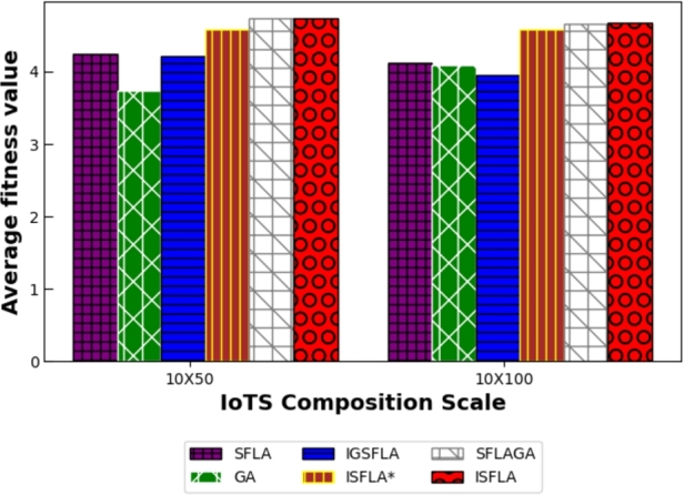
Comparison of the average optimal value when A=10.
Figure 7.
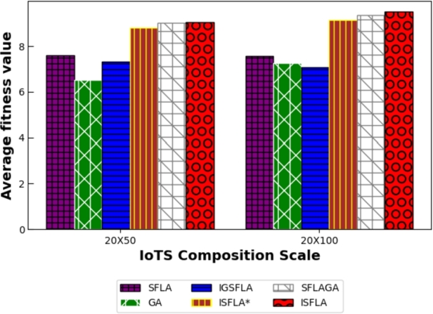
Comparison of the average optimal value when A=20.
Figure 8.
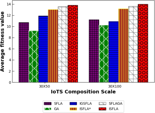
Comparison of the average optimal value when A=30.
5.3.2. Analysis of convergence of the algorithm
The second is the convergence of the algorithm. The experiment is also carried out under the above IoTS scale, as shown in Fig. 9 to Fig. 11 results. Under different scales of IoTS composition, with the increase of the number of global iterations, the average optimal value of IoTS composition gradually increases, and all algorithms on the graph basically reach convergence within 200 iterations. In Fig. 9, when A=10 in the IoTS scale, ISFLA can not only obtain the average fitness value not lower than other algorithms on the graph, but also converge faster than other algorithms. For example, although the average fitness value obtained by ISFLA is not significantly higher than that of SFLAGA, it reaches convergence significantly faster than SFLAGA. The global iteration times of ISFLA are about 50, while that of SFLAGA is about 100. Compared with ISFLA*, although the difference in convergence speed between the two is not very large, the average fitness value obtained by ISFLA is significantly higher than that of ISFLA*. Compared with SFLA, GA and IGSFLA, ISFLA is superior in average fitness value and convergence speed. In Fig. 10, when A=20 in the IoTS scale, ISFLA is still larger than other algorithms on the graph in the average fitness value, and the average fitness value of ISFLA is larger than SFLAGA to a larger extent. In terms of convergence speed, the advantage of ISFLA over other algorithms is not obvious, but ISFLA can get better average fitness value. In Fig. 11, when A=30 in the IoTS scale, compared with SFLAGA, the advantage of the average fitness value obtained by ISFLA becomes larger again, and the convergence speed is better. Compared with other algorithms on the graph, although ISFLA does not have an obvious advantage in convergence speed, the average fitness value obtained by ISFLA shows an obvious advantage. It can be seen that with the increase of the scale of IoTS, the advantages of ISFLA gradually become larger. In summary, it can be concluded that ISFLA has relatively better convergence performance.
Figure 9.

Comparison of convergence of average optimal values when A=10.
Figure 11.

Comparison of convergence of average optimal values when A=30.
Figure 10.

Comparison of convergence of average optimal values when A=20.
5.3.3. Analysis of stability of the algorithm
The third is the stability of the algorithm. The stability of the intelligent algorithm is the key to accurately obtain the best value in the face of complex problems. In order to show and analyze the stability of each algorithm in different scales of IoTS composition, the optimal fitness value list of each algorithm at each scale is obtained by searching each algorithm 100 times in three cases of different IoTS scales: 10×100, 20×100, 30×100, and then the standard deviation is calculated. The size of the standard deviation can judge the stability of the algorithm. Under the same conditions, the stability of different algorithms with smaller standard deviation is stronger, and vice versa is weaker. The standard deviation of each algorithm obtained by the experiment is shown in Table 4, and it can be seen that the standard deviation of ISFLA is significantly smaller than the standard deviation of other algorithms. With the continuous increase of the scale of IoTS, the standard deviation of each algorithm is increasing. The reason is that the stability of the algorithm is affected by the continuous expansion of the problem scale. It shows that the standard deviation of 30×100 scale is significantly larger than that of 20×100 or 10×100 scale. However, the standard deviation of ISFLA is still smaller than other algorithms. The results can also be seen in Fig. 12, where the abscissa is the different IoTS scales and the ordinate is the standard deviation of the optimal value obtained from 100 experiments. In summary, this indicates that ISFLA has better stability in obtaining the optimal solution.
Table 4.
Standard deviation for different IoTS scales.
| A | I | Standard deviation |
|||||
|---|---|---|---|---|---|---|---|
| ISFLA | SFLA | SFLAGA | IGSFLA | ISFLA* | GA | ||
| 10 | 100 | 0.0001154 | 0.0984059 | 0.0117937 | 0.0944845 | 0.0421759 | 0.084821 |
| 20 | 100 | 0.0177277 | 0.1739253 | 0.0592577 | 0.1228199 | 0.1034664 | 0.1186472 |
| 30 | 100 | 0.0430698 | 0.2967645 | 0.1000649 | 0.2507623 | 0.1621249 | 0.1570019 |
Figure 12.

Comparison of standard deviation.
5.3.4. Analysis of runtime of the algorithm
Finally, the runtime of the algorithm. The runtime of the algorithm refers to the time required for the algorithm to complete an experimental simulation. In this group of experiments, each algorithm was tested under the same experimental parameters, and 500 experimental simulations were carried out under different IoT service scales of 10×100, 20×100 and 30×100, and the average runtime of each algorithm was obtained. The results are shown in Table 5. Under the same experimental parameters and data set, ISFLA consumes more time at execution time. The reason is that in ISFLA, the local search of each group requires 20 local searches, and each local search is supplemented by the cross-variation of individual iterations in the group. As a result, ISFLA consumes more time, while GA and SFLAGA algorithms do not carry out more local searches. So they take less time than ISFLA. The difference in runtime between ISFLA and other algorithms is small. However, under the premise of obtaining a better optimal solution, the time consumed is within the acceptable range. Therefore, in order to make the algorithm achieve better performance in effectiveness, stability and convergence speed, it is worthwhile to sacrifice a small amount of time, and in general, ISFLA is superior.
Table 5.
Runtime for different IoTS scales.
| A | I | Runtime (s) |
|||||
|---|---|---|---|---|---|---|---|
| ISFLA | SFLA | SFLAGA | IGSFLA | ISFLA* | GA | ||
| 10 | 100 | 4.4151 | 5.6531 | 2.2168 | 5.5352 | 4.6226 | 1.7712 |
| 20 | 100 | 5.1344 | 6.1739 | 2.5881 | 6.3019 | 5.9902 | 1.9731 |
| 30 | 100 | 6.4454 | 7.2967 | 2.8218 | 7.2507 | 6.5204 | 2.1079 |
In summary, when ISFLA is looking for the optimal fitness value, compared with the compared algorithms, ISFLA can find a better fitness value with faster convergence speed, that is, it can find a better IoTS composition scheme. And with the growing scale of IoTS, the advantages of ISFLA are gradually increasing. In terms of the stability of the solution, ISFLA is more stable than other algorithms. Therefore, the convergence of ISFLA is better, the stability is better, and the comprehensive operation efficiency of ISFLA algorithm is higher. It is verified that the proposed method can obtain the IoTS composition that fulfills the user's non-functional requirements, and can effectively solve the large-scale IoTS composition problem.
6. Concluding
The optimization problem of IoTS composition is a current hotspot in research. This paper introduces the problem description of QoS-based IoTS composition and outlines the overall experimental process for solving the problem. To enhance the efficiency and accuracy of solving the optimization problem in IoTS composition using intelligent algorithms, this paper proposes improvements to the original SFLA. In the population initialization, Logistics chaotic mapping and reverse learning are introduced to generate the initial population. The group partitioning is done by calculating Euclidean distances. The global search incorporates a Gaussian mutation operator for evolving the optimal individual. The local update phase employs a strategy based on mutual learning, selection, crossover, and mutation for updating evolution. Finally, the improved algorithm is applied to IoTS composition optimization, effectively addressing the optimization problem in composing IoTS and obtaining approximately optimal solutions. Experimental results indicate that, compared to SFLA, GA, ISFLA*, IGSFLA and SFLAGA, the ISFLA consistently yields superior optimal solutions under the same experimental conditions. It further improves optimization accuracy, the quality of optimal solutions, and stability. In terms of algorithm runtime, the ISFLA exhibits advantages in efficiency without significant drawbacks. However, the paper has some limitations, including the absence of a rational analysis and dynamic calculation of QoS attribute weights and insufficient consideration of constraints between IoTS and variations in service performance in complex IoT dynamic environments, the ISFLA still has some disadvantages in runtime that need to be improved. For future work, we plan to dynamically calculate QoS attribute weights based on IoTS demands and increase the types of QoS attributes. We will also consider constraints between IoTSs and the dynamic environmental changes affecting service performance in IoTS composition optimization. Additionally, we will further analyze factors influencing the performance of the SFLA to enhance its overall performance. This will enable the selection of IoTS compositions that better meet user non-functional requirements in the contemporary IoT environment.
CRediT authorship contribution statement
Zhengyi Tang: Writing – review & editing, Writing – original draft, Validation, Methodology, Data curation, Conceptualization. Yongbing Wu: Writing – review & editing, Writing – original draft, Methodology, Formal analysis. Jinshui Wang: Writing – review & editing, Validation, Project administration, Data curation. Tianwei Ma: Writing – review & editing, Supervision, Formal analysis.
Declaration of Competing Interest
The authors declare that they have no known competing financial interests or personal relationships that could have appeared to influence the work reported in this paper.
Data availability
The data that support the findings of this study are available in IoTS_Dataset: QoS data about IoT services at https://zenodo.org/records/10440967, DOI 10.5281/zenodo.10440966. These data are generated within the limits by a randomized algorithm.
References
- 1.Guinard Dominique, Trifa Vlad, Karnouskos Stamatis, Spiess Patrik, Savio Domnic. Interacting with the soa-based Internet of things: discovery, query, selection, and on-demand provisioning of web services. IEEE Trans. Serv. Comput. 2010;3(3):223–235. [Google Scholar]
- 2.Chen Ray, Guo Jia, Bao Fenye. Trust management for soa-based iot and its application to service composition. IEEE Trans. Serv. Comput. 2014;9(3):482–495. [Google Scholar]
- 3.La Hyun Jung, Kim Soo Dong. 2010 IEEE/ACIS 9th International Conference on Computer and Information Science. IEEE; 2010. A service-based approach to designing cyber physical systems; pp. 895–900. [Google Scholar]
- 4.Piyare Rajeev, Lee Seong Ro. Towards Internet of things (iots): integration of wireless sensor network to cloud services for data collection and sharing. 2013. arXiv:1310.2095 arXiv preprint.
- 5.Wu Hongyue, Du Yu-Yue. A logical petri net-based approach for web service cluster composition. Chinese J. Comput. 2015;38(1):204–218. [Google Scholar]
- 6.Hamed Bouzary, Chen F. Frank. A classification-based approach for integrated service matching and composition in cloud manufacturing. Robot. Comput.-Integr. Manuf. 2020;66 [Google Scholar]
- 7.Jatoth Chandrashekar, Gangadharan G.R., Fiore Ugo. Optimal fitness aware cloud service composition using modified invasive weed optimization. Swarm Evol. Comput. 2019;44:1073–1091. [Google Scholar]
- 8.Baker Thar, Asim Muhammad, Tawfik Hissam, Aldawsari Bandar, Buyya Rajkumar. An energy-aware service composition algorithm for multiple cloud-based iot applications. J. Netw. Comput. Appl. 2017;89:96–108. [Google Scholar]
- 9.Ma Shang-Pin, Lin Hsuan-Ju, Hsu Ming-Jen. Semantic restful service composition using task specification. Int. J. Softw. Eng. Knowl. Eng. 2020;30(06):835–857. [Google Scholar]
- 10.Yaghoubi Mohamadali, Maroosi Ali. Simulation and modeling of an improved multi-verse optimization algorithm for qos-aware web service composition with service level agreements in the cloud environments. Simul. Model. Pract. Theory. 2020;103 [Google Scholar]
- 11.Zhang Lei. Hangzhou Dianzi University; 2019. Research on automatic web service composition method based on keyword search. Master's thesis. [Google Scholar]
- 12.Jaeger Michael C., Muhl Gero, Golze Sebastian. IEEE International Conference on Web Services (ICWS'05) IEEE; 2005. Qos-aware composition of web services: a look at selection algorithms. [Google Scholar]
- 13.Ren Ping. Genetic algorithms (an overview) Chin. J. Eng. Math. 1999;16(1):1–8. [Google Scholar]
- 14.Hassan Bryar A. Cscf: a chaotic sine cosine firefly algorithm for practical application problems. Neural Comput. Appl. 2021;33(12):7011–7030. [Google Scholar]
- 15.Qader Shko M., Hassan Bryar A., Rashid Tarik A. An improved deep convolutional neural network by using hybrid optimization algorithms to detect and classify brain tumor using augmented mri images. Multimed. Tools Appl. 2022;81(30):44059–44086. [Google Scholar]
- 16.Ghaemi Amir, Arasteh Bahman. Sfla-based heuristic method to generate software structural test data. J. Softw. Evol. Process. 2020;32(1) [Google Scholar]
- 17.Arasteh Bahman, Sadegi Razieh, Arasteh Keyvan. Bölen: software module clustering method using the combination of shuffled frog leaping and genetic algorithm. Data Technol. Appl. 2021;55(2):251–279. [Google Scholar]
- 18.Arasteh Bahman, Karimi Mohammad Bagher, Sadegi Razieh. Düzen: generating the structural model from the software source code using shuffled frog leaping algorithm. Neural Comput. Appl. 2023;35(3):2487–2502. [Google Scholar]
- 19.Xiao Yuanyuan, Xu Xuemin, Zhang Xiuguo, Cao Zhiying. Large-scale web service composition based on improved grey wolf optimizer algorithm. J. Comput. Appl. 2022;42(10):3162. [Google Scholar]
- 20.Xue Fucheng, Yang Hongwei, Li Li. Web service composition based on sparrow search algorithm. Comput. Eng. Des. 2022 [Google Scholar]
- 21.Tan Wenan, Zhao Yao. Web service composition based on chaos genetic algorithm. Comput. Integr. Manuf. Syst. 2018;24(07):1822. [Google Scholar]
- 22.Liu Xingchen, Liao Shuichong, Sun Peng, Zhong Yun. Service composition optimization based on improved krill herd algorithm. J. Comput. Appl. 2021;41(12):3652. [Google Scholar]
- 23.Tan Wenan, Wu Jiakai. Optimization of web service composition based on improved flower pollination algorithm. Comput. Eng. 2020 [Google Scholar]
- 24.Chen Zhipo, Ouyang Chao, Sun Guodong. Improved genetic algorithm for web service composition qos optimization. Comput. Eng. 2017;34(8):231–235. [Google Scholar]
- 25.Asghari Parvaneh, Rahmani Amir Masoud, Haj Hamid, Javadi Seyyed. Privacy-aware cloud service composition based on qos optimization in Internet of things. J. Ambient Intell. Humaniz. Comput. 2020:1–26. [Google Scholar]
- 26.Guo Haowen, Sun Yuzhen, Huang Xiaoxiao. Optimization of coordinated control system basedon improved shuffled frog leaping algorithm. J. Eng. Therm. Energy Power. 2020;35(6) [Google Scholar]
- 27.Bakhshi Mahdi, Hashemi Mohsen. User-centric optimization for constraint web service composition using a fuzzy-guided genetic algorithm system. 2012. arXiv:1210.3604 arXiv preprint.
- 28.Maaroof Bestan B., Rashid Tarik A., Abdulla Jaza M., Hassan Bryar A., Alsadoon Abeer, Mohamadi M., Mirjalili S. Current studies and applications of shuffled frog leaping algorithm: a review. Arch. Comput. Methods Eng. 2022;2(1):1–16. [Google Scholar]
- 29.Zhao Junjie, Tan Faming, Wang Qi. A grey wolf optimization algorithm with improved nonlinear convergence. Microelectron. Comput. 2019;5:89–95. [Google Scholar]
- 30.Chen Jiaqing, Shi Mohan, Gao Chenfeng. Bald eagle search algorithm based on chaotic map and adaptive opposition-based learning. Math. Pract. Theory. 2022;52(6):11. [Google Scholar]
- 31.Ji Weidong, Ni Wanlu. A dynamic control method of population size based on Euclidean distance. J. Electron. Inf. Technol. 2022;44(6):2195–2206. [Google Scholar]
- 32.Fang Yangwang, Yan Xiaobin, Peng Weishi. Multi-objective harris hawk optimization algorithm based on adaptive gaussian mutation. J. Beijing Univ. Aeronaut. Astronaut. 2022;48 [Google Scholar]
Associated Data
This section collects any data citations, data availability statements, or supplementary materials included in this article.
Data Availability Statement
The data that support the findings of this study are available in IoTS_Dataset: QoS data about IoT services at https://zenodo.org/records/10440967, DOI 10.5281/zenodo.10440966. These data are generated within the limits by a randomized algorithm.