A kV-MV approach to CBCT metal artifact reduction using multi-layer MV-CBCT

Abstract

Objective:

To demonstrate that complete cone beam CT (CBCT) scans from both MV-energy and kV-energy LINAC sources can reduce metal artifacts in radiotherapy guidance, while maintaining standard-of-care x-ray doses levels.

Approach:

MV-CBCT and kV-CBCT scans are acquired at half normal dose. The impact of lowered dose on MV-CBCT data quality is mitigated by the use of a 4-layer MV-imager prototype and reduced LINAC energy settings (2.5 MV) to improve photon capture. Additionally, the MV-CBCT is used to determine the 3D position and pose of metal implants, which in turn is used to guide model-based poly-energetic correction and interleaving of the kV-CBCT and MV-CBCT data. Certain edge-preserving regularization steps incorporated into the model-based correction algorithm further reduce MV data noise.

Main Results:

The method was tested in digital phantoms and a real pelvis phantom with large 2.5” spherical inserts, emulating hip replacements of different materials. The proposed method demonstrated an appealing compromise between the high contrast of kV-CBCT and low artifact content of MV-CBCT. Contrast-to-noise improved 3-fold compared to MV-CBCT with a clinical 1-layer architecture at matched dose (37 mGy) and edge blur levels. Visual delineation of the bladder and prostate improved noteably over kV- or MV-CBCT alone.

Significance:

The proposed method demonstrates that a full MV-CBCT scan can be combined with kV-CBCT to reduce metal artifacts without resorting to complicated beam collimation strategies to limit the MV-CBCT dose contribution. Additionally, significant improvements in CNR can be achieved as compared to metal artifact reduction through current clinical MV-CBCT practices.

1. Introduction

Cone beam CT (CBCT) has been used commonly as a means of image guidance in external beam radiation therapy (EBRT). In patients containing metal prosthetic implants, CBCTs at traditional kV-range x-ray energies can exhibit severe artifacts when standard image reconstruction techniques such as FDK (Feldkamp et al 1984) are used. These artifacts obscure anatomy of interest in the area of the treatment site, impeding targeting and registration with prior planning CTs in conventional EBRT. Likewise, such artifacts are a problem for on-treatment organ segmentation and tumor contouring for adaptive radiotherapy (ART) practices.

One means of mitigating metal artifacts that has appeared in radiotherapy clinics is the use of MV-range x-ray energies, generated by the LINAC source, for 3D image guidance. Systems employing 3D MV imaging include Varian’s Halcyon system and Accuray’s Radixact. Owing to the higher tissue penetration of MV photons, metal artifact content in MV images is greatly reduced. Conducting 3D MV scans at acceptable radiation doses has been challenging, in part due to the restricted x-ray energy settings available on commercial LINACs, typically no lower than 6 MVp. In more recent years, however, methods for generating lower energy LINAC output (Faddegon et al 2008, Tang et al 2016) have emerged. In developer mode, Varian’s Edge LINAC can acquire MV-CBCT data at 2.5 MVp, while the Radixact has a clinically available MVCT feature operating at 3.5 MV. In spite of these advancements, x-ray detection efficiency is still challenged at such high energies, and therefore MV imaging noise tends to be considerably higher than kV-CBCT.

As an alternative to MV imaging, considerable prior work (Stayman et al 2012a, Zhang et al 2017, Xu et al 2017, Stayman et al 2012b) has demonstrated improvements in kV-CBCT image reconstruction quality when the presence of metal in the patient can be explicitly modeled into the reconstruction process. Such advanced methods, however, require that the shape, material composition, and geometric pose be determined either a priori, or else co-estimated in the course of the reconstruction. Thanks to modern advances in medical record-keeping, the shape and material composition of a prosthetic implant are often traceable from individual patient records, making those less problematic in model-based metal artifact reduction (MAR). However, the specific pose and position of an implant within the patient anatomy are not available off-line, and must be determined at scan time. In prior literature, multiple ways of localizing patient implants from the given kV-CBCT have been offered. In some work, the implants are segmented directly from a preliminary, non-corrected kV-CBCT reconstruction (Rinkel et al 2008, Yazdia et al 2005). Because the preliminary kV-CBCT is artifacted, it may be challenging to select a segmentation threshold that delineates the implant boundaries accurately. Consequently, some work has proposed to register a prior geometric model of the implant to the measured projection data (Uneri et al 2019). Still other work proposes to model the implant pose using additional unknown variables that are co-reconstructed with the unknown voxel values as part of the reconstruction process (Stayman et al 2012a).

Other prior works (Wu et al 2014, Lindsay et al 2019) have also looked at ways to reduce metal artifacts using hybrids of kV and MV data. So called kV-MV methods take advantage of the fact that many EBRT systems are dual-source imaging systems, where both kV-CBCT and MV-CBCT data are available. In doing so, it is hoped that the final image quality will offer a favorable compromise between the high CNR of kV-CBCT and the low artifact content of MV-CBCT. With such approaches, it is common to try to overpaint the metal-affected kV projection pixels with less photon-starved MV data, and then to reconstruct a reduced-artifact volume from the interleaved data. A limitation with previous kV-MV proposals is that, at the time of that work, only 6 MVp energy levels were common on LINACs. Therefore, to achieve acceptable x-ray doses, it was necessary to employ complicated source collimation strategies that limit the MV beam exposure to metal-affected regions of the patient. This means that a complete MV-CBCT volume could not be reconstructed.

By contrast, this paper proposes a kV-MV method that leverages a complete three-dimensional MV-CBCT acquisition. Moreover, it does so while at the same time restricting total dose to that of a conventional kV-CBCT. The method is able to do so in part due to (a) the use of lower 2.5 MV exposure settings now available (b) a noise-suppressing poly-energetic correction method adapted from previous work (see Section 2.3), and (c) the use of a 4-layer, high efficiency MV-imager to improve data quality. The MV imager design was previously analyzed for 2D performance (Jacobson et al 2021) and was found to improve detected quantum efficiency (DQE) by at least a factor of 3 compared to detector architectures in clinical use. It was also shown to be beneficial to 3D CBCT imaging performance with metal-free CBCT subjects. The availability of a complete prior MV-CBCT volume is advantageous firstly because it eliminates the need for dynamic source collimation. Second, it allows for accurate determination of the position and pose of metal prosthetics, due to its low artifact content, thereby facilitating model-based beam hardening correction. Third, the 3D MV-CBCT volume can be reprojected into the metal-affected regions of the kV-CBCT projections. We find empirically that this improves the quality of projection overpainting when uncorrected scatter is present. An additional novel aspect of our approach is that we use the prior MV-CBCT to determine the metal thickness seen by different regions of the kV-CBCT data, and to choose which projection views to overpaint based on these differences.

In the remainder of the paper, the overall technique is tested both in simulation and on real data acquired with Varian’s Edge LINAC. For the real data experiments, a custom pelvis phantom is used with 2.5” spherical slots in the femoral heads, allowing simulated hip replacements of different materials to be tested. Imaging performance was assessed in terms of contrast-to-noise ratio between muscle and adipose tissue, as well as in terms of artifact content, which was quantified using a two-region uniformity metric. The proposed kV-MV method outperformed 1-layer MV-CBCT with respect to CNR, and exhibited an appealing compromise between the high CNR of standard kV-CBCT and low metal artifact content of standard MV-CBCT.

2. Materials and Methods

2.1. kV-MV Acquisition Strategy with Multi-Layer MV Imager

Figure 1 summarizes the kV-MV acquisition technique and system components that were examined in this paper. The MV-CBCT component used a prototype multi-layer imager (MLI) consisting of 4 layers, each similar to the Varian Halcyon system, except that no copper filter layers are used. Each layer consisted of two main sub-layers, a GOS scintillator (GdO₂S₂:Tb) and an aSi:H photodiode/TFT-switch with a glass substrate, having respective area densities of 2.00 mg/mm² and 1.62 mg/mm². In prior work (Jacobson et al 2021), it was shown that this architecture increases DQE(0) by at least a factor of 3 for both 2.5 MV FFF and 6 MV FFF beams.

Figure 1:

Drawing of the KV-MV scan geometry and system components, including the prototype multi-layer MV detector architecture.

In a clinical implementation of the kV-MV method, both kV and MV projections would be acquired concurrently during gantry rotation, but with out-of-phase irradiation pulses so as to minimize scatter cross-contamination. For the sake of prototyping simplicity, however, kV-MV acquisitions were synthesized in the present study by combining projection view subsets from separate 360° kV-CBCT and MV-CBCT scans, both collected using a Varian Edge^™ radiotherapy sytem. The source-isocenter distance and source-detector distance were 100 cm and 150 cm, respectively, for both the kV and MV imagers, while the detector dimensions were 40 cm × 30 cm and 43 cm × 43 cm, respectively. The kV-CBCT acquisition settings were that of Varian’s clinical “Large Pelvis” half-fan protocol (360°/900 views, 140 kVp, 1688 mAs), while the MV-CBCT projections were acquired with experimental LINAC settings (360°/720 views, 2.5 MV FFF, 8 MU) in full-fan position. Based on prior CTDI measurements, the kV and MV scans both delivered doses of approximately 37 mGy. All acquired projection views underwent flood-field, dark-field, and scatter-removal pre-corrections. Scatter correction used the fASKS kernel-based algorithm (Sun and Star-Lack 2010), as implemented in Varian’s proprietary iTools Reconstruction software package.

2.2. Overall kV-MV Data Processing Chain

The overarching steps of the kV-MV data processing chain are show in Figure 2(a). Beginning with kV and MV projection data sets $Y_{\mathrm{k}\mathrm{V}}$ and $Y_{\mathrm{M}\mathrm{V}}$, the processing starts with a preliminary reconstruction of the MV-CBCT projections. The 3D reconstruction is then segmented by simple thresholding to obtain the spatial distribution of metal in the patient. Here, the material composition of the metal is assumed known from patient records while the prior segmentation map is used to determine its position, shape, and pose at scan time. The spatial distribution of metal is then forward projected to obtain the path length $t_i$ of the metal along each measured x-ray path, $i$, through the patient.

Figure 2:

Elements of the proposed kV-MV data processing technique (a) High level flow diagram for overall kV-MV processing chain, illustrated for a phantom with bilateral metal inserts in the femoral heads. (b) Measurement model for RPME poly-energetic correction method. (c) Selective over-painting of RPME-corrected kV data with MV data.

We then apply an algorithm (see Section 2.3 and Figure 2(b)) that we call Roughness Penalized Mono-energization (RPME). The RPME algorithm is a poly-energetic correction technique which determines the contribution of water-equivalent material $w_i$ to x-ray path $i$, based on the known emission spectrum of the x-ray source. The contribution of metal $t_i$ is treated as known from the above-mentioned segmentation step. By applying RPME to both the kV- and MV-CBCT measurements, projection data sets ${\widehat{w}}_{kV}$ and ${\widehat{w}}_{MV}$ are obtained, representing the estimated pathlengths of water-equivalent material from the perspectives of the kV and MV imagers.

In a third step, the pre-determined metal path lengths $t_i$ are used to identify projection angles containing particularly high metal attenuation. If a projection view of ${\widehat{w}}_{kV}$ contains pixels with $t_i$ exceeding a user-selected threshold, T, the metal-affected pixels in that projection view are over-painted (see Figure 2(c)) with interpolated pixel values from ${\widehat{w}}_{MV}$ to eliminate photon-starved pixel values. Because the water-equivalent path lengths are weakly dependent on energy (for a water-phantom, they are completely independent), this data interleaving can be done with minimal inconsistency among the pixel values of the resulting projections, which are denoted ${\widehat{w}}_{kV/MV}$. Finally, the two data sets ${\widehat{w}}_{kV/MV}$ and ${\widehat{w}}_{MV}$ are reconstructed (with FDK) to obtain virtual mono-energetic images (VMIs) at a reference energy $E_0$ taken throughout this paper as 65 keV (the average detected energy of the Edge LINAC’s kV x-ray source). The two VMIs are averaged together to obtain a final 3D image. Because ${\widehat{w}}_{MV}$ and ${\widehat{w}}_{kV/MV}$ account for only water-equivalent material, metal objects will be absent in this final image, but can easily be re-inserted digitally using the prior metal segmentation map from above, if desired.

2.3. Roughness Penalized Mono-energization (as applied to Metal Artifact Reduction)

The RPME technique was introduced in (Jacobson et al 2021) which in turn was based on the works of (Joseph and Spital 1978) and (La Rivière et al 2006, La Rivière and Pan 2000, La Rivière 2005). Here, we describe its adaptation to the metal artefact reduction problem considered in this paper. The RPME algorithm models the projected attenuation measured in the $i$-th pixel as the contribution of two basis materials, one of them water, with energy-dependent attenuation ${\mu }_w\left(E\right)$, and the other a higher attenuation material of known 3D spatial distribution. In (Jacobson et al 2021), the basis materials were chosen to be bone and water, where the distribution of bone was pre-estimated from a primitive initial reconstruction using the method of (Joseph and Spital 1978). In this paper, the higher attenuating material is metal, while the entirety of the natural patient anatomy is approximated as water. The type of metal chosen for the model is based on prior knowledge of the implant characteristics from patient records. The spatial distribution of the metal, as mentioned earlier, is determined from pre-segmentation of an MV-CBCT.

Denoting the metal attenuation as ${\mu }_t\left(E\right)$, this leads to the following poly-energetic model equation (see also Figure 2(b)) for the mean of the $i$-th projection measurement $Y_i$ (after gain, offset, and scatter pre-corrections),

$$y_i\left(w_i\right)={\sum }_{E}E{I}_i(E)\text{exp}\left(\text{-}{w}_i{\mu }_w(E)\text{-}{t}_i{\mu }_t(E)\right)$$ Eq. 1

Here, $w_i$ is the unknown water-equivalent path length to be estimated, while $t_i$ is the known path length of metal seen by the pixel. The coefficients $I_i\left(E\right)$ denote the proportion of photons with energy $E$ that are absorbed in the detector and are normalized here so that ${\sum }_{E}E{I}_i(E)=1$, consistent with the fact that the projections are gain corrected. The spectra $I_i\left(E\right)$ vary with $i$ according to whether that ray was captured with the kV-CBCT or the MV-CBCT imager. In the case of a kV-imager measurement, $I_i\left(E\right)$ also varies spatially across the detector due to the non-uniform cross-section of the bowtie filter.

Given the model in Eq. 1, we estimate the $w_i$ by minimizing a penalized Poisson likelihood function,

$$\text{min}.{\sum }_i{y}_i\left(w_i\right)\text{-}{Y}_i\text{log}\left(y_i\left(w_i\right)\right)+\beta H_{\delta }(w).$$ Eq. 2

where $H_{\delta }\left(w\right)$ is the edge-preserving Huber loss,

$$H_{\delta }(w)={\sum }_i{\sum }_{j\in {𝒩}_i}{\alpha }_j{h}_{\delta }\left(w_i\text{-}{w}_j\right)$$

$$h_{\delta }(z)=\{\begin{array}{ll}\frac{1}{2}{z}^2\hfill & |z|\le \delta \hfill \\ \delta \left(|z|-\frac{1}{2}\delta \right)\hfill & |z|>\delta .\hfill \end{array}$$

The parameter $\beta >0$ is a regularization weight, $\delta >0$ is an edge threshold parameter, and ${𝒩}_i$ are the neighboring pixels around $i$ when the measurements $Y_i$ are organized as a 3D array. The coefficients ${\alpha }_j$ represent weights applied to the different pixel differences $w_i\text{-}{w}_j$. An iterative algorithm for minimizing Eq. 2 was presented in (Jacobson et al 2021) and follows the update formula,

$$w_i^{n+1}=\left\{z|\frac{Y_i}{y_i(w_i^n)}{\dot{y}}_i(w_i^n)-{\dot{y}}_i(z)-2(z\text{-}{w}_i^n)\left[{\sum }_{j\in {𝒩}_i}{q}_{\delta }\left(w_i^n\text{-}{w}_j^n\right)-{\sum }_{j\in {𝒩}_i}{\alpha }_j{\dot{h}}_{\delta }\left(w_i^n\text{-}{w}_j^n\right)\right]=0\right\}$$ Eq. 3

Note that these updates are performed per-pixel and so are well-suited to GPU parallelization. Furthermore, they operate entirely in the projection domain and involve no iterative forward and back projection.

2.4. Inpainting

In this section, we describe the inpainting process, shown in Figure 2(a) and (c), in somewhat more detail. As mentioned earlier, the water-equivalent thicknesses $w_i$ are approximately the same for kV and MV projections obeying equation Eq. 1. This facilitates smooth inter-splicing of the two data sets. However, realistic projections deviate somewhat from this ideal model, for example because of residual uncorrected scatter. Therefore, some additional steps are adopted during the inpainting process as empirical corrections. The overall steps of the inpainting are as follows:

1. Affine Correction: the Overlap Based Projection Rescaling (OBPR) method is applied, wherein we fit a linear relation ${\widehat{w}}_{kV}=a{\widehat{w}}_{MV}+b$. This method is originally due to (Yin et al 2005), although the name OBPR was coined by us, for convenience. It involves fitting coefficients $a$ and $b$ based on pixel values from a small number of approximately overlapping kV and MV projection views, interpolated to have the same frame dimensions (see Figure 4). Once this fit is achieved, it is used to transform the total set of projection views in ${\widehat{w}}_{MV}$ into new projections, ${\widehat{w}}_{MV}^{\ast }$. The transformed pixel intensities are closer to true kV data, and so are more suitable for filling in missing or degraded pixel values. In our application of OBPR, 10 projections from ${\widehat{w}}_{kV}$ and ${\widehat{w}}_{MV}$ were used for the fit. Pixels that were metal-affected or which lay outside the field of view (FOV) of either detector were excluded.

2. Reprojection: As a further correction, the transformed projections ${\widehat{w}}_{MV}^{\ast }$ are FDK-reconstructed and then reprojected to obtain a new set of projections ${\widehat{w}}_{MV}^{\ast \ast }$. If specific projection views of ${\widehat{w}}_{MV}^{\ast }$ have higher residual scatter contamination than the others, this reprojection step tends to dilute the contamination over many views, further mitigating artifacts.

3. Projection Resampling: At this point, we have a set of projections ${\widehat{w}}_{MV}^{\ast \ast }$ that we would like to use to overpaint metal-affected pixels in another data set ${\widehat{w}}_{kV}$. However, the projection views in each data set correspond to a different sequence of LINAC gantry angles ${\mathrm{\theta }}_{kV}$ and ${\mathrm{\theta }}_{MV}^{\ast \ast }$. We transform ${\widehat{w}}_{MV}^{\ast \ast }$ by linearly interpolating its pixel values according to gantry angle, querying at angles ${\mathrm{\theta }}_{kV}$. The spatial pixel coordinates are likewise interpolated to match those of ${\widehat{w}}_{kV}$. This results in a third set of transformed projections ${\widehat{w}}_{MV}^{\ast \ast \ast }$ having the same source-detector geometry as ${\widehat{w}}_{kV}$.

4. Overwrite kV Pixels: Metal-affected pixel values from ${\widehat{w}}_{MV}^{\ast \ast \ast }$ are inserted into the corresponding pixel locations in ${\widehat{w}}_{kV}$ giving the final result, ${\widehat{w}}_{kV/MV}$. If all metal-affected pixels in a certain projection view see metal thicknesses below the chosen threshold (i.e., $t_i\text{<}\mathrm{T}$), then that projection view is omitted from the inpainting step. To mitigate discontinuities at the edges of the inpainted regions, each row of pixels in the overpainted views is processed according to,

   $${\widehat{w}}_{kV/MV}=\{\begin{array}{ll}{\widehat{w}}_{MV}^{\ast \ast }+\text{F}({\widehat{w}}_{kV})-\text{F}({\widehat{w}}_{MV}^{\ast \ast \ast })\hfill & t_i>0\hfill \\ {\widehat{w}}_{kV}\hfill & t_i=0\hfill \end{array}$$

   Here $\mathrm{F}(\cdot )$ represents linear interpolation-based filling of the metal-affected pixels, as implemented by MATLAB’s fillmissing command.

Figure 4:

Depiction of the OBPR method, due to (Yin, Guan and Lu, 2005) in which a linear fit to over-lapping kV and MV projection views is used to transform MV pixel values into approximately equivalent kV pixel values. The transformed pixel values can then be more readily inter-spliced with actual kV data, to fill in missing or degraded pixel values.

It is important to note that the affine correction and reprojection steps above are unnecessary in data that is well scatter-corrected and for which the x-ray source spectra are accurately known. We do include these steps, however, in our scatter-free simulation experiments described in the next section.

2.5. Simulation Experiments

Preliminary simulation tests of the method were made to assess performance in the ideal case of a perfectly accurate beam spectrum model and no scatter. Simulated kV- and 4-layer MV-CBCT projections were generated for the digital phantoms in Figure 3(a) and 3(b). The digital pelvis in Figure 3(a) contained a titanium right hip. The thorax phantom in Figure 3(b) contained two titanium pedicle screws enclosing a cold lesion in the vertebra, made to resemble certain metastatic tumors sometimes observed in the clinic. In these phantoms, adipose tissue, muscle tissue, and trabecular and cortical bone were modeled to have the same chemical compositions as the real phantom from CIRS Inc. shown in Figure 3(c). The metastatic lesion was modeled as a 50:50 mixture of water and trabecular bone.

Figure 3:

Simulated and real phantom apparatus. (a) Digital pelvis phantom with titanium hip replacement (b) Digital thorax phantom with two titanium pedicle screws enclosing a cold lesion in the vertebra (c) Real pelvis phantom with interchangeable spherical inserts in the femoral heads. This is a custom modification of the CIRS-801-P-F phantom from Computerized Imaging Reference Systems, Inc.

In generating the simulated CBCT measurements, mean projections were first generated according to,

$$y_i={\sum }_{E}E{I}_i(E)\text{exp}\left(-{\sum }_m{l}_{im}{\mu }_m(E)\right)$$

where $l_{im}$ denotes the path length of the $m$-th material region of the digital phantom seen by the $i$-th pixel measurement. Poisson noise was then added so that FDK-reconstructed image noise levels were the same as those seen in the soft tissue regions of actual phantom scans at 25 mGy. The geometry for the data simulation was as in Figure 1. X-ray source energies were 125 kVp for the kV data and 2.5 MV FFF for the MV data. Data for simulating the emitted x-ray spectra were as published by Varian for the Edge LINAC system.

The proposed kV-MV technique was applied to these simulations with parameters $\beta =5.83\mathrm{e}\text{-}6$ and $\delta =4\mathrm{m}\mathrm{m}$. Neighborhood weights ${\alpha }_j=1$ were used for neighboring pixels within and between projection views. As noted in Section 2.6, these parameter choices were found to produce edge blur approximately matching baseline imaging techniques in real phantom scans. For the digital thorax, the kV-MV technique was applied with both an over-painting threshold parameter of $\mathrm{T}\text{=}0\mathrm{m}\mathrm{m}$ and of $\mathrm{T}\text{=}40\mathrm{m}\mathrm{m}$. The $\mathrm{T}\text{=}0\mathrm{m}\mathrm{m}$ case corresponds to overpainting all metal-affected projections, whereas with $\mathrm{T}\text{=}40\mathrm{m}\mathrm{m}$ overpainting is applied only to kV-CBCT projection views that look down the long axis of the screws. For the digital pelvis, over-painting was applied with $\mathrm{T}\text{=}0\mathrm{m}\mathrm{m}$ only. When applying the kV-MV technique, the number of projection views was decimated by half so that the total dose from kV and MV exposure combined remained at 25 mGy.

The images resulting from the kV-MV technique were compared to standard FDK reconstructions of the kV-only and MV-only data sets as generated above. Additionally, we compared our kV-MV technique to two baseline metal artifact reduction methods. One method was the linear-interpolation based method proposed by (Kalender et al 1987). In this method, metal-affected projection pixels in the kV-CBCT acqusition are treated as missing data and are filled row-wise using linear interpolation of neighboring, non-missing pixels. The second baseline method is a kV-MV technique, where again the metal-affected pixels are treated as missing data. Unlike our proposed technique, however, the missing kV-CBCT pixels are inpainted with MV data using a more basic, pre-existing method for kV-MV data-splicing, namely OBPR from Figure 4. For the two baseline methods, we used the full, undecimated set of projection kV-CBCT views. A segmentation and reprojection of the kV-only FDK reconstruction were used to identify metal-affected regions of projection data. In applying the kV-MV-OBPR method, the only MV projection rays used were those through the metal affected regions of the object, similar to previous work (Wu et al 2014, Lindsay et al 2019). No additional data pre-correction steps other than log- and scatter-correction were applied, also similar to previous work (Yin et al 2005). In particular, no prior beam hardening correction was used.

All FDK reconstructions were made with a Hamming apodization filter with a cut-off at 70% Nyquist. The images from the different techniques were all reconstructed with (1 mm)³ voxel resolution and assessed qualitatively for trade-off in artifact reduction versus soft tissue contrast.

2.6. Real Data Experiments

Based on real acquisitions of the pelvis phantom in Figure 3(c), the kV-MV imaging technique was compared to conventional kV-CBCT (with and without metal present) as well as to MV-CBCT. This comparison was done with the MV-detector operated in both 1-layer and 4-layer mode to assess the impact of the multi-layer architecture. Note that the 1-layer mode corresponds to the architecture of Varian’s clinical Halcyon system (without copper filtering). The phantom was a customization of the CIRS-801-P-F from Computerized Imaging Reference Systems, Inc. As shown in the figure, the phantom contains 2.5 inch diameter spherical slots, allowing one to swap the natural anatomy of the femoral heads for metal inserts emulating unilateral or bilateral hip-replacements. Note that 2.5 inches is at the upper end of the size range seen in actual hip prosthetics. In these experiments, we considered the case of a bilateral hipreplacement with aluminum heads, as well as a unilateral hip-replacment with a titanium head.

Projection data were acquired as described in Section 2.1. The kV-MV technique was again applied with half the available projection views, so that all techniques were approximately dose-matched, here at 37 mGy. RPME parameters for the kV-MV data processing chain were as in the simulation experiments of Section 2.5 namely $\beta =5.83\mathrm{e}\text{-}6,\delta =4\mathrm{ }\mathrm{m}\mathrm{m},{\alpha }_j=1$. The inpainting thickness threshold T was chosen to be $\mathrm{T}\text{=}70\mathrm{m}\mathrm{m}$ for the aluminum bi-lateral insert configuration and $\mathrm{T}\text{=}0\mathrm{m}\mathrm{m}$ for the titanium unilateral insert. Parameters for FDK reconstructions were also the same as in the hip simulation experiments. A slight difference, however, was that conventional kV-CBCT reconstructions underwent an additional Gaussian post-filtering step. This was to equalize the spatial resolution of the kV-CBCT with the MV-CBCT images, as the latter was influenced by higher scintillator blur from the MV detector layers. It was verified that the resulting images were approximately resolution-matched according to the edge spread metric depicted in Figure 5(a). To calculate edge spread, we selected a rectangular volume of interest (VOI) which was 5 slices thick and straddled a muscle-adipose tissue boundary. The edge spread function (ESF) along the different rows of voxels in this VOI was modeled as a Gaussian error function with unknown parameters $a,b,c$, and ${\bar{x}}_i$. Here ${\bar{x}}_i$ denotes the position of the edge boundary in the $i$-th row of the VOI, while $a,b,c$ are assumed constant across the VOI. The parameter of interest is $c$ which governs the ESF width. All imaging techniques compared in these experiments were found to have $c$ parameter values varying by at most 1.5 mm, or in other words were equal to within 1.5 reconstructed voxel widths.

Figure 5:

Methods for quantitative analysis. (a) The ESF is computed using a parametric model fitted to parallel profiles through an edge-straddling ROI in the non-metal-affected region of the phantom. (b) Contrast-to-Noise CNR is computed from two ROIs lying adjacent to a muscle-adipose boundary also in a non-metal-affected slice superior to the femoral heads. (c) A percent similarity metric is computed from two ROIs in a metal-affected reconstructed slice, one in a highly artifacted region of the bladder, and the second in a relatively un-artifacted region with the same tissue type.

Imaging performances from the different techniques were compared in terms of both contrast-to-noise (CNR) and artifact content. CNR was measured, see Figure 5(b), from the voxel means ${\mu }_A,{\mu }_B$ and standard deviations ${\sigma }_A,{\sigma }_B$ of two rectangular regions of interest (ROIs) in the vicinity of a muscle-adipose boundary. The ROIs were drawn in a slice about 1 cm above the hip so that the CNR measurement would not be influenced by uncorrected metal streak artifacts. Artifact content was measured according to a percent similarity measure, defined in Figure 5(c), between a metal-affected, streak-prone ROI in the bladder and a relatively unartifacted background ROI of the same muscle tissue type. A polygonal, non-rectangular ROI was drawn in the bladder so as to include more voxels while conforming to the bladder’s boundaries. Uncertainties in the CNR and % Similarity calculations were determined by dividing the voxels in the ROIs into 10 subsets. The standard deviation in the CNR and % Similarities as computed from these subsets defined the uncertainty.

As a final experiment, we also repeated the kV-MV reconstructions for a sweep of different inpainting threshold parameters ranging from $\mathrm{T}\text{=}10\mathrm{m}\mathrm{m}$ to $\mathrm{T}\text{=}120\mathrm{m}\mathrm{m}$ and quantified the % Similarity. This allowed us to assess the impact of the T parameter on artifact control for the different implant configurations.

3. Results

3.1. Simulated Phantom Results

Reconstructed images for the digital pelvis are compared in Figure 6. As may be expected, the 125 kV scans, representing clinical practice, exhibited the highest metal artifact content. Conversely, the higher energy 2.5 MV scan was essentially free of metal artifacts, but exhibited lower soft tissue contrast. The baseline metal artifact reduction methods are completely non-iterative and therefore very fast computationally. While they certainly improved global tissue uniformity relative to the 125 kV scan, strong streak and shading artifacts were also introduced. Undoubtedly, the linear interpolation method struggles here because of the large cross-section of the implants, leading to large regions of missing data in the projections. Thus, it is difficult for the algorithm to restore missing data by interpolation alone. Residual artifacts from the kV-MV-OBPR are not as strong as for linear interpolation, likely because the missing pixels are restored based on actual measurements (i.e., the OBPR-adjusted MV-CBCT projections). Nevertheless, the linear transformation of MV to kV data employed by kV-MV-OBPR is too simple to account for differences in the MV and kV x-ray source spectra, and therefore artifacts are still quite noticeable. The proposed kV-MV technique, conversely, models the different spectra explicitly, and so residual streaks are far less severe. Overall, the proposed kV-MV technique demonstrated an appealing compromise between the extremes, with minimal residual artifacts, yet measurably better tissue differentiation than the MV-only case.

Figure 6:

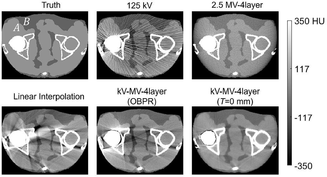
Axial images of the digital pelvis scan simulation, with unilateral titanium hip insert, as obtained from several acquisition and reconstruction techniques. As a reference, the ground truth attenuation image at 65 keV is also shown.

In addition to this qualitative evaluation, contrast and CNR were evaluated from ROIs near the muscle-adipose boundary at points A and B in in Figure 6. It was found that the Hounsfield (HU) difference between muscle and adipose was about 50% greater for the kV-MV proposal than for the 2.5 MV-only image. Likewise, CNR increased with the kV-MV technique from about 3.5 to 7.5.

Results for the digital thorax in Figure 7(a) show similar qualitative characteristics. Standard kV-CBCT, linear interpolation, and kV-MV-OBPR all exhibited dark streaks lancing into the heart from the region of the pedicle screws. Additionally, kV-MV-OBPR produced images with strong residual beam hardening artifacts that obscured most of the vertebra. These artifacts were greatly reduced in the images from MV-only and from the proposed kV-MV method. Residual dark streaks were more noticeable in the kV-MV images as compared to MV-only. However, the kV-MV images were able to better separate the screws from the cortical bone boundaries of the vertebra. This may be due to the more rudimentary beam hardening correction algorithm used by the MV-only reconstruction, which was based on a less detailed, water-equivalent object model than the two-material model used by RPME.

Figure 7:

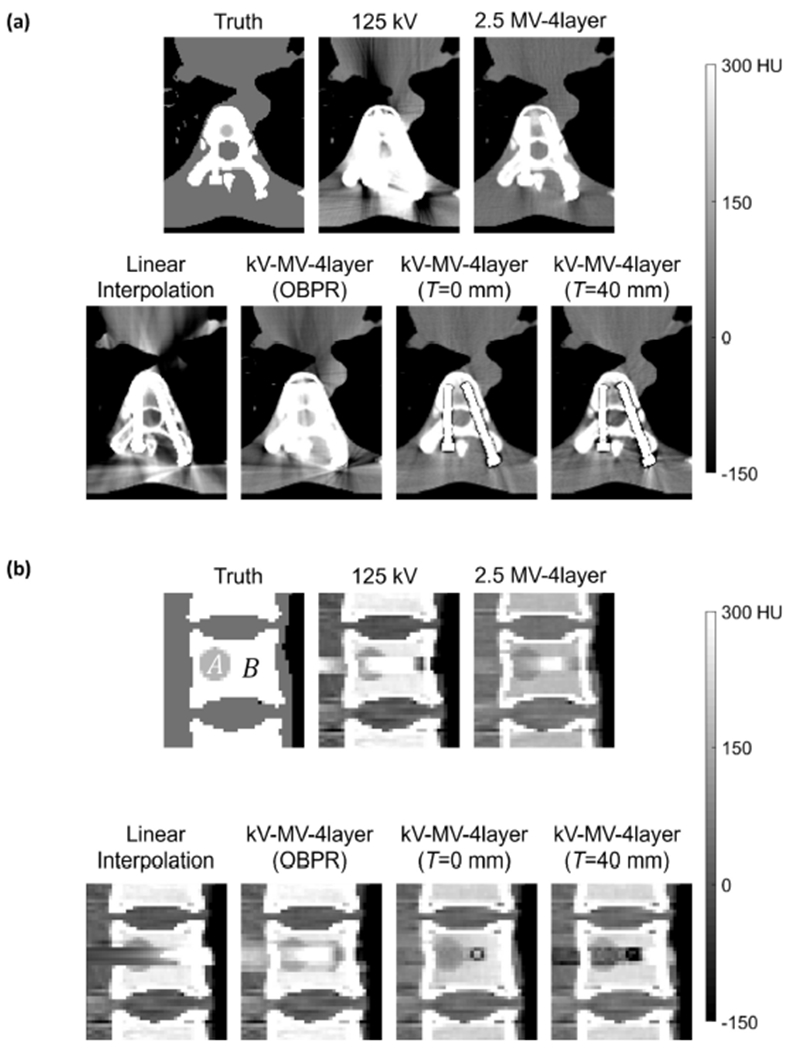
Images of the digital thorax scan simulation, with titanium pedicle screws, as obtained from several acquisition and reconstruction techniques. As a reference, the ground truth attenuation images at 65 keV are also shown. (a) Axial view (b) Sagittal view.

In the sagittal images of Figure 7(b), it is seen that the proposed kV-MV technique increased the HU difference between trabecular bone and lesion tissue, leading to better overall lesion conspicuity than for MV-only. Region of interest measurements between the two regions (marked as A and B in Figure 7(b)) indicated a two-fold increase in the HU difference when basic inpainting $\left(T\text{=}0\mathrm{m}\mathrm{m}\right)$ was used and a three-fold increase with the more selective inpainting $\left(T\text{=}40\mathrm{ }\mathrm{m}\mathrm{m}\right)$.

By excluding kV-CBCT projection rays transecting low metal thicknesses from the overpainting step, it was expected that higher photoelectric interactions would yield higher contrast. This is indeed what is observed in the $T\text{=}40\mathrm{m}\mathrm{m}$ case, although this contrast improvement is non-uniform over the volume of the lesion. Further work on this technique will be needed to extend the effect beyond just the the metal affected voxels in the vertebra.

3.2. Real Phantom Results

Visual and quantitative results for the real phantom scans are presented in Figure 8 for the bi-lateral aluminum insert configuration and in Figure 9 for the unilateral titanium configuration. The trends there generally mirror what was observed in simulation. Namely, the proposed kV-MV method strongly reduces artifact levels from those observed in standard kV-CBCT, but with some compromise in soft-tissue differentation, quantified here in terms of CNR. Indeed, CNR was approximately 30% lower for the kV-MV-4layer technique than for the metal-free kV-CBCT images. As compared to MV-CBCT, however, CNR is significantly improved (about 3-fold) compared to the MV-1layer architecture that is in clinical use.

Figure 8:

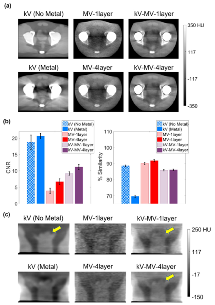
Comparison of different imaging techniques as applied to real pelvis phantom with bilateral aluminum hip inserts. (a) Reconstructed axial slices through femoral heads. (b) Quantifications of contrast-to-noise (CNR) and artifact reduction (% Similarity). Error bars show standard deviations. (c) Reconstructed coronal slices through prostate.

Figure 9:

Comparison of different imaging techniques as applied to real pelvis phantom with unilateral titanium hip insert. (a) Reconstructed axial slices through femoral heads. (b) Quantifications of contrast-to-noise (CNR) and artifact reduction (% Similarity). Error bars show standard deviations. (c) Reconstructed coronal slices through prostate.

Residual artifacts in the kV-MV images are more prominent than were observed in simulation, since here the reconstruction algorithm must contend with physical modeling uncertainties and the presence of residual uncorrected scatter. However, % Similarity is only about 5% lower for kV-MV than for MV-CBCT alone. Overall, delineation of the bladder greatly improved as compared to conventional kV-CBCT and as compared to MV-CBCT from a clinical 1-layer detector architecture.

The impact of the 4-layer MV-detector on kV-MV performance is not as apparent visually in the axial images of Figure 8 and Figure 9 as is the impact on MV-CBCT performance. Since the kV-MV imaging technique receives contributions from both kV- and MV-CBCT data, improvements in the MV detection efficiency alone do not carry as much weight as for MV-CBCT. Also, noise in the kV-MV images is damped by the roughness penalties imposed by RPME.

Nevertheless, the coronal cross-sections through the prostate shown in Figure 8(c) and Figure 9(c) indicate an improvement in the delineation of the upper (superior) sections of the prostate, marked in the figures by arrows.

In Figure 10, the effect of varying the inpainting threshold T on artifact reduction is analyzed. For the aluminum bilateral inserts, it is seen that $\mathrm{T}\text{=}80\mathrm{m}\mathrm{m}$ gave the optimal % Similarity. The parameter choice that we used for Figure 8 results $(\mathrm{T}\text{=}70\mathrm{m}\mathrm{m}$) gave insignificantly different performance from the optimum. The diameter of the spheres was 6.35 mm, so an optimal threshold of $\mathrm{T}\text{=}80\mathrm{m}\mathrm{m}$ basically indicated that only lateral x-ray paths through the phantom, attenuated by both inserts, were worth overpainting. In the other projections, attenuated by only one sphere, kV-CBCT photons were able to penetrate well enough to give healthy measurements. Conversely, for the unilateral titanium case, Figure 10(b) shows that any $\mathrm{T}\text{<=}50\mathrm{m}\mathrm{m}$ was optimal, which corresponded to overpainting in all projection views. In other words, because of the higher attenuating titanium composition of the sphere, as compared to aluminum, it became necessary to overpaint all metal-affected pixels to achieve optimal artifact reduction. Recall that we chose $\mathrm{T}\text{=}0\mathrm{ }\mathrm{m}\mathrm{m}$ for the experiments of Figure 9, and so we see that this was in the optimal range.

Figure 10:

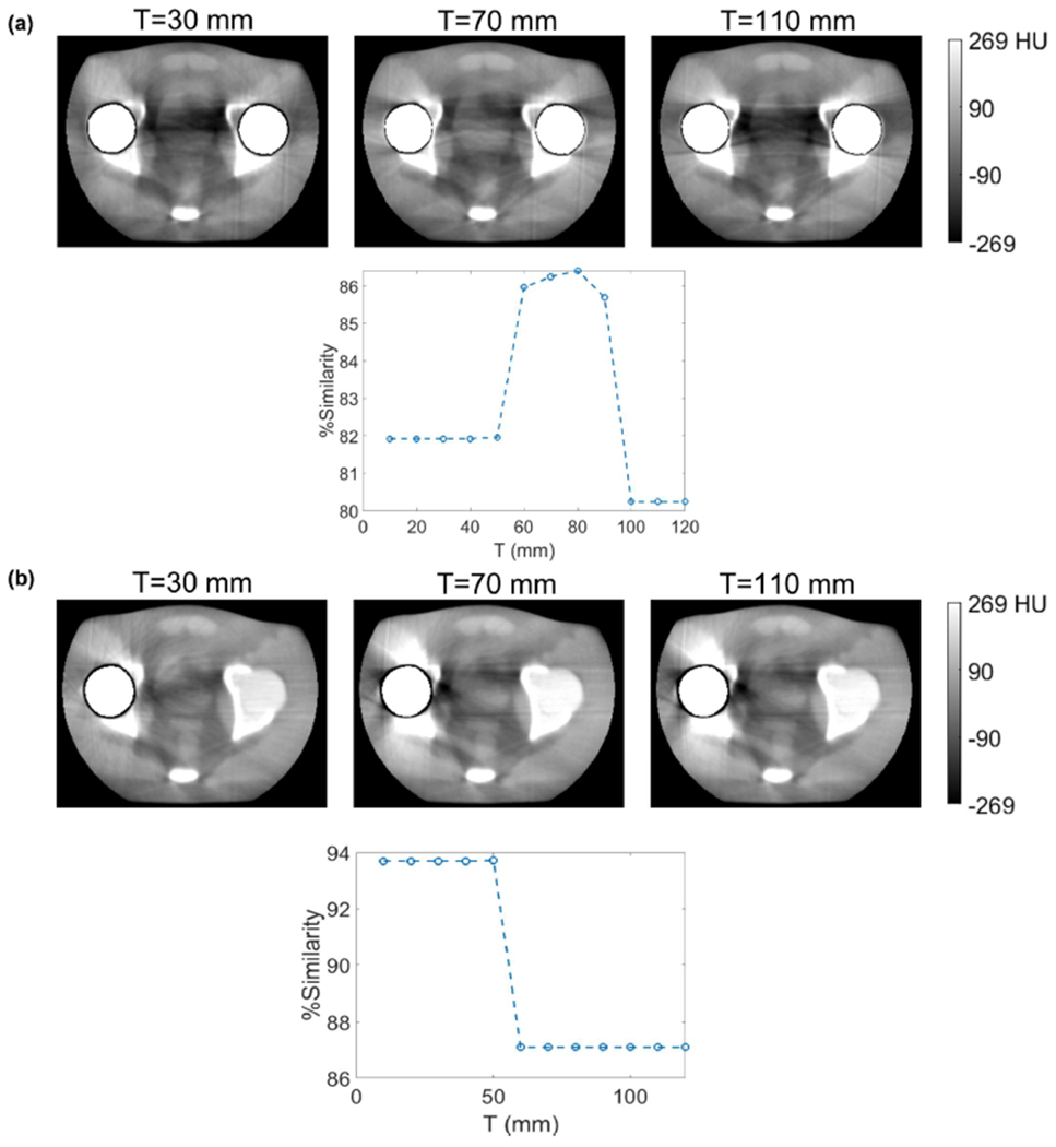
Influence of inpainting threshold parameter, T, on artifact reduction performance. (a) Bi-lateral aluminum inserts. (b) Unilateral titanium inserts

4. Conclusions and Discussion

A method has been proposed that combines concurrently acquired, on-treatment kV-CBCT and MV-CBCT data to achieve artifact-reduced 3D images for radiotherapy guidance. A distinguishing feature of the method is a preliminary MV-CBCT reconstruction to determine the 3D position and pose of metal implants. This prior analysis allows one to construct detailed poly-energetic models of photon transport through the metal, and to generate inpainting data while avoiding the needed for dynamic source collimation. Additionally, by pre-calculating metal thicknesses seen by each measured projection pixel, our method anticipates which measurements will be most significantly photon-starved. This, in turn, allows the algorithm to overpaint metal-affected kV-CBCT pixels more selectively, leading to better optimized visibility in some regions of the reconstructed volume.

The use of MV-CBCT at low dose settings suitable for on-treatment 3D imaging meant that images would be noiseprone. The approach in this paper addressed this in part through hardware, specifically the use of a 4-layer, high DQE MV-detector and a 2.5 MVp beam, to improve x-ray detection efficiency. In part also, it used a noise-reduced beam hardening correction algorithm called RPME, which diminishes noise using edge-preserving Huber roughness penalties.

The proposed kV-MV technique was tested in both simulated and real phantom experiments, and compared to more basic imaging techniques, including MV-CBCT using the Halcyon’s single-layer detector architecture and to clinically conventional kV-CBCT. The kV-MV-CBCT method was found to achieve, at matched edge blur, a trade-off in CNR and artifact suppression giving better delineation of critical soft tissue boundaries in the spine, bladder, and prostate. In the real phantom experiments, CNR improvements over 1-layer MV-CBCT by a factor of 3 were observed.

Our real data experiments focused on a pelvis phantom emulating aluminum and titanium hip replacements, which are the two most common materials in such prosthetics. The diameters of the femoral head replacements were 2.5”, which is at the upper end of the size range seen in actual hip replacement procedures, and thus presented maximal challenge for the imaging techniques. The experiments presented in the paper considered two hip implant configurations, namely bilateral aluminum implants and a unilateral titanium implant. We also tested unilateral aluminum and bilateral titanium configurations, but these were not presented in the paper. The unilateral aluminum configuration did not sufficiently challenge conventional kV-CBCT to be of much interest. Conversely, bilateral titanium induced too much photon starvation to image even in MV-CBCT, or at least at the 2.5 MV energy levels tested here. Although our kV-MV method allows for the kV-imager measurements to be photon-starved, it is confounded if the MV-imager measurements are starved as well. Potentially, moving to 6 MV LINAC energies could address this case. However, the Varian Edge system lacks the capability to acquire 6 MV CBCT data at below 52 MU, so we were unable to do such experiments at realistic dose levels. In future work, we may experiment with Varian’s Ethos LINAC, which does allow 6 MV CBCT at lower exposures, but there are logistic and regulatory issues to be addressed before the multi-layer imager can be installed on such a system.

An additional area for future work will be in the area of scatter correction. More pronounced residual artifacts were observed in real data experiments than with digital phantoms. This was likely due to interference from residual scatter. It is possible that newer scatter correction methods may improve on the fASKS scatter removal method used in this paper and so better realize the performance potential of the kV-MV technique.

REFERENCES

- Faddegon BA et al. 2008. Low dose megavoltage cone beam computed tomography with an unflattened 4 MV beam from a carbon target Med. Phys 35 5777–86 Online: http://doi.wiley.com/10.1118/1.3013571 [DOI] [PubMed] [Google Scholar]
- Feldkamp LA et al. 1984. Practical cone beam algorithm J. Opt. Soc. Am. A 1 612–9 [Google Scholar]
- Jacobson MW et al. 2021. Abbreviated on-treatment CBCT using roughness penalized mono-energization of kV-MV data and a multi-layer MV imager Phys. Med. Biol 66 135001 Online: https://iopscience.iop.org/article/10.1088/1361-6560/abddd2 [DOI] [PMC free article] [PubMed] [Google Scholar]
- Joseph PM and Spital RD 1978. A Method for Correcting Bone Induced Artifacts in Computed Tomography Scanners J. Comput. Assist. Tomogr 2 100–8 [DOI] [PubMed] [Google Scholar]
- Kalender WA et al. 1987. Reduction of CT artifacts caused by metallic implants Radiology 164 576–7 [DOI] [PubMed] [Google Scholar]
- Lindsay C et al. 2019. Investigation of combined kV/MV CBCT imaging with a high-DQE MV detector Med. Phys 46 563–75 Online: http://doi.wiley.com/10.1002/mp.13291 [DOI] [PMC free article] [PubMed] [Google Scholar]
- Rinkel J et al. 2008. Computed tomographic metal artifact reduction for the detection and quantitation of small features near large metallic implants: A comparison of published methods J. Comput. Assist. Tomogr 32 621–9 Online: https://journals.lww.com/jcat/Fulltext/2008/07000/Computed_Tomographic_Metal_Artifact_Reduction_for.22.aspx [DOI] [PubMed] [Google Scholar]
- La Rivière P J 2005. Penalized-likelihood sinogram smoothing for low-dose CT Med. Phys 32 1676–83 Online: http://doi.wiley.com/10.1118/1.1915015 [DOI] [PubMed] [Google Scholar]
- La Rivière P J et al. 2006. Penalized-likelihood sinogram restoration for computed tomography IEEE Trans. Med. Imag 25 1022–36 [DOI] [PubMed] [Google Scholar]
- La Rivière P J and Pan X 2000. Nonparametric regression sinogram smoothing using a roughness-penalized Poisson likelihood objective function IEEE Trans. Med. Imag 19 773–86 [DOI] [PubMed] [Google Scholar]
- Stayman JW et al. 2012a. Model-Based Tomographic Reconstruction of Objects Containing Known Components IEEE Trans. Med. Imaging 31 1837–48 Online: http://www.ncbi.nlm.nih.gov/pubmed/22614574 [DOI] [PMC free article] [PubMed] [Google Scholar]
- Stayman JW et al. 2012b. Model-based reconstruction of objects with inexactly known components Proceedings of SPIE--the International Society for Optical Engineering vol 8313, ed Pelc NJ et al. p 83131S Online: http://www.ncbi.nlm.nih.gov/pubmed/26203201 [DOI] [PMC free article] [PubMed] [Google Scholar]
- Sun M and Star-Lack JM 2010. Improved scatter correction using adaptive scatter kernel superposition Phys. Med. Biol 55 6695–720 [DOI] [PubMed] [Google Scholar]
- Tang G et al. 2016. Low-dose 2.5 MV cone-beam computed tomography with thick CsI flat-panel imager J. Appl. Clin. Med. Phys 17 235–45 Online: http://doi.wiley.com/10.1120/jacmp.v17i4.6185 [DOI] [PMC free article] [PubMed] [Google Scholar]
- Uneri A et al. 2019. Known-component metal artifact reduction (KC-MAR) for cone-beam CT Phys. Med. Biol 64 Online: https://pubmed.ncbi.nlm.nih.gov/31287092/ [DOI] [PMC free article] [PubMed] [Google Scholar]
- Wu M et al. 2014. Metal artifact correction for x-ray computed tomography using kV and selective MV imaging Med. Phys 41 121910 Online: http://doi.wiley.com/10.1118/1.4901551 [DOI] [PMC free article] [PubMed] [Google Scholar]
- Xu S et al. 2017. Polyenergetic known-component CT reconstruction with unknown material compositions and unknown x-ray spectra Phys. Med. Biol 62 3352–74 Online: http://www.ncbi.nlm.nih.gov/pubmed/28230539 [DOI] [PMC free article] [PubMed] [Google Scholar]
- Yazdia M et al. 2005. An adaptive approach to metal artifact reduction in helical computed tomography for radiation therapy treatment planning: Experimental and clinical studies Int. J. Radiat. Oncol 62 1224–31 [DOI] [PubMed] [Google Scholar]
- Yin F-F et al. 2005. A technique for on-board CT reconstruction using both kilovoltage and megavoltage beam projections for 3D treatment verification Med. Phys 32 2819–26 [DOI] [PubMed] [Google Scholar]
- Zhang C et al. 2017. Polyenergetic known-component reconstruction without prior shape models ed T G Flohr et al (SPIE) p 101320O Online: http://proceedings.spiedigitallibrary.org/proceeding.aspx?doi=10.1117/12.2255542 [DOI] [PMC free article] [PubMed]