Circuital modelling in muscle tissue impedance measurements

Abstract

Electrical impedance spectroscopy (EIS) stands as a widely employed characterization technique for studying muscular tissue in both physio/pathological conditions. This methodology commonly involves modeling tissues through equivalent electrical circuits, facilitating a correlation between electrical parameters and physiological properties. Within existing literature, diverse equivalent electrical circuits have been proposed, varying in complexity and fitting properties. However, to date, none have definitively proven to be the most suiTable for tissue impedance measurements. This study aims to outline a systematic methodology for EIS measurements and to compare the performances of three widely used electrical circuits in characterizing both physiological and pathological muscle tissue conditions. Results highlight that, for optimal fitting with electrical parameters relevant to tissue characterization, the choice of the circuit to be fitted closely hinges on the specific measurement objectives, including measurement parameters and associated physiological features. Naturally, this necessitates a balance between simplicity and fitting accuracy.

Highlights

• •A systematic measurement procedure has to be followed and shared in applying EIS.
• •Changes in equivalent electrical parameters can depend on the employed circuit.
• •The “Cole-Cole Circuit” is a good trade-off, between performances and error size.

1. Introduction

Electrical impedance spectroscopy (EIS) is an important, widely used, non-destructive, characterization technique employed in many applications (i.e., for characterizing corrosion phenomenon, the performances of the fuel cells, or any other electrochemical process) [[1], [2], [3], [4]]. The distinctive characteristic of the technique is that it focuses on the analysis of passive characteristics of the material. The living tissues also provide some impedance to the passage of electric current so that EIS has been employed on human body as a diagnostic tool to be used in different fields. To characterise muscular tissue, EIS has been employed for studying different physiological and pathological conditions [[5], [6], [7], [8], [9]], effects of age [10,11], and for characterising muscle changes during a fatigue state [12].

In EIS [13], as well as in several others research fields, it is common to model systems by means of equivalent electrical circuits which provide a simplified description of the properties of the measured materials or organs [[13], [14], [15], [16]]. In addition, it is widely accepted that an appropriate choice of the equivalent circuit and a good compromise between several aspects (i.e., parameters, level of complexity) are fundamental for a good fitting [17,18]. This is true also for EIS applications in muscle tissue analysis [7,8]; indeed, there are studies concerning changes in the electrical properties of muscular tissue at low levels of contraction or testing health condition of muscles in elderly subjects [6,9,19].

As this approach considers a correlation between circuit components and physiological elements, an appropriate choice of the model is necessary in order to highlight, by means of the circuit elements, the underlying physical and physiological processes [14]. Indeed, in literature, different equivalent electrical circuits have been proposed [5,8,13,16,20] and changes in the values of models’ parameters, or some combination of them, are related to biological characteristics. The authors agree with this consideration and hypotise a physiological meaning for some electrical parameters, so that they expect a change of their values under different physiological conditions (as for each biological parameter). In particular, a significant change is expected for those electrical parameters more strictly related to physiological characteristics.

Nevertheless, it is worth underlying that, until today, none of the most employed electrical circuits has definitely proved to be the most effective for muscular tissue characterisation through electrical parameters.

Besides, a systematic description of the procedure to be employed in EIS muscular measurements is lacking in literature; a methodology to follow, with particular emphasis to the circuit choice step, is here proposed and described.

Encouraged by the scientific literature in this research field [7,8], and by the different significant studies on this topic [1,[12], [13], [14]], the aim of this paper is twofold: (i) to describe a systematic procedure of EIS of muscular tissue, (ii) to evaluate the performances of three electrical circuits, generally employed for the characterisation of the muscular tissue in different physiological conditions, that have been compared with respect to sensitivity of their parameters and to fitting errors. The first objective aims to identify a shared procedure in EIS measurements. The second objective faces the problem of assessing the electrical circuits’ effectiveness.

2. Methods and materials

2.1. Background

In bioimpedance measurements, to highlight the correlation between physiological changes of a system under analysis and the impedance value of the system itself [13,14], systems’ models (or electrical models) are employed. In particular, from the literature, it is known that it is possible to model the bioimpedance behavior through equivalent electrical circuits. Nowadays, this methodology has become among the main EIS data analysis methods [13,21,22]. This is due also to the capability of modeling nonlinear phenomena, related to inhomogeneities in the tissues and to the presence of a distribution of relaxation times, by introducing non real circuit elements. Nevertheless, a systematic methodology, shared and accepted, is still lacking.

2.2. Measurement and methodology

Based on the literature [8] regarding tissue impedance measurements, a specific and more detailed methodology is proposed, schematically represented in Fig. 1.

Fig. 1.

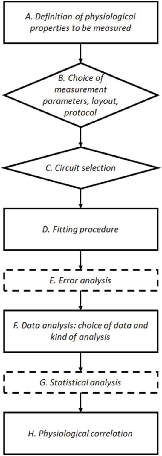
Scheme of the procedure to be employed for EIS measurements. With dotted contours, non-core steps. In diamonds, the steps for which an operator decision is required.

In the following, each step will be described, and particular attention will be devoted on step C, which is the main focus of this paper.

Before describing the different steps of the procedure shown in Fig. 1, it is important to highlight that some steps (i.e., E: “Error analysis” and G: “Statistical analysis”) are introduced in order to improve and complete the comprehension of the phenomenon under analysis; as well as usually done in signals processing. At the same time, it is important to underline that the steps “Choice of measurement parameters” (B), “Circuit selection” (C), “Fitting procedure” (D) and “Data analysis: choice of data and kind of analysis” (F) require specific and very critical decisions by the operator.

From the methodological point of view, the first step, “Definition of physiological properties to be measured” (step A in Fig. 1), often implies the choice of the measurement type. For example, both EMG and EIS methodologies study muscle properties and physiological behaviours, but EMG focuses on active neuro-muscular electrical activity whereas EIS analyses muscle passive electrical characteristics [20].

In EIS measurements, when the physiological properties to be analysed (for example, inherent electrical activity, biochemical or bioimpedance changes, tissue relaxation frequencies [5,8,20,21], and hence the kind of measurement have been chosen, it is necessary to fix all the related parameters (step “Choice of measurement parameters” - B - in Fig. 1). Some of them (such as the frequency range for EIS) have to be chosen considering the physiology of the system under analysis, other depend on its morphology (for example, electrodes positioning), others are important since can affect measurement results (for example, current value, number of trials, etc.). However, their values have to be always carefully set, based on the nature of the tissue and the physiological phenomena to be measured.

In EIS applications, electrical impedance can be measured as the ratio between voltage and current; to this aim, an alternating current is injected via surface electrodes and the resulting voltage drop over a selected tissue or muscle group is measured [8,12,20]. The value of the current intensity has to comply with safety levels and the voltage drop has to be kept constant over the portion of tissue under study. The impedance is normally measured using a small excitation signal, so that the response is pseudo-linear. The chosen frequency range elicits different components and frequency dependent phenomena of muscular tissue [21]. Besides, different regions of frequency response can be defined, each of them due to different passive properties such as conductivity and permittivity [21]. Furthermore, electrodes layout and protocol can determine incorrect and/or not comparable results [7].

Obviously, even if measurement parameters and set-up are fixed, different equivalent electrical circuits can be employed. Equivalent electrical circuits allow to physiologically and clinically interpret tissue's changes. Indeed, the characterization of the tissues can be based on the knowledge of their electrical properties in the frequency spectrum [13]. As clearly stated in Ref. [14], “such circuits are only models that help in understanding the behaviour of those tissues from an electrical point of view”; indeed, biological tissues show a very complex and frequency dependent behaviour, difficult to completely explain by means of relatively simple circuit elements. Despite to this difficulty, it has been demonstrated that by observing the variations of some electrical parameters different human tissue types can be characterized [21]. This is the reason for that, as mentioned, choosing the most appropriate model is a key step in impedance measurements (step “Circuit selection” - C - in Fig. 1) and, here, this issue is dealt with particular attention. Elsewhere [6,7], steps “Definition of physiological properties to be measured” (A), “Choice of measurement parameters” (B), “Fitting procedure” (D) and “Data analysis: choice of data and kind of analysis” (F) are dealt in detail; so that here we focused on the other steps.

The choice of the fitting procedure (step “Fitting procedure” - D - of Fig. 1) refers to the known issue of the fitting procedure, on which the performances of EIS measurements are largely dependent on. Despite to its importance, the employed procedure is often not cited, non-linear fittings based on square error minimization are generally used [1].

Important information concerning the reliability of the chosen model can be obtained by the “Error analysis” (step E in Fig. 1); however, as mentioned, this analysis is very often not available in literature, even in valuable studies [11,16].

After measurements execution, when all impedance data are available, from the methodological point of view, the kind of data processing, in case also the statistical analysis, and the kind of results presentation have to be chosen (steps “Data analysis: choice of data and kind of analysis” - F - and “; Statistical analysis”; - G - in Fig. 1).

Finally, for future practice, clinical applications, the physiological interpretation of the obtained results has to be carried out (step “Physiological correlation” - H - in Fig. 1), in order to get the correlation between physiological phenomena and electrical components, which is a not easy topic, since tissues show a rather complex behavior.

2.3. Impedance data

Following the procedure described in the previous section, EIS methodology has been employed for studying physiological changes in muscle tissue under different conditions. In particular, a database of impedance measurements was realised and employed for the current work. For impedance recordings, sixteen healthy volunteers (11 men and 5 women, age 27.5 ± 7.1), not affected by any neurological or musculoskeletal disorder, were involved in the measurements.

The measurement procedure, instrumentation and measurement set-up are based on the literature [6,23], where all details are reported. Essentially, all they concern the step “Choice of measurement parameters, lay out and protocol” (B) [8] of the scheme shown in Fig. 1. Summarizing, EIS measurements were carried out by employing tetrapolar measurements on the forearm flexor muscles; each test involved three trials, i.e., impedance measurement of the muscle tissue, corresponding to different conditions: muscle at rest, muscle contraction and 4 min after the contraction. The impedance of the tissue under analysis was evaluated as ratio between the acquired sinusoidal voltage and the injected current signal; the voltage across the measured tissue was set to 20 mV. The frequency range was 1–60 kHz, according to further works [[6], [7], [8]]; so that the EMG surface signal was deleted and part of the β region (10³–10⁷ Hz [20,21]) was elicited, in this frequency's region 11 out of 12 human tissue elements are elicited [[6], [7], [8],20,21,[24], [25], [26]]. The linear frequency sweep was of 10 points. For each frequency the impedance was calculated as mean over five measurements. Therefore, each trial lasted about 1 min and a whole test about 7 min. The electrodes were posed in line on the forearm, the current electrodes were placed on the elbow and the wrist and the voltage ones between them with an inter-distance of 6 cm, starting from 3 cm distance by the antecubital fossa. All subjects sat relaxed with the arm on a desk keeping their hand flat on the desk, in line with the forearm and with the palm turned upward. As said, each subject underwent to a test protocol consisting of three trials: i) rest condition (steady state); ii) sustained isometric contraction (60–70% of the maximum effort); iii) 4 min after contraction. The prototyped proof demonstrator was based on a battery powered notebook PC implemented with an AD/DA board and an analog interface; and the software, developed in LabVIEW for impedance evaluation, provides average modulus and phase of five measurements executed for each frequency value.

2.4. Equivalent electrical circuits

For the characterisation of the muscular tissue, and in particular for the analysis of their physiological properties, an electrical modelling is often employed by means of equivalent electrical circuits [13,21]. Indeed, these circuits represent important models, since each circuit element has a physiological meaning; for example, resistors represent current flows through intra and extracellular fluids, and capacitors represent membrane behavior [5].

For this work, the performances of three different electrical circuits, largely used in literature and in clinical applications, are compared. The circuits #1, #2, #3 are named according to their main proposer. Let us remember that #1 and #2 [5,16] have been successfully used to characterise pathological muscle conditions, whereas #3 introduces non-linear elements resulted very useful in EIS modelling [[12], [13], [14]]. For each circuit are here reported the impedance formula and, in case, the equivalent physiological significance of each component.

2.4.1. Circuit #1: Rutkove-Ching

Circuit # 1 is the simplest circuit, which involves three elements corresponding to the main physiological constituents of the cell. It has been successfully employed from Rutkove and Ching [11,16] to study age-dependent changes in muscular tissue or patients with acute lower back pain and it is shown in Fig. 2.

Fig. 2.

Electrical circuit here called “Circuit #1: Rutkove-Ching”. In this circuit, R₀ is the extracellular resistance [13], R_iis intracellular resistance [20] and C_mis the membrane capacitance.

The tissue impedance computed by means of the “Circuit #1: Rutkove-Ching” results equal to (Eq. (1) and Eq. (2)):

$$Z_{tissue}=\frac{\left(R_i+X_C\right){*R}_0}{R_i+R_0+X_C}$$ (1)

$$\text{where}:X_C=\frac{1}{j\omega C_m}$$ (2)

2.4.2. Circuit #2: Shiffman

Then, a circuit with five parameters has been analysed; this circuit, shown in Fig. 3, has been used from Shiffman et al. [5] in order to also take into account some intracellular organelles. It has been employed, for example, in characterizing muscle in neuromuscular disease or during clinical drug testing.

Fig. 3.

Electrical circuit here called “Circuit #2: Shiffman”. In this circuit, R₀, R_i and C_m are again extracellular resistance, intracellular resistance, and membrane capacitance, respectively. Then, R_or and C_or are resistance and capacitance associated with intracellular organelles [5].

In this case, for the tissue impedance estimation, the following formula has to be employed (Eq. (3) and Eq. (4)):

$$Z_{tissue}=\frac{\left(Z_i+X_C\right)*R_0}{Z_i+{R_0+X}_C}$$ (3)

$$\text{where}{Z}_i=\frac{Z_{or}*R_i}{Z_{or}+R_i}\text{and}{Z}_{or}=R_{or}+\frac{1}{j\omega C_{or}}$$ (4)

2.4.3. Circuit #3: Cole-Cole

Finally, the performances of the circuit proposed by Cole and Cole, and already employed in literature [8,13,14], for example for verifying electrical parameters’ sensitivity in different muscular conditions, has been studied.

With respect to the others, the main difference of this circuit, shown in Fig. 4, is the introduction of a pseudo-capacitor, the ‘‘constant phase element’’ (CPE), i.e., a further impedance called Z_cpe [13,14] that produces a phase shift nearly constant, useful, and accepted elsewhere [13,14,26,27] to fit EIS data, in biological tissues measurements too.

Fig. 4.

Electrical circuit here called “Circuit #3: Cole-Cole”. In this circuit, R₀ is the extracellular resistance, R_∞ represents the tissue resistance at high frequency and Z_cpe is the impedance due to the constant phase element [13].

The CPE has the following analytical expression (Eq. (5)) [14]:

$$Z_{CPE}=A{\left(j\omega \right)}^{-\delta }$$ (5)

where ω=2πf, (f is the frequency), A is a constant, and represents the amplitude of the impedance pseudo-capacitive, and δ (0 ≤ δ ≤ 1) is a dimensionless empirical parameter characteristic of the distribution of the relaxation times of the various structures forming the tissue [8].

From this circuit, the tissue impedance can be computed as (Eq. (6)):

$$Z_{tissue}=R_{\infty }+\frac{R_0-R_{\infty }}{1+{\left(j\omega T\right)}^{\delta }}$$ (6)

where T is the circuit time constant and is in the following relationship (Eq. (7)) with the parameter A:

$$A=\left(R_0-R_{\infty }\right)\frac{1}{T^{\delta }}$$ (7)

By using the “Circuit #3: Cole-Cole”, the tissue under examination can be characterized through 5 direct parameters (R_ω, R₀, R₀ - R_∞, δ, T) to be correlated to biological components [8].

It is worth highlighting that, at very-high and very-low frequencies, biological tissues are commonly represented as pure resistors so that, in all the circuits, the impedances can be replaced by the ideal resistors. Besides, R₀ represents the tissue resistance at low frequencies.

In Table 1 the parameters involved in the different electrical circuit models are summarised, and, in case, their equivalent physiological significance are reported.

Table 1.

circuit models and involved electrical parameters [5,13,20]. Let us remember that Circuit #1 is Rutkove-Ching, Circuit #2 is Shiffman and Circuit #3 is Cole.

Electrical parameter	Circuit in which it is present	Meaning
R0	#1, #2, #3	Extracellular resistance
Ri	#1, #2	Intracellular resistance
Cm	#1, #2	Membrane capacitance
Ror	#2	Resistance of intracellular organelles
Cor	#2	Capacitance of intracellular organelles
R∞	#3	Parallel between internal and external resistance
T	#3	Circuit time constant
δ	#3	Distribution of relaxation times

2.5. Data analysis

About the step “Fitting procedure” (D), for fitting experimental data to the circuits, among the most common procedures employed in literature and in commercial instrumentations, as already done in other literature studies, the LMS using LEVM software [7,8,28] has been employed. It is based on the complex nonlinear least squares fit method, since it is simple to use, explained in detail and broadly employed both for industrial and scientific application of EIS.

In this way, the values of all parameters (C_m, R₀, R_i, C_or, R_or, R_∞, R₀ - R_∞, δ, T, A) of the three equivalent electrical models considered, and the values of R₀ (for its link to the extra-cellular resistance [14,16]), for each of the three trials mentioned in section 2.2, were estimated.

In this study, in order to establish which electrical circuit can be the most suiTable, the error analysis becomes a key step; indeed, as mentioned, this error represents the reliability of the model in fitting the experimental data. Therefore, the changes in electrical parameters’ values and the error obtained in matching experimental data have been studied. To this aim, the fitting error (step “Error analysis” – E) has been computed. It is provided by the software, as an output parameter, in order to estimate the best correspondence between experimental data and theoretical model.

After outliers deleting, according a procedure reported in literature [8], the steady state was considered as a reference and for the other conditions (contraction and 4 min after) the relative variations of all electrical parameters were evaluated.

A t-test was adopted to verify the statistical significance of the obtained results. The test was considered significant if it was p ≤ 0.05 and was carried out also considering the comparison between the state of muscle contraction and that 4 min after contraction.

3. Results

As mentioned in section 2.3. “Impedance data”, and published in Ref. [8], the capability of the different electrical elements to characterise some muscle physiological conditions has been tested. In particular, rest, contraction and muscular state some minutes after contraction were considered for the study.

The step “Data analysis: choice of data and kind of presentation” (F) of the scheme of Fig. 1 can be very important to simplify the following data physiological interpretation (step “Physiological correlation” – H). It is known that a high variability affects biomedical measurements, so that, according to Refs. [7,8], relative measurements have been employed, rather than absolute measurements, to reduce this variability. The initial rest state (let us call RS) of the muscle under analysis was chosen as reference steady state, and values of the electrical parameters obtained during the muscle contraction (here named CN) and 4 min (simply 4 in the following) after contraction were computed as relative variations; hence, obtained results were labelled as CN\RS, relative variations of the different parameters concerning the contraction state with respect to the reference steady state and 4\RS, relative variations of the values obtained 4 min after the contraction with respect to the steady state; RS\RS refers to the reference steady state, i.e. null values.

In Table 2 above shown, the results of the statistical analysis concerning all the parameters of the three analysed circuits are reported.

Table 2.

p-values of the t-test. In bold statistically significant results. Let us remember that Circuit #1 is Rutkove-Ching, Circuit #2 is Shiffman and Circuit #3 is Cole-Cole. Moreover, X/RS labels the relative variation of the parameter computed in the state X with respect to the state RS; 4/CN: 4 min after contraction with respect to contraction.

		CN/RS	4/RS	4/CN
Circuit #1	R0	0.3245	0.0004	0.3245
	Ri	0.0462	0.5391	0.0831
	Cm	0.3245	0.3246	0.3246
Circuit #2	R0	0.0000	0.0060	0.0000
	Ri	0.3452	0.0404	0.0916
	Cm	0.4656	0.4803	0.1559
	Ror	0.4656	0.4803	0.1559
	Cor	0.4718	0.0364	0.2237
Circuit #3	R0	0.0000	0.0008	0.0000
	R∞	0.0098	0.6334	0.1172
	R0 - R∞	0.5929	0.0555	0.0298
	T	0.0002	0.1306	0.0020
	δ	0.4067	0.1006	0.5031

From data shown in Tables 2 and it is possible to observe that, globally, as expected, R₀ is the electrical parameter most sensible to muscle status variations (due to its strict correlation with the extra-cellular fluid). Its changes, indeed, are statistically significant if circuits #2: Shiffman and # 3: Cole-Cole are employed, whereas, with the circuit #1, only in the state 4 min after contraction it is significant.

R_i shows a different behavior in the different schemes. With respect to the RS, it decreases significantly in the CN, and slightly increases in the state 4 min after contraction, if the “Circuit #1: Rutkove-Ching” is used; but the decrease is lesser in the contraction state, and the increase is significant 4 min later, if the “Circuit # 2: Shiffman” is used.

Other parameters show statistically significant variations only in specific cases (for example, C_or, “Circuit #2: Shiffman”, in condition 4/RS; R_∞, “Circuit #3: Cole-Cole”, in the condition CN/RS); and some of them have no direct and simple physiological interpretation (like T, circuit time constant).

Summarizing, 2/9 values, i.e., just over 20%, are statistically significant when “Circuit #1: Rutkove-Ching” is employed; just over 30%, 5/15 values, are statistically significant when “Circuit #2: Shiffman” is employed; and almost 50%, indeed 7/15, when “Circuit #3: Cole-Cole” is employed. Therefore, by considering all the parameters, it is possible to observe a higher sensitivity of this circuit.

In Fig. 5 results of the mean fitting errors are reported. The error is a software output which represents the average of the absolute values of the standard deviations, provided in order to make easier the comparison among different fittings. It is very important to highlight that the fitting errors are different for all the muscle states here considered: relaxation, high contraction, 4 min after contraction.

Fig. 5.

Mean values and dispersions of the fitting errors obtained with the three electrical circuits here analysed.

Finally, for sake of completeness, in Fig. 6 the boxplots which shows the errors values obtained across all the participants are reported for each analysed electrical circuit.

Fig. 6.

Boxplots of the errors for each experimental condition (Rest, Contraction, 4-min after contraction) for the three different models: (a) Shiffman circuital model; (b) Rutkove-Ching circuital model; (c) Cole-Cole circuital model.

Let us briefly remember that box plots are useful since they provide a quick visual summary of the distribution of values in a dataset. From the top to the bottom, the horizontal lines represent maximum value, upper quartile, median value, lower quartile, and minimum value, so that in the box there is the most amount of data. Circles identify outliers, which can reveal mistakes or unusual occurrences in data. It is important to underline that it is not an error to also show outliers; in fact, in an in-depth phase, they can help in the detection of errors’ causes.

4. Discussion and conclusion

EIS measurements are gaining increasing interest in the analysis of biological tissues, since they represent a painless, low-cost methodology for tissue characterization. Recently, this technique has been employed even to study the effect on potato tissue of some treatments [29,30]. Many applications concern human tissue, and, in particular, muscle analysis, nowadays an important topic for the scientific community [[30], [31], [32], [33]].

Very often, electrical models, which implement equivalent electrical circuits, are employed for this kind of studies. Indeed, through the changes obtained for the circuit elements’ values, when measuring impedance data, it is possible to know some physiological changes of the tissue. However, there exist multiple proposed electrical circuits, with a different number of electrical components, or involving the same electrical components but in different configurations [5,13,16,29,30].

Furthermore, the results reported in literature are not always in agreement; the reasons can be different. For example, the changes in impedance values reflect a series of different effects, such as the modifications in muscle geometry and/or in metabolic processes; then, the effects of skin, subcutaneous adipose tissue, and bone, as well as the electrodes’ arrangement, can affect the surface measurements [12,34]. Considering this scenario, it is crucial to establish the basic steps of a measurement procedure to be followed and shared. Indeed, a common procedure would allow the comparison of the results obtained from different research groups and the decrease of some variability sources.

With this in mind, the choice of the most suiTable model is a key point in EIS applications. In fact, it is important reminding that the choice of the circuit depends on different conditions, such as, for example, the measurement layout and, in particular, the frequency range. The study in Ref. [21] affirms that, in different frequency ranges, different tissue elements are elicited; so, if the stimulus has a frequency that does not determine a “bioelement” response, the corresponding electrical component is useless and can be eliminated from the electrical scheme.

Hence, in this work, after the presentation of a methodological procedure, proposed for EIS measurements, in order to determine the most suiTable circuit, the performances of the more largely used equivalent electrical circuits have been compared. In particular: the “Circuit #1: Rutkove-Ching”, the simplest one with only three elements; the “Circuit #2: Shiffman”, with five elements, since also involves the analysis of intracellular organelle and the “Circuit #3: Cole-Cole”, with four direct parameters and the fifth indirect were considered for the study.

Before discussing the results obtained, it is important to highlight some important aspects of this work. To the best of our knowledge, this is the first time that a procedure to be followed in EIS measurements has been explicitly and accurately defined. Furthermore, in the literature, there are not many works that rigorously compare the most used electrical circuits. Finally, the fitting error is very rarely considered, it, vice versa, is very important for establishing the reliability of a circuit and its use. Concerning the results, values obtained for the electrical parameters firstly confirm that results can be in disagreement; for example, the behavior of R₀ seems not to be the same, in dependence on the employed circuit.

It is important to put in evidence that aim of this work is not to explain these differences, which will be deepened, rather to evaluate if it is possible to reach a trade-off between the capability to react to physiological changes and the circuit complexity, identified as number of electrical parameters and their connections, which, in turn, determine the circuit impedance. Furthermore, despite the recognized and assessed usefulness of certain models, shared and absolute findings have not been gotten yet. Indeed, above mentioned studies propose the use of another electrical circuit, even in different versions [29,30]. Finally, at the best of the authors’ knowledge, in this study the performances of different models under the same experimental conditions have been compared for the first time.

Comparing the sensitivity of the parameters in the three circuits, i.e., their capability to distinguish the different states (see the results of the t-test reported in Table 2) and the fitting errors, it is possible to observe that the “Circuit #2: Shiffman” shows the worst performances in terms of errors, in opposition to literature's results. Very probably, this is since this circuit is not adequate to experiments carried out in Refs. [7,8], in which there is no interest in organelles reactions; this is a proof of the necessity of properly choosing the adequate model. Indeed, “Circuit #1: Rutkove-Ching”, which is very simple, has performed very well in describing macroscopic clinical phenomena [16]; whereas “Circuit #3: Cole-Cole”, which, in terms of error, did not perform very well, provided very good results in situations which involve also intracellular structures [5,6].

The future work will consist in enlarging the dataset, and in the definition of a procedure/formula for obtaining a correlation between circuit's complexity and error's value. Now, in fact, the relatively small number of measures and the lack of this formula represent the limitations of the study.

However, in order to get a conclusion, we can say that, this study provides a methodology to choice the best fitting of EIS measurements on living tissues with the electrical parameters. The practical application is limited to the analysis of muscle tissue to monitor fatigue. Studies of other tissues, and/or including other organs (i.e. organelles), or other phisiological conditions require an appropriate definition of the better circuit to be applied to monitor target phisiological or pathological phenomena.

Focusing on the current study, we can conclude that within the specified frequency range, for characterizing various muscle physiological conditions such as rest, contraction, the state post-contraction, and subsequent changes in muscle perfusion (Clemente et al., 2014b, 2014a), a favorable balance between model complexity, performance (number of significantly changing parameters), and acceptable error (considered to be less than 10%) is achieved with "Circuit #3: Cole-Cole". It is noteworthy that a high number of parameters can impede the direct interpretation of circuit output in terms of tissue physiological states. Building on previous research (Clemente et al., 2014b, 2014a), the Cole-Cole model, despite its lower complexity compared to others, has exhibited a satisfactory response regarding changes in electrical parameter values and, under specific conditions, has proven to be as accurate as more intricate circuits. The trade-off between complexity and accuracy is contingent upon factors such as tissue type, targeted physiological characteristics for analysis, and other parameters, which, within the realm of physiology, heavily rely on empirical settings, hindering the establishment of a standardized procedure for exploring the relationship between circuit complexity and error value. These considerations pave the path for future endeavors aimed at devising optimal systems, balancing computational complexity with specific requirements, thereby fostering the development of intelligent instruments suitable for clinical application [10,31,[34], [35], [36]].

Ethics and consent section

Ethical Approval was not asked since the present research work has been conducted retrospectively on data already collected in previously published studies [Clemente et al. (2014). Measurement, 58, 476–482. DOI: https://doi.org/10.1016/j.measurement.2014.09.013; Clemente et al. (2014). Biocybernetics and Biomedical Engineering, 34(1), 4–9. DOI: https://doi.org/10.1016/j.bbe.2013.10.004], which were performed in compliance with the Declaration of Helsinki and with the Italian Legislative Decree 211/2003 and involved only healthy volunteers (no patients/children involved in the study). Written informed consent was obtained from all the participants, the collected data were anonymized, and no information was linked or is linkable to a specific person.

Data availability statement

Data can be made available upon reasonable request to the corresponding author.

Fundings

This study received no external fundings.

Additional information

No additional information is available for this paper.

CRediT authorship contribution statement

Fabrizio Clemente: Writing – review & editing, Writing – original draft, Resources, Methodology, Investigation, Formal analysis, Data curation, Conceptualization. Francesco Amato: Writing – review & editing, Validation, Supervision, Methodology, Investigation, Formal analysis, Conceptualization. Sarah Adamo: Writing – original draft, Visualization, Software, Formal analysis, Data curation. Michela Russo: Writing – original draft, Visualization, Software, Formal analysis, Data curation. Francesca Angelone: Writing – original draft, Visualization, Software, Formal analysis, Data curation. Alfonso Maria Ponsiglione: Writing – review & editing, Writing – original draft, Visualization, Validation, Supervision, Methodology, Formal analysis. Maria Romano: Writing – review & editing, Writing – original draft, Visualization, Validation, Supervision, Methodology, Formal analysis, Conceptualization.

Declaration of competing interest

The authors declare that they have no known competing financial interests or personal relationships that could have appeared to influence the work reported in this paper.

References

- 1.Barsoukov E., Macdonald J.R. Appl. 2nd EdHoboken NJ John Wiley Sons Inc; 2005. Impedance Spectroscopy Theory, Experiment, and’; p. 2005. [Google Scholar]
- 2.Anor O., Lahmady S., Forsal I., Hanine H., Ourradi H., Elharami A. ’; 2022. An Experimental Investigation of a Date Seeds Hydro-Acetonic Mixture Extract Inhibitor for Corrosion Inhibition of Carbon Steel in an Acidic Medium at High Temperatures. [Google Scholar]
- 3.Sharif K.H., Kivrak H., Ozok-Arici O., Caglar A., Kivrak A. Catalytic electro-oxidation of hydrazine by thymol based-modified glassy carbon electrode. Fuel. 2022;330 [Google Scholar]
- 4.Zabara M.A., Katırcı G., Ülgüt B. Non-linear harmonics in EIS of batteries with lithium anodes: proper controls and analysis. Electrochim. Acta. 2022;429 [Google Scholar]
- 5.Shiffman C.A., Rutkove S.B. Circuit modeling of the electrical impedance: I. Neuromuscular disease. Physiol. Meas. 2013;34(2):203. doi: 10.1088/0967-3334/34/2/203. [DOI] [PMC free article] [PubMed] [Google Scholar]
- 6.Shiffman C.A., Rutkove S.B. Circuit modeling of the electrical impedance: II. Normal subjects and system reproducibility. Physiol. Meas. 2013;34(2):223. doi: 10.1088/0967-3334/34/2/223. [DOI] [PMC free article] [PubMed] [Google Scholar]
- 7.Clemente F., Romano M., Bifulco P., Cesarelli M. Study of muscular tissue in different physiological conditions using electrical impedance spectroscopy measurements. Biocybern. Biomed. Eng. 2014;34(1):4–9. [Google Scholar]
- 8.Clemente F., Romano M., Bifulco P., Cesarelli M. EIS measurements for characterization of muscular tissue by means of equivalent electrical parameters. Measurement. 2014;58:476–482. [Google Scholar]
- 9.Zagar T., Krizaj D. Multivariate analysis of electrical impedance spectra for relaxed and contracted skeletal muscle. Physiol. Meas. 2008;29(6):S365. doi: 10.1088/0967-3334/29/6/S30. [DOI] [PubMed] [Google Scholar]
- 10.Clark B.C., Rutkove S., Lupton E.C., Padilla C.J., Arnold W.D. Potential utility of electrical impedance myography in evaluating age-related skeletal muscle function deficits. Front. Physiol. 2021;12 doi: 10.3389/fphys.2021.666964. https://www.frontiersin.org/articles/10.3389/fphys.2021.666964 [Online]. Available: [DOI] [PMC free article] [PubMed] [Google Scholar]
- 11.Aaron R., Esper G.J., Shiffman C.A., Bradonjic K., Lee K.S., Rutkove S.B. Effects of age on muscle as measured by electrical impedance myography. Physiol. Meas. 2006;27(10):953. doi: 10.1088/0967-3334/27/10/002. [DOI] [PubMed] [Google Scholar]
- 12.Li L., Shin H., Li X., Li S., Zhou P. Localized electrical impedance myography of the biceps brachii muscle during different levels of isometric contraction and fatigue. Sensors. 2016;16(4):581. doi: 10.3390/s16040581. [DOI] [PMC free article] [PubMed] [Google Scholar]
- 13.Rigaud B., Morucci J.-P., Chauveau N. Bioelectrical impedance techniques in medicine part I: bioimpedance measurement second section: impedance spectrometry. Crit. Rev. Biomed. Eng. 1996;24(4–6) [PubMed] [Google Scholar]
- 14.Valentinuzzi M.E. Bioelectrical impedance techniques in medicine Part I: bioimpedance measurement first section: general concepts. Crit. Rev. Biomed. Eng. 1996;24(4–6) [PubMed] [Google Scholar]
- 15.Haeverbeke M.V., Stock M., De Baets B. Equivalent electrical circuits and their use across electrochemical impedance spectroscopy application domains. IEEE Access. 2022;10:51363–51379. doi: 10.1109/ACCESS.2022.3174067. [DOI] [Google Scholar]
- 16.Ching C.T.-S., et al. Characterization of the muscle electrical properties in low back pain patients by electrical impedance myography. PLoS One. 2013;8(4) doi: 10.1371/journal.pone.0061639. [DOI] [PMC free article] [PubMed] [Google Scholar]
- 17.Ibba P., Falco A., Abera B.D., Cantarella G., Petti L., Lugli P. Bio-impedance and circuit parameters: an analysis for tracking fruit ripening. Postharvest Biol. Technol. 2020;159 doi: 10.1016/j.postharvbio.2019.110978. [DOI] [Google Scholar]
- 18.Yao J., et al. Evaluation of electrical characteristics of biological tissue with electrical impedance spectroscopy. ELECTROPHORESIS. 2020;41(16–17):1425–1432. doi: 10.1002/elps.201900420. [DOI] [PubMed] [Google Scholar]
- 19.Kortman H.G., Wilder S.C., Geisbush T.R., Narayanaswami P., Rutkove S.B. Age-and gender-associated differences in electrical impedance values of skeletal muscle. Physiol. Meas. 2013;34(12):1611. doi: 10.1088/0967-3334/34/12/1611. [DOI] [PMC free article] [PubMed] [Google Scholar]
- 20.Rutkove S.B. Electrical impedance myography: background, current state, and future directions. Muscle Nerve Off. J. Am. Assoc. Electrodiagn. Med. 2009;40(6):936–946. doi: 10.1002/mus.21362. [DOI] [PMC free article] [PubMed] [Google Scholar]
- 21.Gregory W.D., Marx J.J., Gregory C.W.O., Mikkelson W.M., Tjoe J.A., Shell J. The Cole relaxation frequency as a parameter to identify cancer in breast tissue. Med. Phys. 2012;39(7Part1):4167–4174. doi: 10.1118/1.4725172. [DOI] [PubMed] [Google Scholar]
- 22.Clemente F. 2012 International Conference and Exposition on Electrical and Power Engineering. IEEE; 2012. Electrical impedance spectroscopy (EIS) measurement of human tissues; pp. 1–2. [Google Scholar]
- 23.Shiffman C.A., Aaron R., Rutkove S.B. Electrical impedance of muscle during isometric contraction. Physiol. Meas. 2003;24(1):213. doi: 10.1088/0967-3334/24/1/316. [DOI] [PubMed] [Google Scholar]
- 24.Arpaia P., Clemente F., Romanucci C. 2007 IEEE Instrumentation & Measurement Technology Conference IMTC 2007. IEEE; 2007. In-vivo test procedure and instrument characterization for EIS-based diagnosis of prosthesis osseointegration; pp. 1–6. [Google Scholar]
- 25.Merletti R., Parker P.J. vol. 11. John Wiley & Sons; 2004. (Electromyography: Physiology, Engineering, and Non-invasive Applications). [Google Scholar]
- 26.Schwan H.P. In: Lawrence J.H., Tobias C.A., editors. vol. 5. Elsevier; 1957. Electrical properties of tissue and cell suspensions* *this work was supported in part by grants from the United States public health service, H-1253(c2-4) and in part by the office of naval research, 119–289; pp. 147–209. (Advances in Biological and Medical Physics). [DOI] [PubMed] [Google Scholar]
- 27.Ward L.C., Essex T., Cornish B.H. Determination of Cole parameters in multiple frequency bioelectrical impedance analysis using only the measurement of impedances. Physiol. Meas. 2006;27(9):839. doi: 10.1088/0967-3334/27/9/007. Jul. [DOI] [PubMed] [Google Scholar]
- 28.J. R. Macdonald, CNLS (Complex Nonlinear Least Square) Immittance Fitting Program–LEVM Manual. Version.
- 29.Ando Y., Mizutani K., Wakatsuki N. Electrical impedance analysis of potato tissues during drying. J. Food Eng. 2014;121:24–31. doi: 10.1016/j.jfoodeng.2013.08.008. Jan. [DOI] [Google Scholar]
- 30.Imaizumi T., Tanaka F., Hamanaka D., Sato Y., Uchino T. Effects of hot water treatment on electrical properties, cell membrane structure and texture of potato tubers. J. Food Eng. 2015;162:56–62. doi: 10.1016/j.jfoodeng.2015.04.003. Oct. [DOI] [Google Scholar]
- 31.Farid A., et al. Diminished muscle integrity in patients with fibrodysplasia ossificans progressiva assessed with at-home electrical impedance myography. Sci. Rep. 2022;12(1) doi: 10.1038/s41598-022-25610-7. Dec. [DOI] [PMC free article] [PubMed] [Google Scholar]
- 32.Sanchez B., Li J., Yim S., Pacheck A., Widrick J.J., Rutkove S.B. Evaluation of electrical impedance as a biomarker of myostatin inhibition in wild type and muscular dystrophy mice. PLoS One. 2015;10(10) doi: 10.1371/journal.pone.0140521. Oct. [DOI] [PMC free article] [PubMed] [Google Scholar]
- 33.Shiffman C.A. Pre-contraction dynamic electrical impedance myography of the forearm finger flexors. Physiol. Meas. 2016;37(2):291. doi: 10.1088/0967-3334/37/2/291. Jan. [DOI] [PubMed] [Google Scholar]
- 34.Li J., Jafarpoor M., Bouxsein M., Rutkove S.B. Distinguishing neuromuscular disorders based on the passive electrical material properties of muscle. Muscle Nerve. 2015;51(1):49–55. doi: 10.1002/mus.24270. [DOI] [PMC free article] [PubMed] [Google Scholar]
- 35.Arpaia P., Clemente F., Romanucci C. An instrument for prosthesis osseointegration assessment by electrochemical impedance spectrum measurement. Measurement. 2008;41(9):1040–1044. doi: 10.1016/j.measurement.2008.02.008. Nov. [DOI] [Google Scholar]
- 36.Clemente F., Romano M., Bifulco P., Faiella G., Molinara M., Cesarelli M. 2015 E-Health and Bioengineering Conference (EHB) 2015. Design of a smart EIS measurement system; pp. 1–4. Nov. [DOI] [Google Scholar]
Associated Data
This section collects any data citations, data availability statements, or supplementary materials included in this article.