

Abstract
Multiplex imaging platforms have enabled the identification of the spatial organization of different types of cells in complex tissue or the tumor microenvironment. Exploring the potential variations in the spatial co-occurrence or colocalization of different cell types across distinct tissue or disease classes can provide significant pathological insights, paving the way for intervention strategies. However, the existing methods in this context either rely on stringent statistical assumptions or suffer from a lack of generalizability. We present a highly powerful method to study differential spatial co-occurrence of cell types across multiple tissue or disease groups, based on the theories of the Poisson point process and functional analysis of variance. Notably, the method accommodates multiple images per subject and addresses the problem of missing tissue regions, commonly encountered due to data-collection complexities. We demonstrate the superior statistical power and robustness of the method in comparison with existing approaches through realistic simulation studies. Furthermore, we apply the method to three real data sets on different diseases collected using different imaging platforms. In particular, one of these data sets reveals novel insights into the spatial characteristics of various types of colorectal adenoma.
Keywords: IMC, multiplex immunofluorescence, MIBI, co-localization, differential study, R package, colorectal adenoma
Introduction
The advent of multiplex tissue imaging technologies,1−6 such as imaging mass cytometry (IMC),7 multiplex immunohistochemistry/immunofluorescence (mIHC/IF),8−10 and multiplexed ion beam imaging (MIBI),11 has revolutionized our ability to probe the spatial biology of tissues and tumor microenvironments (TMEs)12 at the single-cell level with unprecedented detail and resolution. These technologies and respective commercial platforms, such as Vectra 3.0, PhenoCycler, Vectra Polaris (all three from Akoya Biosciences), MIBI (Ionpath Inc.), and Hyperion Imaging System (Standard BioTools), are chosen by researchers based on the pathological context and associated research questions. The overarching goal is to uncover the intricate mechanisms that dictate cellular and protein interactions and to further examine their association with relevant clinical outcomes. The data sets acquired from such platforms usually share a similar structure. As such, each subject may have one or more nonoverlapping two-dimensional images of the tissue or TME. These images are captured at a cellular and nucleus-level resolution, wherein the proteins within the sample have been labeled using antibodies or markers.
After the initial step of identifying cellular boundaries through single-cell segmentation, different cell types, such as CD4+ T-helper cells, CD8+ cytotoxic T cells, and tumor cells, are detected based on supervised or semisupervised clustering13,14 using the continuous-valued intensity of the respective surface or phenotypic markers.15 Once the cell types have been identified, their relative abundance and additionally spatial organization can be studied. In the presence of a clinical phenotype that categorizes subjects into different groups, such as different types of treatments or various subtypes of tumors, it becomes feasible to explore whether the spatial co-occurrence or colocalization of these different cell types varies across the groups. Such an analysis can help to decipher the relationship between cellular interactions and the clinical phenotype, with potential implications for personalized treatment strategies.16
Some of the earlier works that involved quantifying spatial co-occurrence of cell types13,17−20 are based on simple yet intuitive measures, such as counting the number of nearest neighbors of every cell and inspecting the proportion of different cell types. For a formal inference, cell types are randomly switched and empirical p-values based on permutation test21 are considered. Recently, a more rigorous framework based on the homogeneous multitype Poisson point process (PPP) or complete spatial randomness and independence (CSRI)22,23 has been considered by different groups of researchers.24−28 In essence, these methods utilize various spatial summary functions, such as Ripley’s K,29L, g, and mark connection function (MCF), that are formulated using the assumptions of homogeneous PPP and have slightly varying interpretations. As an example, for a pair of cell types (m, m′), the bivariate K function [Kmm′(r)] calculates the ratio of the observed number of cells to the expected number of cells of type m′ within a distance r of a typical cell of type m, relative to a hypothetical completely random distribution of cell types. Historically, these summary functions have been used in diverse fields like ecology,30 epidemiology,31 astronomy,32 and crime research.33 In the context of general spatial pathology data sets, many recent works34,35 are using innovative modeling frameworks based on PPP to address different spatial questions.
With the assumptions of homogeneous multitype PPP, the majority of the relevant works simplify the analysis of summary functions by reducing them to simple univariate statistics. For example, Wilson et al.26 pick a specific value of the radius r based on clinical context and only consider the value of Kmm′(r). In the R-package SpicyR, Canete et al.27 consider a numerical approximation of the integrated value of the L function, by summing up the function for a few chosen values of r. Such a simplification of the summary functions, however, discards granular information and thus might be suboptimal in practical scenarios, as demonstrated in our simulation studies. A key improvement was proposed by Vu et al.28 who incorporated the MCF over a range of r, to the additive functional Cox model,36 as a functional covariate to study association with time-to-event outcomes. However, unlike SpicyR, Vu et al.’s28 approach cannot be readily used to study differential spatial co-occurrence across clinical groups, which is the focus of our manuscript and does not accommodate more than one image per subject. Additionally, the multiplexed images may have missing regions in them due to some parts of the tissue getting sliced or washed away. In such a scenario, directly using the assumptions of multitype PPP can lead to spurious and artifactual associations, as acknowledged by Wilson et al.26 and demonstrated in our simulation studies.
Practically addressing the aforementioned challenges, we propose a new method termed SpaceANOVA. For every pair of cell types (m, m′), we consider the pair correlation function or g function [gmm′(r)] that stands for the probability of observing a cell of type m′ at an exact distance of r from a usual point of type m, divided by the corresponding probability under a homogeneous multitype PPP. Then, we compare the functional values: gmm′(r) over a range of r, across subjects in different groups using two variations of the functional analysis of variance (FANOVA) framework.37,38 The rationale behind focusing on the g function is its ease of interpretation compared to the K or L functions, both of which are “cumulative” in nature.23 To mitigate the bias due to holes or missing areas in the tissue, we adjust the standard g function by a permutation-based envelope.39 We demonstrate SpaceANOVA’s robustness and superior power as compared to the popular method named SpicyR,27 in realistic simulation scenarios, one of which particularly focuses particularly on images with missing regions. We use SpaceANOVA to spatially differentiate between distinct types of colorectal adenoma40 by analyzing an mIF data set collected using the Vectra Polaris platform (Akoya Biosciences) at the Medical University of South Carolina (MUSC). In addition to that, we analyze two publicly available data sets: an IMC data set on type 1 diabetes18 and a colorectal cancer (CRC) data set collected using the CODEX platform (Akoya Biosciences).20 SpaceANOVA is available as an R-package at this link, https://github.com/sealx017/SpaceANOVA.
Materials and Methods
Assumptions
Suppose there are M distinct
cell types and G clinical groups with group g having sg subjects for g = 1, ..., G. Denote
the number of images of a subject i from the group g to be ngi and the total numbers of images to be  . Each image may have an arbitrary number
of cells. The radius and distance have been assumed to be in micrometer
units (μm) throughout the manuscript.
. Each image may have an arbitrary number
of cells. The radius and distance have been assumed to be in micrometer
units (μm) throughout the manuscript.
Under the hypothesis of no spatial co-occurrence between any pair of cell types, we make two crucial assumptions. First, we assume that the cells of any type m constitute a homogeneous PPP or complete spatial randomness (CSR), with a constant intensity of λm in every image (omitting image or subject indices for notational ease). In simple terms, this assumption of CSR implies that for any cell type m, the corresponding cells have no preference for any spatial location and information about the cells in one region of the tissue has no influence on other regions. Further, we assume that the cells of different types are independent. With these two assumptions considered collectively, the setup constitutes a homogeneous multitype PPP or CSRI.23
Quantification of Spatial Co-occurrence
For any multitype point process (not necessarily, homogeneous or Poisson), the spatial correlation or co-occurrence between two types (m, m′), can be studied using the bivariate version of Ripley’s K function29 as defined below
where  denotes the expectation operator and tm′(u, r) denotes the number of cells of type m′ lying within a circle of radius r from a location u that has a cell of type m. Similarly, the bivariate pair correlation or g function can be defined as,
  , where
  denotes the first derivative of Kmm′. It should be highlighted
that gmm′(r), unlike Kmm′(r), is not cumulative in nature, i.e., gmm′(r) contains contributions only from interpoint distances exactly equal
to r, while the K function detects
interaction that occurs equally at all distances up to a certain maximum
distance r. Under the assumptions of homogeneous
multitype PPP or CSRI, it can be shown that Kmm′(r) = πr2, and gmm′(r) = 1, for all r ∈ [0, R], and for any m, m′ ∈ {1, 2, ..., M}.
denotes the first derivative of Kmm′. It should be highlighted
that gmm′(r), unlike Kmm′(r), is not cumulative in nature, i.e., gmm′(r) contains contributions only from interpoint distances exactly equal
to r, while the K function detects
interaction that occurs equally at all distances up to a certain maximum
distance r. Under the assumptions of homogeneous
multitype PPP or CSRI, it can be shown that Kmm′(r) = πr2, and gmm′(r) = 1, for all r ∈ [0, R], and for any m, m′ ∈ {1, 2, ..., M}.
In a real data set, the K function for any image can be estimated as
| 1 |
where lm and lm′ denote the number of cells of types m and m′ in the image, respectively. dll′ denotes the distance between
the l-th cell of type m and the l′-th cell of type m′. |W| denotes the image area and emm′(r) is an edge correction
factor accounting for irregular image boundary. The g function,  can be estimated using numerical differentiation
of
can be estimated using numerical differentiation
of  . If the estimated summary functions vary
significantly from their theoretical values under CSRI, it indicates
non-random spatial co-occurrence of cell types (m, m').
. If the estimated summary functions vary
significantly from their theoretical values under CSRI, it indicates
non-random spatial co-occurrence of cell types (m, m').
In the next section, we propose two modeling frameworks based on FANOVA to compare the estimated g functions across groups. It is worth mentioning that investigating K or g functions to identify subclusters or subpopulations is historically popular in ecological research, e.g., Illian et al.41 performs functional principal component analysis (FPCA) of g functions of multiple plant species to group them on the basis of their scores on the principal components.
Functional Analysis of Variance
In this section, for
each pair of cell types, we will test if the estimated g functions of the images from subjects across G groups
exhibit any variation or differential pattern. Let Ygij(r) denote the value
of the estimated g function at a radius r of image j of a subject i belonging
to group g:  (the group index g is
not to be confused with the g function). Each pair
of cell types (m, m′) is
analyzed individually, and thus, the notations m and m′ are henceforth not used.
(the group index g is
not to be confused with the g function). Each pair
of cell types (m, m′) is
analyzed individually, and thus, the notations m and m′ are henceforth not used.
Univariate Approach
Consider the simplest case where
every subject has a single image, i.e., ngi = 1 for all i and g (and thus, N =  ). Next, we consider the functional analog
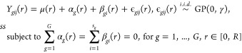
of a standard one-way ANOVA model, also known as FANOVA37 in the following way (dropping the image index j)
). Next, we consider the functional analog
of a standard one-way ANOVA model, also known as FANOVA37 in the following way (dropping the image index j)
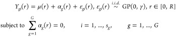 |
2 |
where μ(r), αg(r), and ϵgi(r), denote the common, group-specific, and subject-specific mean functions, respectively. GP(0, γ) denotes a Gaussian process with zero mean function and covariance function γ(r1, r2) for r1, r2 ∈ [0, R],42 where [0, R] denotes the range of r. Additional assumptions are provided in the Supporting Information.
The null hypothesis (H0) of an equal level of spatial co-occurrence at any value of the radius r across G groups can be formulated as
The total sum of squares (SST) at a particular r ∈ [0, R] can be partitioned into two components as
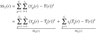 |
where SSE(r) and SSG(r) stand for within-groups and between-groups variability, respectively. To test H0, we consider the global pointwise F-type test statistic (GPF)38 given by the formula
The null distribution of Funiv can be approximated by a  distribution, where
  and
and  are suitably estimated from the data and
their forms and derivations are provided in the Supporting Information.
are suitably estimated from the data and
their forms and derivations are provided in the Supporting Information.
Note that this setup can be
readily used when we have multiple
images per subject (ngi ≥ 1) by considering a simple (or, weighted) mean of the functions
of different images corresponding to each subject, i.e., replacing Ygi(r) by  above. The crucial assumption that we would
be making with such a simplification is that the images from a particular
subject are different realizations of the same homogeneous multitype
PPP. This assumption might not be implausible, especially when the
images represent adjacent regions of the same tissue or TME. In the
results section, we refer to this approach as “SpaceANOVA Univ.”
above. The crucial assumption that we would
be making with such a simplification is that the images from a particular
subject are different realizations of the same homogeneous multitype
PPP. This assumption might not be implausible, especially when the
images represent adjacent regions of the same tissue or TME. In the
results section, we refer to this approach as “SpaceANOVA Univ.”
Multivariate Approach
In addition to the mean-based approach, when subjects have more than one image, a more sophisticated way would be to extend the one-way FANOVA model from eq 2 in the following way
 |
3 |
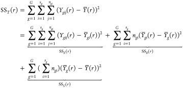
where μ(r), αg(r), βgi(r), and ϵgij(r) denote the common, group-specific, subject-specific, and image-specific mean functions, respectively. The total sum of squares can be partitioned as
 |
4 |
where  ,
,  ,
,  , and
, and  . A test statistic analogous to Funiv can be formulated as
The null distribution of Fmult can be approximated by a  distribution, where
  and
and  are suitably estimated from the data and
their forms and additional information are provided in the Supporting Information. In the results section,
we refer to this approach as “SpaceANOVA Mult.”
are suitably estimated from the data and
their forms and additional information are provided in the Supporting Information. In the results section,
we refer to this approach as “SpaceANOVA Mult.”
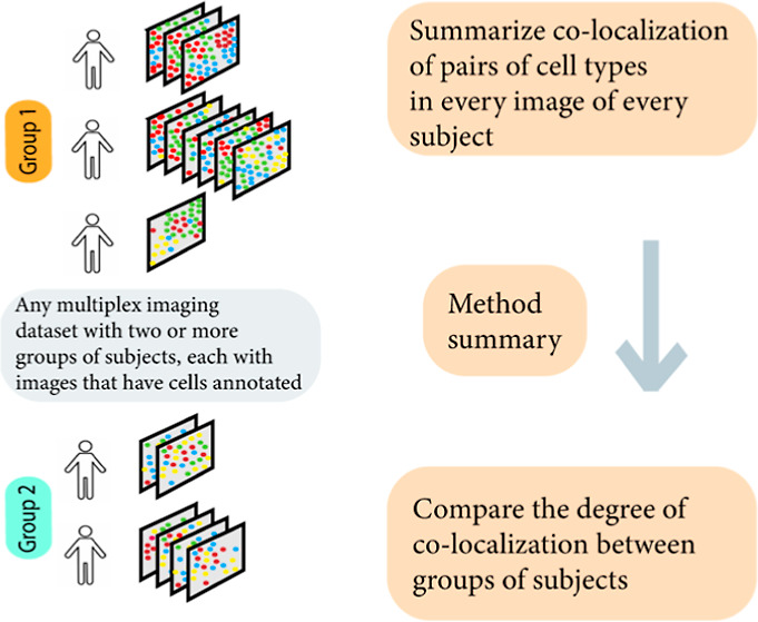
The integrals in both Funiv and Fmult are approximated using a numerical integration where r is varied across a fixed grid of values between 0 and a preselected large number R. Refer to Figure 1 for a summary of the proposed methods and refer to the Supporting Information for a discussion on how to select a suitable grid of values for r.
Figure 1.

Workflow of the proposed method. Assumptions of spatial point process are used to summarize the level of spatial co-occurrence of pairs of cell types in each image of the subjects from different groups in the form of g function and compared either using a univariate or multivariate functional ANOVA approach. Although only two groups are depicted in the figure, the method can handle any number of groups, i.e., G ≥ 2.
Adjustment to Account for Missing Tissue Regions
During the data-collection procedure, some areas of the tissue could get torn or wash away. Thus, the resulting images can have holes or blank regions in them where no cells are observed. For such images, the assumption of homogeneous multitype PPP can be too restrictive since the holes introduce an additional degree of sparseness or “in-homogeneity.” It can further lead to spatial patterns of cell types that are mere artifacts (see the Simulation section).
As alluded to, one potential solution could be to relax the assumption
of homogeneity to consider an inhomogeneous multitype PPP instead.
It would assume that the intensity of a cell type m is not constant and varies as a function of location z of an image W, i.e., λm(z) ≠ λm for z ∈ W. However,
from a theoretical point of view, such a distributional assumption
only accounts for the inhomogeneity or nonuniformity present in the
true cell-generating process and does not acknowledge an independent
source of inhomogeneity that could be artificially induced due to
data-collection challenges. In addition to that, the estimation of
λm(z) is an extremely
difficult task, one that can further bias the estimation of the K and g functions.23 There is also a risk of misinterpreting the effect of inhomogeneity
as colocalization and vice versa. Thus, we allow the assumption of
homogeneity and consider a permutation envelope-based adjustment instead.
To elaborate, we randomly switch the cell-type labels in each image
a fixed number of times (say, P = 50) and compute  every time. Then, we adjust the original g function
  as,
as,  , where
  .
.  can be interpreted as the “true”
expected value of
can be interpreted as the “true”
expected value of  under the null hypothesis of CSRI instead
of the theoretical value of 1. Thus, the adjusted g function would represent the spatial correlation that is not caused
spuriously by the nonuniform or inhomogeneous structure of the image
but is due to the process’s deviation from CSRI. A variation
of such an adjustment has been used in Wilson et al.26 Originally, Baddeley et al.39 introduced the idea of a permutation-based envelope for testing
departure from CSR in a simpler context. It is worth mentioning that
in the R package, we provide the option of
fitting inhomogeneous PPP as well but the above permutation-based
adjustment is still recommended in the presence of artificial tissue
missingness.
under the null hypothesis of CSRI instead
of the theoretical value of 1. Thus, the adjusted g function would represent the spatial correlation that is not caused
spuriously by the nonuniform or inhomogeneous structure of the image
but is due to the process’s deviation from CSRI. A variation
of such an adjustment has been used in Wilson et al.26 Originally, Baddeley et al.39 introduced the idea of a permutation-based envelope for testing
departure from CSR in a simpler context. It is worth mentioning that
in the R package, we provide the option of
fitting inhomogeneous PPP as well but the above permutation-based
adjustment is still recommended in the presence of artificial tissue
missingness.
Results
Real Data Analysis
We applied permutation-adjusted versions of SpaceANOVA Univ. and SpaceANOVA Mult. to the following real data sets,
-
1
A multiplex immunofluorescence (mIF) data set on colorectal adenoma obtained using the Vectra Polaris platform (Akoya Biosciences) at the MUSC.
-
2
An IMC data set on type 1 diabetes mellitus (T1DM).18
-
3
An mIF data set on CRC collected using the CODEX platform (Akoya Biosciences).20
To maintain the manuscript’s brevity, the analysis of the CRC data set is provided in the Supporting Information. The radius r was varied between [0, 100] with a step of size 1, i.e., r = 0, 1, 2, ..., 100 in the first two analyses. We considered 100 permutations (P = 100) in all three analyses.
Application to Colorectal Adenoma Data Set
In the colorectal adenoma study, a pathologist selected a sample of 19 lesions, recorded as conventional colorectal adenomas (tubular, villous containing), and sessile serrated lesions,43 excised from 19 patients undergoing colonoscopy between 2012 and 2014 at the Hollings Cancer Center, MUSC. We refer to these two groups of subjects or lesions as sessile serrated adenoma (SSA) or tubular/villous adenoma (TA/VA) groups. Whole slide imaging of H&E stained 5 μm thin tissue sections was performed at 20× magnification using the Vectra Polaris platform (Akoya Bioscience). Each subject has varying numbers of images (between 15 and 380) corresponding to different parts of the lesions. The overarching goal of this study is to learn commonalities and differences in immune contexture by histologic type, i.e., how SSAs differ from conventional adenomas. SSAs are known to display high cytotoxic immunogenicity (high intraepithelial lymphocytic density44) with increasing checkpoint expression as lesions progress.45 There are six immune markers: CD4, CD8, CK, FoxP3, RORgt, and Tbet, based on which different cell types, such as Th (CD4+), Tc (CD8+), Treg (CD4+FoxP3+), and Th17 (CD4+RORgt+), are identified. We applied adjusted SpaceANOVA Univ. and SpaceANOVA Mult. to understand how the pairwise spatial co-occurrence of these four immune cell types: Th, Tc, Treg, and Th17 differ between the two groups of lesions. Further data collection procedures are provided at the end of the article.
From Table 1, we
notice that the cell-type pairs: (Tc, Tc) and (Tc, Th) were detected
by both the methods to exhibit differential spatial co-occurrence
between the two groups. There were several cell type pairs, such as
(Treg, Th) and (Th, Th), that were detected only by SpaceANOVA Mult.
and their adjusted p-values were marginally higher
than 0.05 for SpaceANOVA Univ. In Figure 2, for pairs: (Treg, Th) and (Tc, Th), the
mean g function (across images) of every subject i from group g:  (from eq 4), and the overall group means:
  (from eq 4) are displayed. For (Treg, Th), the g functions in both the groups seemingly peaked at around the radius r = 10, meaning that surrounding any Treg cell, the highest
probability of finding a Th cell is at a distance of 10. The group
mean function of TA/VA appeared to be slightly higher than that of
SSA for all r ∈ [0, 100], implying that the
Treg cells were spatially closer to Th cells in TA/VA subjects as
opposed to SSA subjects. For (Tc, Th), the g functions
were mostly negative, especially for smaller values of r, implying that these two cell types avoided each other or showed
decreased spatial co-occurrence. Furthermore, comparing the group
mean function of SSA to that of TA/VA showed that the former exhibited
more negative values. It suggested that Tc and Th cells in SSA subjects
exhibited a stronger degree of avoidance or decreased spatial co-occurrence.
In Figure 2C,D, the
spatial organization of cells in two representative images from two
subjects of the two groups is shown. The figures loosely supported
these conclusions. Specifically, the images from the TA/VA subject
showed increased co-occurrence of Treg and Th cells, while in the
images from the SSA subject, Tc and Th cells appeared to have colocalized
even less compared to the other subject.
(from eq 4) are displayed. For (Treg, Th), the g functions in both the groups seemingly peaked at around the radius r = 10, meaning that surrounding any Treg cell, the highest
probability of finding a Th cell is at a distance of 10. The group
mean function of TA/VA appeared to be slightly higher than that of
SSA for all r ∈ [0, 100], implying that the
Treg cells were spatially closer to Th cells in TA/VA subjects as
opposed to SSA subjects. For (Tc, Th), the g functions
were mostly negative, especially for smaller values of r, implying that these two cell types avoided each other or showed
decreased spatial co-occurrence. Furthermore, comparing the group
mean function of SSA to that of TA/VA showed that the former exhibited
more negative values. It suggested that Tc and Th cells in SSA subjects
exhibited a stronger degree of avoidance or decreased spatial co-occurrence.
In Figure 2C,D, the
spatial organization of cells in two representative images from two
subjects of the two groups is shown. The figures loosely supported
these conclusions. Specifically, the images from the TA/VA subject
showed increased co-occurrence of Treg and Th cells, while in the
images from the SSA subject, Tc and Th cells appeared to have colocalized
even less compared to the other subject.
Table 1. Pairs of Cell Types with Adjusted p-Values < 0.05 (in Increasing Order) as Detected by Two Proposed Approaches in the Analysis of the Colorectal Adenoma Dataset.
| SpaceANOVA Univ. | cell type 1 | cell type 2 | p-value |
|---|---|---|---|
| Tc | Tc | 2.39 × 10⁻⁷ | |
| Tc | Th | 2.14 × 10⁻² | |
| Th | Tc | 3.24 × 10⁻² | |
| SpaceANOVA Mult. | Th | Th | 5.77 × 10–56 |
| Treg | Treg | 4.48 × 10–51 | |
| Th | Treg | 2.51 × 10–45 | |
| Treg | Th | 3.50 × 10–44 | |
| Th | Tc | 1.16 × 10⁻²⁸ | |
| Tc | Th | 2.09 × 10⁻²⁷ | |
| Treg | Tc | 1.75 × 10⁻²⁴ | |
| Tc | Treg | 7.24 × 10⁻²⁴ | |
| Tc | Tc | 9.41 × 10⁻²² |
Figure 2.

(A) Individual subject-level g function (averaged over images) of every subject in two groups (in the color black) and the group mean function (in the color red), for the pair of cell types: (Treg, Th). (B) Similar plot for the pair: (Tc, Th). (C,D) Cellular organization of representative images from two subjects from the groups SSA and TA/VA, respectively, where different colors correspond to different cell types.
The spatial relationship of T-cells in preinvasive colorectal lesions of different histologic types has not been previously investigated. The Treg-Th co-occurrence pattern we observed among conventional adenomas suggests a persistent immune suppressive environment. Th cells direct the adaptive immune response within the TME, determining an antitumor cytotoxic or anti-inflammatory regulatory response, potentially providing a growth advantage to the developing lesion.46 Additional information on the CD4+Foxp3+ lineage may clarify the nature of Tregs in promoting or inhibiting tumor growth in conventional lesions.47 For example, a CD4+Th17+Foxp3+ population is highly immune suppressive48 and tumor-promoting, whereas other CD4+Foxp3+ populations are associated with better prognosis.49 The inverse association between Tc and Th populations in SSA likely reflects differences in types and functions of lymphoid clustering.46 For example, the Crohn’s-like lymphoid reaction occurs peritumorally, is often densely populated with Th cells, and as it matures, assists with lymphocyte recruitment to the tumor bed. Clusters of tumor-infiltrating lymphocytes (TILs), on the other hand, emerge within the tumor nest and typically comprise Tc populations designed to kill neoplastic cells Galon et al.48 Interestingly, these lymphoid clustering patterns are also observed within microsatellite stable (MSS) and microsatellite instable (MSI+) CRC,49,50 the putative parent lesions to SSA, suggesting a shared immunologic clustering lineage. In future studies, it will be important to colocalize immune clustering to pathologically annotated regions (e.g., aggregates and dysplasia) to better inform the spatial immune clusters.
Application to the Type 1 Diabetes Data Set
In the type 1 diabetes mellitus (T1DM) data set,18 IMC technology was used to analyze pancreas tissue from four control organ donors as well as four at onset and four with long-term T1DM. We focused on the nondiabetic control group and the onset group. Each subject has varying numbers of images (between 64 and 81) and cells of 16 different types of which we studied the pairwise spatial co-occurrence of alpha, beta, delta, Th, Tc, neutrophil, and macrophage cells.
From Table 2, we notice that both methods detected two particular pairs: (beta, beta) and (delta, delta) to exhibit differential spatial co-occurrence. Investigating the estimated g functions in both groups of subjects (Figure 3), since the functions were mostly positive for the entire range of r, we concluded that in both the groups, beta and delta cells colocalized with themselves, i.e., formed clusters, more strongly in the onset group. SpaceANOVA Mult. detected several additional pairs, such as (alpha, alpha), (delta, alpha), and (Tc, beta). From Figure 4, for (alpha, delta), we noted that the g functions of both groups were mostly positive, indicating an increased or positive spatial co-occurrence. Additionally, the g functions of the onset group attained slightly higher values than the nondiabetic group implying that the cell types showed higher spatial co-occurrence in the former. The finding agreed with similar works in this field such as Gao et al.’s51 study of delta cells that revealed delta cells’ significant interaction with other endocrine cell types, alpha and beta in the context of T1DM. For (Tc, beta), we noted that the g functions of both groups were negative for smaller values of the radius r and became close to 0 and slightly higher as r increased. It indicated avoidance or decreased spatial co-occurrence of Tc and beta cells, particularly in the nondiabetic group. This result was in accordance with Damond et al.’s18 significant discovery using the same data set that Tc cells interact less with the beta cells in normal subjects but start to infiltrate the beta cell-rich areas more as T1DM progresses.
Table 2. Pairs of Cell Types with Adjusted p-Values < 0.05 (in Increasing Order) as Detected by Two Proposed Approaches in the Analysis of the Type 1 Diabetes Dataset.
| SpaceANOVA Univ. | cell type 1 | cell type 2 | p-value |
|---|---|---|---|
| delta | delta | 2.95 × 10⁻⁶ | |
| Th | Tc | 1.22 × 10⁻⁵ | |
| Th | Th | 1.83 × 10⁻⁵ | |
| Tc | Th | 9.12 × 10⁻⁵ | |
| beta | beta | 4.06 × 10⁻³ | |
| SpaceANOVA Mult | alpha | alpha | 9.09 × 10⁻³¹ |
| delta | alpha | 5.37 × 10⁻²⁹ | |
| alpha | delta | 5.48 × 10⁻²⁹ | |
| beta | beta | 4.55 × 10⁻²⁴ | |
| Tc | beta | 4.71 × 10⁻²⁴ | |
| beta | Tc | 4.23 × 10⁻²³ | |
| Tc | alpha | 5.03 × 10⁻²² | |
| alpha | Tc | 1.18 × 10⁻²⁰ | |
| beta | alpha | 7.16 × 10⁻¹⁵ | |
| alpha | beta | 7.20 × 10⁻¹⁵ | |
| Tc | Tc | 2.91 × 10⁻⁸ | |
| Tc | delta | 3.21 × 10⁻⁷ | |
| delta | delta | 6.26 × 10⁻⁷ | |
| delta | Tc | 9.32 × 10⁻⁷ | |
| delta | beta | 2.00 × 10⁻² | |
| beta | delta | 2.03 × 10⁻² |
Figure 3.

For cell type pairs (beta, beta) and (delta, delta), the image-level and subject-level (averaged over images) g functions of every subject in two groups (in the color black), and the group mean functions (in the color red) are displayed. The top panel corresponds to the subject-level and the bottom panel corresponds to the image-level functions.
Figure 4.

(A) Individual subject-level g function (averaged over images) of every subject in two groups (in the color black) and the group mean function (in the color red), for the pair of cell types: (alpha, delta). (B) Similar plot for the pair: (Tc, beta). (C,D) Cellular organization of representative images from two subjects from the groups nondiabetic and onset, respectively, where different colors correspond to different cell types.
Simulation
We evaluated the performance of both the univariate and multivariate versions of our proposed method: SpaceANOVA Univ. and SpaceANOVA Mult. in different simulation setups. For comparison, we included the two tests provided in the popular R-package SpicyR:27 one based on a linear model and the other based on a linear mixed model, called SpicyR-LM and SpicyR-Mixed, respectively. Note that the g functions were not adjusted for missing tissue regions in the first two simulations, while in the third simulation setup, we added the adjusted versions: SpaceANOVA University (adjusted) and SpaceANOVA Mult. (adjusted) in the comparison. In all three simulations, the radius r was varied between [0, 200] with a step of size 1, i.e., r = 0, 1, 2, ..., 200.
Simulation Based on the Mixed Poisson Process
We considered a variation of the framework described in Canete et al.,27 which can be loosely interpreted as a mixed PPP.23 In multiplex imaging data sets, usually, a large tissue or organ is divided into smaller nonoverlapping parts for easier and more feasible profiling, which results in multiple images per subject. To replicate that, we assumed that each subject had three images of equal area, coming from a “super”-image of size 1000 × 1000 sq. units. There were two cell types A and B with each type having JiA and JiB numbers of cells in a subject i, where JiA, JiB were randomly drawn integers from [200, 400]. To generate the superimage, the cells of type A were simulated first following a homogeneous PPP with an intensity equal to the ratio of JiA and the image area (=10002). Next, the density (or, the space-varying intensity) of cell type A was calculated using a disc kernel, where the size of the disc for each subject was either Sigma or (Sigma + Sigma-difference) depending on which group that subject belonged to. The cells of type B were then generated using an inhomogeneous PPP with the estimated density of cell type A. Note that a higher value of sigma implied lower co-occurrence or colocalization. Refer to Figures S2 and S3 of the Supporting Information to view the cellular patterns and the shape of summary functions (L and g functions) produced by the simulation mechanism (Figure 5).
Figure 5.

(A,B) Power comparison of the methods in simulation setups based on the mixed Poisson process and Neyman–Scott cluster process described in Sections Simulation Based On Mixed Poisson Process and Simulation Based On Neyman–Scott Cluster Process, respectively. The horizontal red-dotted line in every subfigure corresponds to the level α = 0.05.
From Figure 5A, we noticed that when the spatial co-occurrence was more prominent, i.e., Sigma was smaller (≤40), all the methods achieved similar performance. However, as Sigma increased, the higher power of both SpcaeANOVA Univ. and SpcaeANOVA Mult. became apparent compared to SpicyR-LM and SpicyR-Mixed. It could be partially explained by the fact that SpicyR compared the integrated value of the cumulative summary function L between the two groups. In this particular simulation, the L-functions corresponding to the two groups became very close to each other as Sigma increased, while the g functions kept exhibiting clear differences (refer to the Supporting Information Figures S2 and S3). Thus, our methods continually achieved superior power. As the number of patients increased from 50 to 100, expectedly, all of the methods achieved higher power.
Simulation Based on the Neyman–Scott Cluster Process
Next, we pursued a similar setup as in the previous section altering only the last few steps. This time, the cells were generated using a multitype Neyman–Scott cluster process23 controlled by two parameters: radius and radius-difference. A lower value of radius implied higher spatial co-occurrence. Refer to the Supporting Information for additional details.
From Figure 5B, when the radius was smaller (≤10), i.e., the degree of spatial co-occurrence was higher, SpaceANOVA Univ. and SpaceANOVA Mult. significantly outperformed SpicyR-LM and SpicyR-Mixed. As the radius increased, the latter two methods nearly caught up. Note that this observation was similar to the previous simulation setup, where for a lower degree of spatial co-occurrence, our methods were better at capturing the differences between groups. One additional point to be highlighted is that, in most of the cases, SpicyR-LM produced inflated type-1 errors. SpaceANOVA Mult. displayed slight inflation in the type-1 error in a few cases, while SpaceANOVA Univ. and SpicyR-Mixed were nearly perfect in this regard.
Simulation in the Presence of Missing Tissue Regions
In this simulation, we followed exactly the same setup described in Section Simulation Based On A Mixed Poisson Process with an additional condition that the images of subjects from group 1 would have five randomly created circular holes in them. This time, we added the adjusted versions of our tests: SpaceANOVA Univ. (adjusted) and SpaceANOVA Mult. (adjusted) to the comparison, following the steps outlined in Section Adjustment to Account for Missing Tissue Regions, with P = 50.
From Figure 6, notice that all of the previous four methods produced extremely inflated type 1 errors (close to 1), while the adjusted methods produced controlled type 1 error and were adequately powerful in all of the cases. It demonstrated the robustness of the proposed permutation envelope-based adjustment and highlighted the necessity of taking into account tissue in-homogeneity under the presence of holes or missing regions in the tissue or TME.
Figure 6.

Power comparison of the methods in the simulation setup described in Section Simulation in the Presence Of Missing Tissue Regions, involving missing tissue regions or holes. The horizontal red-dotted line in every subfigure corresponds to the level α = 0.05.
Discussion
In multiplex imaging data sets, studying the spatial co-occurrence or colocalization of different cell types is a crucial task to reveal the complex spatial biology of tissue or TME. When there are multiple groups of subjects based on a clinical or pathological phenotype, e.g., case/control or different subtypes of tissues, it becomes further possible to explore if the level of spatial co-occurrence or colocalization of different pairs of cell types varies across the groups, which could be particularly important to comprehend further facilitating our understanding of the disease pathology.
In this context, we propose a powerful method named SpaceANOVA based on the concepts of the homogeneous multitype PPP and FANOVA. SpaceANOVA has two variations, namely, SpaceANOVA Univ. and SpaceANOVA Mult., which compute spatial summary functions for every pair of cell types in images of every subject individually and then compare the functions across groups using univariate and multivariate versions of FANOVA, respectively. These tests are more general than existing approaches, which rely on oversimplifying the spatial summary functions and thereby lose power, as demonstrated in our simulations. In addition, SpaceANOVA addresses the issue of some images having missing regions, caused by data-collection challenges, using a permutation envelope-based adjustment. In a practical simulation setup, we demonstrate that not accounting for such a source of heterogeneity might introduce unwanted bias.
We have applied the proposed method to three real data sets, (1) a multiplex immunofluorescence (mIF) data set on colorectal adenoma, (2) an IMC data set on type 1 diabetes mellitus (T1DM), and (3) an mIF data set on CRC. The first mIF data set has been collected at the Medical University of South Carolina (MUSC) and is currently ongoing thorough statistical dissection that could lead to seminal discoveries. In this data set, subjects either have a sessile serrated adenoma (SSA) or a tubular/villous adenoma (TA/VA) polyp. Studying the spatial and functional properties of colorectal neoplasia is a relatively new area of research.52 From an analytic point of view, this data set is both intriguing and challenging because (a) every subject has varying numbers of images (between 15 and 380), and (b) the images are heavily plagued with the problem of missing tissue regions. We compared the spatial co-occurrence of immune cell types: Th, Tc, Treg, and Th17 between two groups of polyps, SSA and TA/VA. We found several interesting pairs of cell types to exhibit varying levels of spatial co-occurrence between these two groups. For example, Treg cells were found to be surrounded by Th cells in both groups, more prominently in the TA/VA polyps. On the other hand, Th and Tc cells exhibited avoidance or decreased spatial co-occurrence in both groups, more so in the SSA polyps. We further explored the pathological relevance of these novel findings and established concordance with the existing literature. In summary, the real data analyses demonstrate our method’s capability of discovering unique spatial associations between cell types in complex multiplex imaging data sets.
One limitation of the proposed multivariate approach is that it assumes the g functions corresponding to different images of the same subject to be independent, as they only share a common mean and no additional variance components to account for higher-order dependencies. To address this issue, instead of the two-way FANOVA model, we have tried a functional additive mixed model53 with the group label as a covariate and random effect terms capturing subject-specific dependencies, using the function “pffr” from the popular R package Refund.54 However, the model did not perform as expected because the package is admittedly not well optimized for handling a factor variable. Also, we have not explicitly discussed adjusting for covariates such as age, sex, race, and other pathologic characteristics in our proposed models. One simplistic approach would be to add the covariates directly to the mean, following the form of a simple function-on-scalar regression model.55 We would like to investigate both of these problems with further attention in future works.
Acknowledgments
The authors thank Dr. David N. Lewin for helping with the collection of the colorectal adenoma dataset.
Data Availability Statement
Software in the form of an R package named SpaceANOVA, together with simulation and real data analysis codes, is available on GitHub at this link, https://github.com/sealx017/SpaceANOVA. The publicly available data sets on type 1 diabetes and CRC, are provided as .rda files in the GitHub repository or can be accessed using their original manuscript links.
Supporting Information Available
The Supporting Information is available free of charge at https://pubs.acs.org/doi/10.1021/acs.jproteome.3c00462.
Real data analysis: additional real data results with accompanying plots and tables, simulation details: details of the simulation strategy and accompanying plots, discussion about the method: additional discussions regarding the proposed method and recommendations, results of the CRC data analysis, cellular patterns generated in the simulation setups, estimated summary functions in the simulation setups, list of p-values from the analysis of the colorectal adenoma data set, list of p-values from the analysis of the type 1 diabetes data set with two groups, list of p-values from the analysis of the type 1 diabetes data set with three groups, and list of p-values from the analysis of the CRC data set (PDF)
S.S., B.N., and E.H. were supported in part by the Biostatistics Shared Resource, Hollings Cancer Center, Medical University of South Carolina (P30 CA138313). S.S. and K.W. were supported by NCI R01 CA226086. B.N. was supported by NIMHD R21 MD016947. E.C.O. was supported in part by the Translational Science Shared Resource, Hollings Cancer Center, Medical University of South Carolina (P30 CA138313). A.A. was supported by Quantitative Methods Shared Resource (QMSR) of the South Carolina Cancer Disparities Center (SC CADRE) NCI U54 CA210962 and NLM R01 LM012517. The content is solely the responsibility of the authors and does not necessarily represent the official views of the National Institutes of Health.
The authors declare no competing financial interest.
Supplementary Material
References
- Heinzmann K.; Carter L. M.; Lewis J. S.; Aboagye E. O. Multiplexed imaging for diagnosis and therapy. Nat. Biomed. Eng. 2017, 1, 697–713. 10.1038/s41551-017-0131-8. [DOI] [PubMed] [Google Scholar]
- Burlingame E. A.; Eng J.; Thibault G.; Chin K.; Gray J. W.; Chang Y. H. Toward reproducible, scalable, and robust data analysis across multiplex tissue imaging platforms. Cells Rep. Methods 2021, 1, 100053. 10.1016/j.crmeth.2021.100053. [DOI] [PMC free article] [PubMed] [Google Scholar]
- Lewis S. M.; Asselin-Labat M. L.; Nguyen Q.; Berthelet J.; Tan X.; Wimmer V. C.; Merino D.; Rogers K. L.; Naik S. H. Spatial omics and multiplexed imaging to explore cancer biology. Nat. Methods 2021, 18, 997–1012. 10.1038/s41592-021-01203-6. [DOI] [PubMed] [Google Scholar]
- Liu C. C.; McCaffrey E. F.; Greenwald N. F.; Soon E.; Risom T.; Vijayaragavan K.; Oliveria J. P.; Mrdjen D.; Bosse M.; Tebaykin D.; et al. Multiplexed ion beam imaging: insights into pathobiology. Annu. Rev. Pathol.: Mech. Dis. 2022, 17, 403–423. 10.1146/annurev-pathmechdis-030321-091459. [DOI] [PubMed] [Google Scholar]
- Seal S.; Ghosh D. MIAMI: mutual information-based analysis of multiplex imaging data. Bioinformatics 2022, 38, 3818–3826. 10.1093/bioinformatics/btac414. [DOI] [PMC free article] [PubMed] [Google Scholar]
- Wrobel J.; Harris C.; Vandekar S.. Statistical Genomics; Springer, 2023; pp 141–168. [DOI] [PubMed] [Google Scholar]
- Giesen C.; Wang H. A. O.; Schapiro D.; Zivanovic N.; Jacobs A.; Hattendorf B.; Schüffler P. J.; Grolimund D.; Buhmann J. M.; Brandt S.; et al. Highly multiplexed imaging of tumor tissues with subcellular resolution by mass cytometry. Nat. Methods 2014, 11, 417–422. 10.1038/nmeth.2869. [DOI] [PubMed] [Google Scholar]
- Lin J.-R.; Fallahi-Sichani M.; Sorger P. K. Highly multiplexed imaging of single cells using a high-throughput cyclic immunofluorescence method. Nat. Commun. 2015, 6, 8390. 10.1038/ncomms9390. [DOI] [PMC free article] [PubMed] [Google Scholar]
- Goltsev Y.; Samusik N.; Kennedy-Darling J.; Bhate S.; Hale M.; Vazquez G.; Black S.; Nolan G. P. Deep profiling of mouse splenic architecture with CODEX multiplexed imaging. Cell 2018, 174, 968–981.e15. 10.1016/j.cell.2018.07.010. [DOI] [PMC free article] [PubMed] [Google Scholar]
- Tsujikawa T.; Kumar S.; Borkar R. N.; Azimi V.; Thibault G.; Chang Y. H.; Balter A.; Kawashima R.; Choe G.; Sauer D.; et al. Quantitative multiplex immunohistochemistry reveals myeloid-inflamed tumor-immune complexity associated with poor prognosis. Cell Rep. 2017, 19, 203–217. 10.1016/j.celrep.2017.03.037. [DOI] [PMC free article] [PubMed] [Google Scholar]
- Angelo M.; Bendall S. C.; Finck R.; Hale M. B.; Hitzman C.; Borowsky A. D.; Levenson R. M.; Lowe J. B.; Liu S. D.; Zhao S.; et al. Multiplexed ion beam imaging of human breast tumors. Nat. Med. 2014, 20, 436–442. 10.1038/nm.3488. [DOI] [PMC free article] [PubMed] [Google Scholar]
- Binnewies M.; Roberts E. W.; Kersten K.; Chan V.; Fearon D. F.; Merad M.; Coussens L. M.; Gabrilovich D. I.; Ostrand-Rosenberg S.; Hedrick C. C.; et al. Understanding the tumor immune microenvironment (TIME) for effective therapy. Nat. Med. 2018, 24, 541–550. 10.1038/s41591-018-0014-x. [DOI] [PMC free article] [PubMed] [Google Scholar]
- Schapiro D.; Jackson H. W.; Raghuraman S.; Fischer J. R.; Zanotelli V. R. T.; Schulz D.; Giesen C.; Catena R.; Varga Z.; Bodenmiller B. histoCAT: analysis of cell phenotypes and interactions in multiplex image cytometry data. Nat. Methods 2017, 14, 873–876. 10.1038/nmeth.4391. [DOI] [PMC free article] [PubMed] [Google Scholar]
- Seal S.; Wrobel J.; Johnson A. M.; Nemenoff R. A.; Schenk E. L.; Bitler B. G.; Jordan K. R.; Ghosh D. On Clustering for Cell Phenotyping in Multiplex Immunohistochemistry (mIHC) and Multiplexed Ion Beam Imaging (MIBI) Data. BMC Res. Notes 2022, 15, 215. 10.1186/s13104-022-06097-x. [DOI] [PMC free article] [PubMed] [Google Scholar]
- Shipkova M.; Wieland E. Surface markers of lymphocyte activation and markers of cell proliferation. Clin. Chim. Acta 2012, 413, 1338–1349. 10.1016/j.cca.2011.11.006. [DOI] [PubMed] [Google Scholar]
- Färkkilä A.; Gulhan D. C.; Casado J.; Jacobson C. A.; Nguyen H.; Kochupurakkal B.; Maliga Z.; Yapp C.; Chen Y.-A.; Schapiro D.; et al. Immunogenomic profiling determines responses to combined PARP and PD-1 inhibition in ovarian cancer. Nat. Commun. 2020, 11, 1459. 10.1038/s41467-020-15315-8. [DOI] [PMC free article] [PubMed] [Google Scholar]
- Keren L.; Bosse M.; Marquez D.; Angoshtari R.; Jain S.; Varma S.; Yang S. R.; Kurian A.; Van Valen D.; West R.; et al. A structured tumor-immune microenvironment in triple negative breast cancer revealed by multiplexed ion beam imaging. Cell 2018, 174, 1373–1387.e19. 10.1016/j.cell.2018.08.039. [DOI] [PMC free article] [PubMed] [Google Scholar]
- Damond N.; Engler S.; Zanotelli V. R.; Schapiro D.; Wasserfall C. H.; Kusmartseva I.; Nick H. S.; Thorel F.; Herrera P. L.; Atkinson M. A.; et al. A map of human type 1 diabetes progression by imaging mass cytometry. Cell Metabol. 2019, 29, 755–768.e5. 10.1016/j.cmet.2018.11.014. [DOI] [PMC free article] [PubMed] [Google Scholar]
- Tsakiroglou A. M.; Fergie M.; Oguejiofor K.; Linton K.; Thomson D.; Stern P. L.; Astley S.; Byers R.; West C. M. L. Spatial proximity between T and PD-L1 expressing cells as a prognostic biomarker for oropharyngeal squamous cell carcinoma. Br. J. Cancer 2020, 122, 539–544. 10.1038/s41416-019-0634-z. [DOI] [PMC free article] [PubMed] [Google Scholar]
- Schürch C. M.; Bhate S. S.; Barlow G. L.; Phillips D. J.; Noti L.; Zlobec I.; Chu P.; Black S.; Demeter J.; McIlwain D. R.; et al. Coordinated cellular neighborhoods orchestrate antitumoral immunity at the colorectal cancer invasive front. Cell 2020, 182, 1341–1359.e19. 10.1016/j.cell.2020.07.005. [DOI] [PMC free article] [PubMed] [Google Scholar]
- Welch W. J. Construction of permutation tests. J. Am. Stat. Assoc. 1990, 85, 693–698. 10.1080/01621459.1990.10474929. [DOI] [Google Scholar]
- Diggle P. J.Statistical Analysis of Spatial and Spatio-Temporal Point Patterns; CRC Press: Boca Raton, FL, 2013. [Google Scholar]
- Baddeley A.; Rubak E.; Turner R.. Spatial Point Patterns: Methodology and Applications with R; CRC Press: Boca Raton, FL, 2015. [Google Scholar]
- Bull J. A.; Macklin P. S.; Quaiser T.; Braun F.; Waters S. L.; Pugh C. W.; Byrne H. M. Combining multiple spatial statistics enhances the description of immune cell localisation within tumours. Sci. Rep. 2020, 10, 18624. 10.1038/s41598-020-75180-9. [DOI] [PMC free article] [PubMed] [Google Scholar]
- Vipond O.; Bull J. A.; Macklin P. S.; Tillmann U.; Pugh C. W.; Byrne H. M.; Harrington H. A. Multiparameter persistent homology landscapes identify immune cell spatial patterns in tumors. Proc. Natl. Acad. Sci. U.S.A. 2021, 118, e2102166118 10.1073/pnas.2102166118. [DOI] [PMC free article] [PubMed] [Google Scholar]
- Wilson C.; Soupir A. C.; Thapa R.; Creed J.; Nguyen J.; Segura C. M.; Gerke T.; Schildkraut J. M.; Peres L. C.; Fridley B. L. Tumor immune cell clustering and its association with survival in African American women with ovarian cancer. PLoS Comput. Biol. 2022, 18, e1009900 10.1371/journal.pcbi.1009900. [DOI] [PMC free article] [PubMed] [Google Scholar]
- Canete N. P.; Iyengar S. S.; Ormerod J. T.; Baharlou H.; Harman A. N.; Patrick E. spicyR: Spatial analysis of in situ cytometry data in R. Bioinformatics 2022, 38, 3099–3105. 10.1093/bioinformatics/btac268. [DOI] [PMC free article] [PubMed] [Google Scholar]
- Vu T.; Wrobel J.; Bitler B. G.; Schenk E. L.; Jordan K. R.; Ghosh D. SPF: a spatial and functional data analytic approach to cell imaging data. PLoS Comput. Biol. 2022, 18, e1009486 10.1371/journal.pcbi.1009486. [DOI] [PMC free article] [PubMed] [Google Scholar]
- Ripley B. D. The second-order analysis of stationary point processes. J. Appl. Probab. 1976, 13, 255–266. 10.2307/3212829. [DOI] [Google Scholar]
- Legendre P.; Fortin M. J. Spatial pattern and ecological analysis. Vegetatio 1989, 80, 107–138. 10.1007/BF00048036. [DOI] [Google Scholar]
- Gatrell A. C.; Bailey T. C.; Diggle P. J.; Rowlingson B. S. Spatial point pattern analysis and its application in geographical epidemiology. Trans. Inst. Br. Geogr. 1996, 21, 256–274. 10.2307/622936. [DOI] [Google Scholar]
- Kerscher M.Statistical Physics and Spatial Statistics: The Art of Analyzing and Modeling Spatial Structures and Pattern Formation; Springer, 2000, pp 36–71. [Google Scholar]
- Anselin L.; Cohen J.; Cook D.; Gorr W.; Tita G. Spatial analyses of crime. Crim. Justice 2000, 4, 213–262. [Google Scholar]
- Osher N.; Kang J.; Krishnan S.; Rao A.; Baladandayuthapani V. SPARTIN: a Bayesian method for the quantification and characterization of cell type interactions in spatial pathology data. Front. Genet. 2023, 14, 1175603. 10.3389/fgene.2023.1175603. [DOI] [PMC free article] [PubMed] [Google Scholar]
- Dayao M. T.; Trevino A.; Kim H.; Ruffalo M.; D’Angio H. B.; Preska R.; Duvvuri U.; Mayer A. T.; Bar-Joseph Z. Deriving spatial features from in situ proteomics imaging to enhance cancer survival analysis. Bioinformatics 2023, 39, i140–i148. 10.1093/bioinformatics/btad245. [DOI] [PMC free article] [PubMed] [Google Scholar]
- Cui E.; Crainiceanu C. M.; Leroux A. Additive functional Cox model. J. Comput. Graph. Stat. 2021, 30, 780–793. 10.1080/10618600.2020.1853550. [DOI] [PMC free article] [PubMed] [Google Scholar]
- Zhang J.-T.Analysis of Variance for Functional Data; CRC Press: Boca Raton, FL, 2013. [Google Scholar]
- Smaga Ł.; Zhang J.-T. Linear hypothesis testing with functional data. Technometrics 2019, 61, 99–110. 10.1080/00401706.2018.1456976. [DOI] [Google Scholar]
- Baddeley A.; Diggle P. J.; Hardegen A.; Lawrence T.; Milne R. K.; Nair G. On tests of spatial pattern based on simulation envelopes. Ecol. Monogr. 2014, 84, 477–489. 10.1890/13-2042.1. [DOI] [Google Scholar]
- Wallace K.; El Nahas G. J.; Bookhout C.; Thaxton J. E.; Lewin D. N.; Nikolaishvili-Feinberg N.; Cohen S. M.; Brazeal J. G.; Hill E. G.; Wu J. D.; et al. Immune Responses Vary in Preinvasive Colorectal Lesions by Tumor Location and Histology. Cancer Prev. Res. 2021, 14, 885–892. 10.1158/1940-6207.CAPR-20-0592. [DOI] [PMC free article] [PubMed] [Google Scholar]
- Illian J.; Benson E.; Crawford J.; Staines H.. Principal component analysis for spatial point processes—assessing the appropriateness of the approach in an ecological context. Case Studies In Spatial Point Process Modeling; Springer Science & Business Media, 2006; Vol. 185, pp 135–150. [Google Scholar]
- Banerjee S.; Gelfand A. E.; Finley A. O.; Sang H. Gaussian predictive process models for large spatial data sets. J. R. Stat. Soc., B: Stat. Methodol. 2008, 70, 825–848. 10.1111/j.1467-9868.2008.00663.x. [DOI] [PMC free article] [PubMed] [Google Scholar]
- Nagtegaal I. D.; Odze R. D.; Klimstra D.; Paradis V.; Rugge M.; Schirmacher P.; Washington K. M.; Carneiro F.; Cree I. A. The 2019 WHO classification of tumours of the digestive system. Histopathology 2020, 76, 182–188. 10.1111/his.13975. [DOI] [PMC free article] [PubMed] [Google Scholar]
- Rau T. T.; Atreya R.; Aust D.; Baretton G.; Eck M.; Erlenbach-Wünsch K.; Hartmann A.; Lugli A.; Stöhr R.; Vieth M.; et al. Inflammatory response in serrated precursor lesions of the colon classified according to WHO entities, clinical parameters and phenotype–genotype correlation. J. Pathol.: Clin. Res. 2016, 2, 113–124. 10.1002/cjp2.41. [DOI] [PMC free article] [PubMed] [Google Scholar]
- Acosta-Gonzalez G.; Ouseph M.; Lombardo K.; Lu S.; Glickman J.; Resnick M. B. Immune environment in serrated lesions of the colon: intraepithelial lymphocyte density, PD-1, and PD-L1 expression correlate with serrated neoplasia pathway progression. Hum. Pathol. 2019, 83, 115–123. 10.1016/j.humpath.2018.08.020. [DOI] [PMC free article] [PubMed] [Google Scholar]
- Rozek L. S.; Schmit S. L.; Greenson J. K.; Tomsho L. P.; Rennert H. S.; Rennert G.; Gruber S. B. Tumor-infiltrating lymphocytes, Crohn’s-like lymphoid reaction, and survival from colorectal cancer. J. Natl. Cancer Inst. 2016, 108, djw027. 10.1093/jnci/djw027. [DOI] [PMC free article] [PubMed] [Google Scholar]
- Maoz A.; Dennis M.; Greenson J. K. The Crohn’s-like lymphoid reaction to colorectal cancer-tertiary lymphoid structures with immunologic and potentially therapeutic relevance in colorectal cancer. Front. Immunol. 2019, 10, 1884. 10.3389/fimmu.2019.01884. [DOI] [PMC free article] [PubMed] [Google Scholar]
- Galon J.; Costes A.; Sanchez-Cabo F.; Kirilovsky A.; Mlecnik B.; Lagorce-Pagès C.; Tosolini M.; Camus M.; Berger A.; Wind P.; et al. Type, density, and location of immune cells within human colorectal tumors predict clinical outcome. Science 2006, 313, 1960–1964. 10.1126/science.1129139. [DOI] [PubMed] [Google Scholar]
- De Smedt L.; Lemahieu J.; Palmans S.; Govaere O.; Tousseyn T.; Van Cutsem E.; Prenen H.; Tejpar S.; Spaepen M.; Matthijs G.; et al. Microsatellite instable vs stable colon carcinomas: analysis of tumour heterogeneity, inflammation and angiogenesis. Br. J. Cancer 2015, 113, 500–509. 10.1038/bjc.2015.213. [DOI] [PMC free article] [PubMed] [Google Scholar]
- Chang K.; Willis J.; Reumers J.; Taggart M.; San Lucas F.; Thirumurthi S.; Kanth P.; Delker D.; Hagedorn C.; Lynch P.; et al. Colorectal premalignancy is associated with consensus molecular subtypes 1 and 2. Ann. Oncol. 2018, 29, 2061–2067. 10.1093/annonc/mdy337. [DOI] [PMC free article] [PubMed] [Google Scholar]
- Gao R.; Yang T.; Zhang Q. δ-cells: The neighborhood watch in the islet community. Biology 2021, 10, 74. 10.3390/biology10020074. [DOI] [PMC free article] [PubMed] [Google Scholar]
- Lin J.-R.; Wang S.; Coy S.; Chen Y. A.; Yapp C.; Tyler M.; Nariya M. K.; Heiser C. N.; Lau K. S.; Santagata S.; et al. Multiplexed 3D atlas of state transitions and immune interaction in colorectal cancer. Cell 2023, 186, 363–381.e19. 10.1016/j.cell.2022.12.028. [DOI] [PMC free article] [PubMed] [Google Scholar]
- Scheipl F.; Staicu A.-M.; Greven S. Functional additive mixed models. J. Comput. Graph. Stat. 2015, 24, 477–501. 10.1080/10618600.2014.901914. [DOI] [PMC free article] [PubMed] [Google Scholar]
- Goldsmith J.; Crainiceanu C. M.; Caffo B.; Reich D. Longitudinal penalized functional regression for cognitive outcomes on neuronal tract measurements. J. R. Stat. Soc., C: Appl. Stat. 2012, 61, 453–469. 10.1111/j.1467-9876.2011.01031.x. [DOI] [PMC free article] [PubMed] [Google Scholar]
- Ramsay J. O.; Silverman B. W.. Functional Data Analysis; Springer-Verlag: New York, 2005. [Google Scholar]
Associated Data
This section collects any data citations, data availability statements, or supplementary materials included in this article.
Supplementary Materials
Data Availability Statement
Software in the form of an R package named SpaceANOVA, together with simulation and real data analysis codes, is available on GitHub at this link, https://github.com/sealx017/SpaceANOVA. The publicly available data sets on type 1 diabetes and CRC, are provided as .rda files in the GitHub repository or can be accessed using their original manuscript links.