

Abstract

The present study investigates the applicability of the inlet boundary species Lewis number (combined effect of molecular and flow diffusion) for the nonpremixed moderate and intense low oxygen dilution (MILD) flames. A modified reactive solver named modifiedReactingFoam is developed by including the enthalpy flux in the energy equation and using modified model constants in OpenFOAM. The present solver is tested on the delft-jet-in-hot-coflow burner operating under a moderate and intense low oxygen dilution combustion environment. Along with the flame with Reynolds number 4100, eight other jet-in-hot-coflow flames are simulated to test the capability of the present proposed solver. The main aim of the current work is to investigate the efficacy of the proposed solver in predicting the velocity field, temperatures, and flame lift-off height for the considered flames with a significant reduction in computational time. The predictions with the modified eddy dissipation concept model are improved. However, a significant deviation is still observed in the downstream direction of the burner. The numerical simulations are performed with methane Lewis numbers of 0.9–1.14 by keeping the respective constant Lewis numbers for the inlet boundary species. The modifiedReactingFoam predictions at a methane Lewis number of 1.12 are in very close agreement with the experimental results. The maximum deviation in lift-off heights is within ±3% of the experimental results. The present modified solver outperformed the other combustion models in the literature and reduced the computational time up to 10 times with a combination of DLBFoam compared to the inbuilt solver.
1. Introduction
The stringent pollution norms and problems related to pollutant emissions from conventional combustion led to the development of new combustion technologies. Initially, the researchers introduced the concept of high reactant temperatures, focusing mainly on preheating and regeneration techniques applied to the air input system for reducing pollutant emissions. This is called “high-temperature air combustion” (HITAC).1 In HITAC, the air is preheated above the self-ignition temperature of the mixture and primarily focused on improving the thermal efficiency of the combustors. On the other hand, flameless combustion works similarly to the HITAC, with a different mode of operation in which there is no appearance of visible flame within the combustor. Wiinning and Wiinning2 have achieved flameless combustion with the low-temperature gradient in an industrial furnace using gaseous fuel and referred to it as flameless oxidation (FLOX). The colorless distributed combustion (CDC) method to enhance mixing and the dispersed reaction zone was utilized by Arghode and Gupta3 to obtain very low NOx and CO emissions. However, CDC is based on high combustion intensities and lower residence time than HITAC. Cavaliere and De Joannon4 are the ones who first coined the term MILD combustion using the partially stirred reactor (PSR) model, in which the reactants are supplied above the self-ignition temperature, and the temperature increment inside the combustor is lower than the self-ignition temperature of the fuel. Some of the significant factors influencing achieving the MILD combustion are fuel type, dilution level, preheating temperature of the reactants, and operating conditions (pressure).5,6 The geometrical shape of the combustor also plays a crucial role in achieving MILD combustion by enhancing the internal recirculation of combustion products.7,8
Various numerical techniques are extensively used to study the reaction physics of MILD combustion. Reynolds-averaged Navier–Stokes (RANS) models have been extensively used in numerical simulations of MILD combustion in jet-in-hot-coflow (JHC) burners. Christo and Dally9,10 have applied various models such as the Flamelet model, eddy dissipation concept (EDC) model, and transported probability density function (PDF) model, by adopting RANS simulations to validate the experimental results of methane-hydrogen MILD combustion stabilized in the JHC burner.11 They pointed out that the EDC model outperformed the Flamelet model. Sarras et al.12 conducted a detailed analysis of the performance of EDC with DRM19 chemical mechanism and PDF/3D-flamelet generated manifold (FGM) models in predicting experimental data of the delft JHC (DJHC) burner.13 They have concluded that the EDC coupled with the DRM 19 model restricted its efficiency due to its inability to account for the temperature changes at the coflow inlet. These fluctuations can be refined using the conveyed PDF approaches for simulating complex finite-rate chemistry. The benefit of using this technique is that the mean reaction rate is accurately addressed. However, a considerable amount of computing time is associated with integrating response rates in the EDC model.14 The EDC model is the refined version of the eddy dissipation model (EDM) which allows detailed chemical processes to be included in turbulent flows. EDC and EDM models are compared in the previous studies presented in the literature.9,15,16 The infinitely fast-rate chemistry assumption is invalid in the MILD combustion since the chemical reaction occurs in a broader zone, and the chemical reaction rate is slower.17 Therefore, the results of a numerical investigation of MILD combustion by fast-rate chemistry are unsatisfactory. Kulkarni and Polifke18 considered the considerable computational time of the EDC model. They modeled the DJHC burner using large eddy simulation (LES) and a PDF method with stochastic fields and two mixture fractions. The temperature distributions are over predicted, but the estimated lift-off height agrees with the experimental results for the different fuel jet Reynolds numbers. Ihme and See19 extended the Flamelet/progress variable technique to the Adelaide burner using a second mixture fraction in LES. The predictions significantly improved by adding a second mixture fraction than a formulation using a single mixture fraction. They observed that the single mixing fraction could not appropriately represent the fluctuation in the coflow. The limitations of a single PDF are considered, and Darbyshire and Swaminathan20 simulated the joint PDF of the mixture fraction and a progress variable with a specified covariance. The correlations that Darbyshire and Swaminathan20 suggested for the joint PDF make the calculated mean temperature of a stratified v-flame slightly better than it would be with the traditional statistically independent PDF formulation. The Favre-averaged chemical source term in a turbulent reacting flow is calculated by conditional source term estimation (CSE) using conditional flow parameter averages.21 The transport equations are solved in conditional momentum closure (CMC) to determine the conditional averages.22 Labahn et al.21 studied the DJHC flame using the CSE model.
In comparison to EDC23 and LES-stochastic fields,18 CSE performed better in terms of temperature predictions in the radial direction.21 Nevertheless, toward the exit of the burner, radial distributions of the temperature with the CSE model significantly deviated from the experimental results. Kim et al.24 applied CMC to the Adelaide burner by employing a single mixture fraction and a modified PDF model and achieved accurate predictions. However, it is found that the NO concentration is underestimated. Overall, various advanced combustion modeling techniques have recently been developed to study MILD combustion characteristics. Overall, it is observed that most of the combustion models have certain issues in predicting the temperature and emissions of the MILD combustion flames. Since turbulent transport often dominates molecular diffusion in turbulent flow, it is the usual practice to compute the molecular diffusion terms using more straightforward methods while ensuring no significant errors in the computations. The molecular diffusion is essential in the lower turbulent region and should not be ignored. The heat release causes the fluid to expand, which can lead to a reduction in vorticity and the destruction of local vortex tubes.25 However, this presents an opportunity to study the effects of heat on fluid dynamics and to potentially discover new phenomena. In other words, combustion helps to reduce turbulence and promote laminar flow. Although molecular transport is becoming more critical than turbulent transport, it is still possible to use simplified assumptions in combustion simulations, such as assuming equal and constant diffusivities for all species.
Characterizing the transport processes emerging within the gaseous mixtures, especially in premixed combustion, heavily depends on the Lewis number (Le).26−29 It is frequently described as the ratio of the Schmidt number and the Prandtl number.30 In this study, Le is equivalently regarded as the thermal-to-mass diffusivity ratio of the individual species. The development of asymptotic theories31−33 supported early experimental findings on flame propagation, stability, and extinction characteristics. These theories showed that flame stretch, unequal heat, and species diffusion (Le) significantly affect the overall combustion phenomenon. Recently, interest in flexible fuel burners has grown, prompting more research on flame stability, blow-off occurrences, and flame characteristics. With the imbalance between heat and mass diffusion, such burners must operate with fuels with varying Lewis numbers, substantially influencing the stabilization mechanism and flame propagation. The given fuel diffusion and heat loss effects are coupled with the flow nonuniformities, resulting in a variation in flame behavior. A higher flame temperature (more than adiabatic flame temperature) is observed in the case of premixed flame with Le ≤ 1, while in the case of Le > 1, a lower flame temperature is observed.34 Along with nonunity Le effects, a preferential diffusion effect is generated by the variations in species diffusivities, generating a regional imbalance in the basic mass fractions, thereby altering the local stoichiometry. Such effects have recently been investigated in turbulent premixed methane–air35 and methane–hydrogen–air36 flames stabilized on a bluff body. Premixed counterflow flames with varied Lewis numbers have previously been investigated for propane, methane, and hydrogen–air mixtures.37 Furthermore, Lewis number-based analysis is conducted in the literature on premixed flames to observe the flame characteristics.37,38 The Lewis number-based analysis is carried out in these investigations by varying the fuel and oxidizer combination proportions and blending the other fuels. In these cases, the premixed flame effective Lewis number is calculated by using a linear approximation (Leeffective = Xi·Lei, where Xi is the volume fraction of ith species and Lei is individual Le of ith species in the mixture). This indicates that the Lewis number is a characteristic of a generic fuel–air mixture when diffusing in a particular environment. In the case of nonpremixed MILD combustion, the reactants travel together before the reaction takes place, similar to the premixed case. Therefore, Le has a crucial role in the reaction physics of either nonpremixed or premixed cases of MILD combustion. In the literature, various techniques like considering a nonunity Le, Hirschfelder–Curtiss diffusion model, Soret effects, and applying a dynamic turbulence model with a variable turbulent Prandtl number are studied39 for the case of a nonpremixed flame. These studies focused on pool fire flame analysis with global reaction using numerical simulations. However, the analysis did not include the detailed chemical mechanism and performed a few numerical simulations without providing the details of the considered Le. Furthermore, several additional studies on the use of the Le number in the OpenFOAM environment have been conducted for conventional flames40,41 and internal combustion applications.42 Moreover, combustion physics of open pool fires or conventional flames much differs from those of MILD combustion flames. Smith et al.43 identified exciting insights into the effects of molecular diffusion in nonpremixed turbulent jet flames of H2/CO2 in the air. The study demonstrated the significant impact of differential diffusion on the flame. The MILD combustion regime’s specific conditions of reduced heat release and oxygen concentration offer intriguing possibilities for exploring combustion beyond traditional methods. Damping of turbulence eddies and relaminarization are both carried out at various levels. The molecular transport strongly affects the MILD combustion regime, and it is important to consider differential diffusion in CFD modeling of the H2/CH4 flame, as reported by Christo and Dally.10 The studies demonstrate how including differential diffusion in flame modeling can impact radial distributions for temperature, CO2, and CO mass fraction. As stated, this topic has received scant attention in the literature for MILD conditions. In other words, no exhaustive research has been conducted on the effect of MILD combustion under nonpremixed conditions. Many research works are conducted on premixed and very limited on nonpremixed flames. The present study reports a Le-based computational analysis for the first time for the nonpremixed flames. Hence, in this study, an artificial treatment (by considering Lewis number variation of individual species in the literature) of Le is carried out to see the variation in flame characteristics. In the present study, all the flames are operated with three fuel mixtures at various fuel jet Reynolds numbers. The three considered fuel mixtures comprise of significantly higher quantity of methane (more than 80% in volume) in the fuel jet. Henceforth, the Le of methane is varied for validation by keeping the Le of all other inlet boundary species in the fuel and coflow constant.
The present study focuses on the EDC model to improve the solver’s capabilities in OpenFOAM 8. It is found that the EDC model with detailed chemical kinetic mechanisms for MILD combustion provides more accurate predictions. Despite this, because of the over-projected mean reaction rates, the temperature is often overpredicted using the original EDC model constants.10,23,44,45 Therefore, the main goal of this study is to change the turbulence and combustion model constants in the OpenFOAM built-in reactive solver by using detailed chemical mechanism. The EDC combustion model predictions with modified model constants are improved.9,17 However, a considerable deviation in the combustion variables is observed based on the earlier research in the literature,33,34 and the assumption of a unity Lewis number in the EDC model is focused on in this study to improve the solver’s capabilities further.
Numerical simulations for MILD combustion with essential solvers with detailed mechanisms involved more complications and required more computational time. The significant disadvantages of the basic EDC model are the requirement of substantial computational time with detailed chemical kinetic mechanisms and the early reaction of fuel.46 Hence, the present work helps overcome these disadvantages of the EDC model. They are addressed by incorporating the dynamic load balancing and a zonal reference mapping mechanism in parallel simulations proposed by Tekgül et al.47 It effectively reduces the computational time by ∼10 times concerning the inbuilt reactive solver using detailed chemistry in OpenFOAM.
Furthermore, an individual Lewis number analysis is performed by considering individual inlet boundary species (fuel jet and coflow) Le from the experimental data available in the literature. Since no built-in OpenFOAM solver is available to meet the needs of the proposed method under consideration, a novel solver is proposed by incorporating the two solvers’ algorithms with the built-in reacting solver available in OpenFOAM to study the DJHC burner flame behavior. In addition to the proposed solver, the effective model constants for turbulence and combustion models are modified based on the literature for the MILD combustion case. They are reported separately as a modified EDC model to see the shift of the solution from its original constants. The effects of the individual Lewis number on the DJHC-I 4100 flame characteristics are studied by considering a Le range from 0.9 to 1.14 for methane while keeping other inlet boundary species’ Le constant. The numerical comparisons of the combustion parameters revealed that a case of Le = 1.12 for methane yields accurate results when compared with Oldenhof et al.’s experimental results.13,48 The finalized Le of 1.12 for the methane fuel with the modified EDC model is applied to different flames of the DJHC-I 8800 with DNG and the DJHC-I 3000, 4500, and 5000 with fuel-I and fuel-II.13,48 The capability of the current modified reacting solver is tested for these cases.
2. Mathematical Modeling
In the present
work, the Favre-averaged turbulence modeling is
incorporated with a typical two-equation k–ε
model, and a standard wall function is imposed along the wall boundaries.
The governing equations decide the flow pattern, and the significance
of each component is governed by the model constants used in turbulence
modeling. One of the significant parameters in the turbulence equation
is turbulent viscosity  , where ε represents the turbulent
dissipation; k represents the turbulent kinetic energy;
and cμ is a constant. The constants
in the turbulence modeling cμ, σk, and cμ, σε decide the strength of the diffusion
of turbulent kinetic energy and dissipation rate, respectively. The
constants cμ and c1 decide the production rate, while cμ and c2 decide the
destruction rate for both the turbulent kinetic energy and the dissipation
rate, respectively.
, where ε represents the turbulent
dissipation; k represents the turbulent kinetic energy;
and cμ is a constant. The constants
in the turbulence modeling cμ, σk, and cμ, σε decide the strength of the diffusion
of turbulent kinetic energy and dissipation rate, respectively. The
constants cμ and c1 decide the production rate, while cμ and c2 decide the
destruction rate for both the turbulent kinetic energy and the dissipation
rate, respectively.
The characteristics of the flame are determined by mixing (length scale) and reaction rate in any combustion problem. The EDC model considers that the fluid state is determined by the fraction of the fine structure states and the surrounding state.49 The fraction of the flow occupied by such regions can be represented by eqs 1–350 as follows:
| 1 |
| 2 |
| 3 |
where c*γ represents the volume fraction constant; c*τ denotes the time-scale constant; and ν represents the kinematic viscosity. The above expression can be written in terms of the Kolmogorov length scale (η) and the Taylor length scale (λ) as
| 4 |
The mean resident time scale characterizes the mass transmission time scale between the fine structures and their surroundings, and it is expected to be as follows:
| 5 |
The constants CD1 and CD2 are the primary determinants of the time and length scale in the computational domain under consideration with values of 0.135 and 0.5, respectively. For the standard EDC model, the secondary constants c*γ and c*τ are considered to be 2.1377 and 0.4083, respectively. Christo and Dally10 propose an EDC model suitable for MILD combustion. As a result, it is selected for the modeling of the interaction between turbulence and reactions in this study. In the MILD combustion simulations, the constant for turbulence production rate (Cε1) in the k–ε with standard wall function model is changed from 1.44 to 1.6.9 In the EDC model, primary determinants of time scale and volume fraction are changed from 0.135 to 0.6638 and 0.5 to 9.3987, respectively. The secondary constants of time scale and volume fraction are changed from 0.4083 to 1.77 and 2.1377 to 2.0, respectively, as suggested by Kuang et al.17 In the present study, the change in turbulence and combustion model constants are considered as a modified EDC model with unity Lewis number consideration.
The following species mass conservation equation is used to examine molecular diffusion in multicomponent mechanisms:25
| 6 |
where ρ represents the mixture density; v⃗ represents the velocity vector of the mixture; p represents the pressure; Yi represents the mass fraction of ith species; Vi denotes the diffusion velocity of ith species; and wi represents the mass reaction rate of ith species. Calculating the diffusion velocities is necessary to solve eq 6. In general, diffusion velocities may be estimated by using one of two methods. The first Fick’s law is used as the initial approximation. The second, more precise method involves resolving the multicomponent diffusion equations and deriving Vi from the results. Following specific changes to eq 6, ignoring thermal diffusion, body forces, and pressure-induced diffusion, and using the first and generalized Fick’s law, the mass conservation equation for turbulent flow and in Reynolds-average form can be written as follows for the steady state:51
| 7 |
| 8 |
where J⃗ represents the diffusive mass flux vector of the ith species; Dim represents the mass diffusion coefficient for the ith species; Sci represents the turbulent Schmidt number. The RHS of the eq 8 first term represents the molecular diffusivity term, and the second one is the turbulent diffusive term. Using the Lewis number of unity as a definition, the equal diffusion coefficient is determined as follows:
| 9 |
where λ represents the thermal conductivity of local mixture; CP represents the local specific heat; Lei represents the Lewis number of ith species. A similar kind of study has been performed by Mardani et al.51 and Azarinia and Mahdavy-Moghaddam52 on the JHC burner under the constant thermal diffusivity and unity Lewis number consideration in the species conservation equation. These studies stated that the consideration of the diffusivities of the species in the domain for numerical calculation will improve the computational results and the cost. It is also stated that the inclusion of the diffusion effect on the flames operating under lower oxygen conditions significantly affects the numerical solution. The Lewis number of species i and the Prandtl number of the species i may be used to express the Schmidt number as Sci = LeiPri. This implies that how the Lewis number is considered in the conservation equations is connected to the various methods for describing the diffusion coefficient. In the present study, the thermal diffusivities of the species are also considered in eq 7, and it becomes
| 10 |
The enthalpy flux (Fh) component, a function of the Lewis number, is also added to the species transport equation in the EDC model to incorporate the Lewis number. The modified enthalpy equation is as follows:
| 11 |
| 12 |
| 13 |
| 14 |
where h represents the specific total enthalpy of the mixture; τ represents the stress tensor; μ represents the dynamic viscosity; I represents the identity tensor; λ represents the mixture thermal conductivity; T represents the temperature; hi represents the specific total enthalpy of ith species; and N represents the number of species. The considered Lewis number is an effective Lewis number appearing in the expression for the combined effect of laminar and turbulent diffusion. In these equations, the diffusivity is always the result of the sum of the laminar and turbulent contributions. In the case of high Reynolds number flow, the laminar contribution is significantly less and may be omitted. This is typically not the case for the JHC burner studies, and both should be preserved. Hence, the combined effect is considered by taking the effective Lewis number. The current work thoroughly investigates the influence of the turbulence and combustion constants as well as the Lewis number on the prediction of various parameters under the MILD condition.
Since there is no built-in solver in OpenFOAM to feed the individual Lewis number, the required new variables are created in the library and the above equations are modified in reactive solver in the OpenFOAM 8. In addition to the above governing equations, the direct integration approach is used to find the chemical source term in the reactive flow.53 The discrete ordinate (DO) radiation model54 is used in the present study with a weighted sum of the gray gas model (WSGGM) to compute the radiative heat transfer through appropriate prediction of the emission and absorption coefficients.
Tekgül et al.47 introduced a new solver called DLBFoam in the OpenFOAM environment to reduce the computational time by an order of magnitude as compared to the default EDC model. DLBFoam is an OpenFOAM open-source library. It incorporates dynamic load balancing and a zonal reference mapping mechanism in the parallel simulations that result in fast chemistry computations. It also includes an analytical Jacobian formulation and enhanced ordinary differential equation (ODE) solution methods with an increased computational efficiency. DLBFoam uses a Python library and reference mapping technique to accelerate the chemical reactions in the numerical simulations. The implementation of the DLBFoam algorithms in the numerical simulation requires thermos input files in the OpenFOAM format as well as analytical Jacobian C subroutines generated by the pyJac. Figure 1 shows a schematic of the different steps involved in the modified reactive solver. The iterative solutions for mass, momentum, species, and energy conservation laws are determined. The changes made in the inbuilt reactingFoam solver are highlighted by a yellow line in the flowchart.
Figure 1.
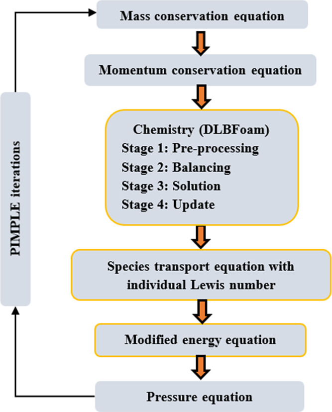
Various steps of the modifiedReactingFoam solver.
3. Computational Methodology
The following section provides thorough information about the computational domain and operating parameters under consideration. It also details the grid independence test and model validation of the combustion parameters under different flow conditions, as described in detail. Three criteria are specified to identify the convergence of the solution. First, ensure that the residuals of all variables are less than 10–6. The second step is to verify that the residuals of all variables have stabilized and are no longer changing as the model is iterated. The third step is to ensure that with iterations the maximal temperature fluctuation at the peak temperature location is less than 3 K at three distances of 30, 60, and 120 mm from the nozzle.
3.1. Computational Domain and Boundary Conditions
In the present study, the experimental conditions (DJHC flame and Delft burner) of Oldenhof et al.13,48 are considered for the validation of the solver with the Lewis numbers of the individual species in the fuel jet. The Delft burner consists of a hot coflow chamber of 82.8 mm diameter. The fuel jet of 4.5 mm diameter is centrally located in the hot coflow. The present numerical results are compared with the experimental results of Oldenhof et al.,13,48 operated with Dutch natural gas (DNG). The fuel and oxidizer composition with respective Lewis numbers of the individual species of the DNG and coflow are listed in Table 1. In the experiments of Oldenhof et al.,13,48 composition of the coflow is fed from the secondary premixed burner operated with natural gas.
Table 1. Boundary Conditions13 and Effective Lewis Numbers Considered for the Inlet Boundary Species.
| species | fuel (DNG) volume % | fuel-I volume % | fuel-II volume % | coflow volume % | effective Le |
|---|---|---|---|---|---|
| CH4 | 81.3 | 85 | 81 | 0 | 0.9–1.14 |
| C2H6 | 3.7 | 4 | 0 | 1.67 | |
| O2 | 0 | 6.659 | 1.1 | ||
| N2 | 14.4 | 15 | 15 | 74.222 | 1.04 |
| H2O | 0 | 12.656 | 0.89 | ||
| CO2 | 0 | 6.462 | 1.39 | ||
| rest | 0.6 | 0 |
The temperature and velocity profiles of the coflow are observed as nonuniform due to the nature of the burner design. Therefore, the radial temperature and velocity distributions for the coflow inlet are obtained,13 and polynomial equations for temperature (eq 15) and velocity (eq 16) are generated using MATLAB curve fitting. The generated profiles are used for numerical simulations. The inlet velocity of the fuel jet is 34 m/s, and the corresponding Reynolds number is 4100. The initial conditions in the computational domain are set to atmospheric conditions. The domain is a 100 mm radius cylindrical wedge and 250 mm along the axis.12 The computational domain is extended in the radial direction up to 100 mm by considering the air entrainment zone.
| 15 |
| 16 |
In general, the combustion chamber of a nonpremixed burner consists of premixed, partially premixed, and nonpremixed zones. Hence, the Lewis numbers for the fuel jet (methane) are considered to be from lean to rich conditions in the literature. Also, the molecular kinetic hypothesis states that each species’ diffusivity generally depends on all other species.51 Hence, the Lewis numbers are considered for the inlet boundary species to perform the numerical simulations,26,49,55 as shown in Table 1. A change in Le for a particular species results in a relative diffusivity change in the given medium. Giving each species in the chemical mechanism a unique Lewis number may increase the computational time and complexity. As a result, in the current work, the individual Le for the inlet boundary species investigated, particularly the primary fuel jet (methane), are examined to determine how they affect numerical predictions. Therefore, the Le for the methane fuel is altered, while the Le for other inlet boundary species is kept constant, as given in Table 1. The Le of the CH4 jet varies from 0.9 to 1.12 with a step of 0.01. The finalized Le for the DNG fuel with DJHC-I 4100 flame is again tested for the various fuels (Table 1) at different Reynolds numbers to elucidate the capabilities of the proposed methodology for nonpremixed flames. The present work uses the detailed chemical mechanism GRI Mech 3.0 for numerical simulations. The 2D-numerical simulations are performed using a modifiedReactingFoam solver by feeding individual Lewis numbers for the fuel jet and other inlet boundary species. The fuel enters the domain at 34 m/s and the coflow conditions are given as per the experimental measurements.13,23
3.2. Grid Independence Test
The 2D computational domain, as shown in Figure 2, is discretized into smaller quadratic lateral volume elements. Since the number of cells and node connectivity in the computation domain profoundly affect the solution and computational cost, meshing is decisive in getting an accurate solution from the simulations. Therefore, to get robust solutions, simulations are done with three different discretized domains, with G1, G2, and G3 having 48,192, 68,980, and 98,551 nodes, respectively, from several simulations using three different discretized domains. The grid-independent analysis considers the radial distributions of the velocity, temperature, and oxygen concentrations at an axial location of 30, 60, 90, and 120 mm. From the grid independence test, it was observed that the simulations with G2 and G3 grids show similar results with a deviation of less than 1%, as shown in Figure 3. Therefore, the G2 mesh containing 68,980 nodes is considered for further analysis in this study.
Figure 2.

Schematic of the computational domain with boundary conditions.
Figure 3.

Radial distributions of (a) velocity, (b) temperature, and (c) O2 mass fractions at various axial locations for different grid sizes.
4. Model Validation
The solution accuracy of the numerical simulations depends on the turbulent and combustion models, model constants, chemical mechanism, and other boundary conditions considered. However, in the present study, the simulation results are analyzed in two stages: change in model constants defined as modified EDC model (Mod_EDC) and effect of Lewis numbers in modified EDC model (Mod_EDC_Var Le) by keeping chemical mechanism and boundary conditions constant. The radial distributions of various combustion characteristics are analyzed at the different axial locations. The present numerical results of combustion and flow parameters are compared with the experimental studies of Oldenhof et al.13,48 The capability of the current modifiedReactingFoam solver is compared with some other combustion models in the literature, such as CSE, EDC, and PDF models.12,21
The flow characteristics of the burner are one of the driving parameters for mixing the fuel and the oxidizer. In this study, the standard k–ε model is implemented by observing the distributive turbulence in the burner. The flow characteristics, mainly velocity distribution and turbulent kinetic energy, are compared with the experimental results and other combustion models (EDC and PDF) implemented by Sarras et al.12 The comparison of the experimental and the numerical results for the radial distribution of the velocity at various axial locations is shown in Figure 4. Flow turbulence is one of the critical elements of reacting flow that determines how quickly fuel and oxidizer combine. Turbulence in the flow is closer to the fuel nozzle and minimizes it downstream. In a reacting flow, the downstream flow characteristics are dominated by molecular diffusion rather than flow turbulence. However, the proposed solver considers both turbulent and molecular diffusions to capture accurate results. The local fluctuation of the velocity field within the domain primarily determines the flow characteristics. Therefore, the radial distributions of velocity fields at different axial locations using the present modified solver are compared with the experimental findings of Oldenhof et al.13 The computed velocity distributions closely agree with the experimental results for a methane Lewis number of 1.12 with the modified EDC model. Figure 5 shows the distribution of the turbulent kinetic energy (k) in the radial direction at axial positions of 15 and 60 mm from the burner nozzle. The computed turbulent kinetic energy (k) using the present modified solver is compared with the experimental results13 and other numerical models EDC12 and PDF12 for a methane Lewis number of 1.12 (Figure 5).
Figure 4.

Comparison of experimental and present numerical results of the radial distribution of velocity at various axial locations for methane Le = 1.12.
Figure 5.

Comparison of radial distribution of turbulent kinetic energy at the axial locations of (a) 15 and (b) 60 mm for methane Le of 1.12 with experimental results48 and other combustion models.12 Adopted in part with permission from ref. (12) Copyright 2014 Springer.
The computational results for all of the models show trends similar to the experimental results. However, in the case of the EDC model, the turbulent kinetic energy is underpredicted (20%) at 15 mm and overpredicted (16%) at 60 mm axial distance. A reduction of 70% in error is observed upon modification of the model constants in the EDC model (Mod EDC). Whereas in the case of the PDF model, the predictions for peak values of the turbulent kinetic energy are relatively better than those of the EDC model near the fuel jet (at a 15 mm axial location). However, the downstream EDC of the burner EDC outperformed the PDF model, as shown in Figure 5b. The trend of the turbulent kinetic energy is slightly shifted toward the air entrainment side for the PDF model. The predictions of the present modified solver with variable Le are in close agreement with the experimental results. These predictions are comparatively better than those of the EDC, modified EDC, and PDF models over the entire domain. The present modified solver demonstrates a favorable agreement with experimental results in predicting velocity and jet spread rate within the computational domain compared to other models.
The combustion process plays a crucial role in determining the temperature and distribution of various species within a given domain. The temperature distributions serve as indicators of the energy release rates in the computational domain at the local level. Consequently, a comparison is made between the temperature distributions at different axial positions and the corresponding experimental outcomes. The present study reports on the enhancement of temperature predictions achieved through utilizing the modified EDC model and the modified EDC model incorporating Le, which are discussed independently. Figure 6 shows how the experimental results,48 EDC,12 3D-PDF,12 and CSE21 models for the temperature distribution in the radial direction at different axial locations compare with each other. The EDC model findings show a trend similar to the experimental results. However, a peak temperature is observed in all of the cases due to the nature of the fast-rate chemistry. A comparison is made between the temperature predictions of the EDC model, as reported in the literature, at distances of 60 and 120 mm from the fuel jet of the burner. In both cases, the EDC model tended to overestimate the magnitude of the observed experimental values. When the model constants are changed in the EDC model, the predicted temperatures are very close to the actual temperatures up to 60 mm from the fuel jet. These regions are identified as having higher turbulence. A deviation in temperature predictions occurred when the burner. Upon additional implementation of the Lewis number for the inlet boundary species, it is observed that the temperature predictions are highly consistent throughout the burner. Therefore, it is evident that modifications in model constants facilitate the estimation of combustion parameters in regions of higher turbulence, where the flow turbulence is higher than that of molecular diffusion.
Figure 6.

Radial distribution of temperature and comparison with various models at different axial locations (z) (a) 30, (b) 90, (c) 60, and (d) 120 mm for DJHC-I 4100 for methane Le = 1.12. Adopted in part with permission from ref. (12) Copyright 2014 Springer. Adopted in part with permission from ref. (21) Copyright 2015 Elsevier.
However, as we move downstream, molecular diffusion becomes dominant and is explicable by considering the individual Lewis numbers of the inlet boundary species. The PDF model’s temperature predictions outperformed the EDC model. The prediction of the temperature distributions near the fuel exit with the CSE model is in good agreement with the experimental results in the radial direction, as shown in Figure 6a. The CSE model predictions agree with the EDC and PDF models in the downstream direction. However, it is slightly away from the experimental measurements (Figure 6c,d)). For a methane Lewis number of 1.12, it is interesting to note that the predictions of the present modified reacting solver are more in line with the experimental results than those of other models such as CSE,21 EDC,12 and PDF.12 A small overprediction of the peak temperature is observed at the 30 mm axial location perhaps because the present modified reaction solver is derived from the EDC model. DLBFoam contributed to a significant reduction in computational time, up to 10 times, in a specific case involving a detailed mechanism. On the other hand, without the assistance of DLBFoam, Mod_EDC and Mod_EDC_Var Le cases exhibited computational times of 76 and 82 h, respectively, as shown in the Figure 7. Upon implementing DLBFoam for these cases, the computational times decreased to 8.3 h for Mod_EDC and 9.1 h for Mod_EDC_Var Le.
Figure 7.

Execution times for the current solver with and without DLBFoam.
5. Results and Discussion
The flame’s diffusion depends on molecular and flow turbulence, as mentioned in the preceding section. The flow turbulence is captured in computational simulations by choosing suitable models and their corresponding model constants. The results of computing the current solver with modified combustion and turbulence model constants (modified EDC) showed an improvement in the predictions of various parameters. The findings of the modified EDC model demonstrated that an accurate prediction of the temperature distribution downstream of the burner still needed to be achieved. The transport equation must consider the species’ molecular and turbulent diffusion to improve the predictions of the numerical simulations. Mardani et al.51 previously reported the impact of molecular diffusion of the species on combustion characteristics. According to Mardani et al.51 adding each species’ diffusivity to the transport equation significantly improved the predictions’ accuracy. However, the complexity of the numerical simulation increases with a greater computing time. In addition, it is also shown that when flow turbulence is taken into account for the species in the transport equation, the computational results in areas with more turbulence (especially when the Reynolds number is high) are much better. Considering all of these factors in this study, the diffusion of the species at the molecular and turbulent levels is combined by providing individual Lewis numbers for the species in the transport equation. In order to accelerate the computational time, individual Lewis numbers for the border species are taken into account. The optimum methane Le is identified by comparing the radial distribution of several variables at various axial locations in the computational domain. The finalized methane Le is verified with eight other flames to check the stability and accuracy of the present modified solver (Mod_EDC_Var Le/modified ReactingFoam). This section presents the effect of Le of the main fuel jet (methane) on the flame characteristics, such as lift-off height, temperature variation, heat release rate, and other parameters.
5.1. Variation of Flame Lift-Off Heights
In the experimental study of Oldenhof et al.,13 the flame lift-off height is determined by considering the probability of chemiluminescence from an ignition kernel (flame pockets). The likelihood of detecting a flame pocket at a particular axial height above the fuel jet nozzle is the probability of burning (Pb2).13 Pb2 = 0.5 is the lift-off height location considered during the experiments of Oldenhof et al.13 since this function increases monotonically with height. The ignition kernels need to be represented in detail in the numerical models. As a result, a direct quantitative comparison with the experimental observations is challenging. Therefore, this necessitates the development of a new definition of lift-off height.12 Different criteria have been proposed in the literature to calculate the flame lift-off height for the JHC flames. The parameters considered for the calculation of lift of height are the peak values of the mean temperature, which is equal to half of the maximum temperature in radial profile,8 the lowest point of temperature in iso-contour at 1350 K,56 and OH mass fraction. In the present study, the lift-off height is assumed to be located where the OH mass fraction is 0.001. A similar approach has also been adopted by De et al.23 and Kulkarni and Polifke18 while studying the hot coflow burner with basic EDC and LES models, respectively.
Figure 8 depicts the variation of the OH mass fraction for the considered range of methane Lewis numbers. The minimum mass fraction of 0.001 is regarded for its lift-off height appearance. The values indicated in the figure ranging from 0.00165 to 0.00150 represent the peak magnitudes of the OH mass fraction in the domain for Le 0.9 to 1.12, respectively. In the case of lower Le, the ignition started earlier than the unity Le case. Therefore, the flame gets stabilized at a lower position. The flame shifted downstream with an increased Lewis number. At Le = 0.9, the flame anchored at an axial distance of 72 mm, whereas at Le = 1.12, the flame stabilized at 82 mm (Figure 8). It is observed from the experiments of Oldenhof et al.13 that the actual lift-off height for DJHC-I 4100 lies approximately within 80 mm of the fuel jet exit plane. The peak value of OH is observed to decrease with an increase in the methane Lewis number.
Figure 8.

Variation of lift-off heights with various Lewis numbers for DJHC-I 4100.
Figure 9 shows the measurement of flame lift-off height by Oldenhof et al.48 (Figure 9a), the OH mass fraction contour with a minimum mass fraction of 0.001, and the respective heat release rate (HRR) with a minimum magnitude of 1.2 × 10⁸ J/m2. The present computational domain is considered 3 mm from the fuel nozzle. Therefore, the lift of height of 85 mm predicted using the current numerical model is well validated with the experimental results at Le = 1.12 for methane (Figure 9).
Figure 9.
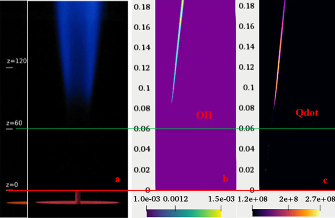
Measurement of lift-off height (a) experimental results of Oldenhof et al.,48 (b) variation of OH, and (c) variation of HRR in the computational domain for DJHC-I 4100.
Figure 9 shows the variation of the lift-off heights for different fuels at various Reynolds numbers (Re) of the fuel jet. It is observed that the lift-off height decreases with an increase in jet Re due to increased mixing of the fuel jet. The calculated lift-off heights from the numerical simulations with the proposed methodology are in good agreement with the measurements of Oldenhof et al.13,48 for all fuel compositions and the Re range. The overall deviation is within ±3% of the experimental results, as shown in Figure 10.
Figure 10.

Comparison of lift-off heights for various flames on DJHC-I.
5.2. Temperature and Heat Release Rate Variation
The effect of the individual Lewis number on the reaction zone of the present nonpremixed flame is analyzed. Figure 11 describes the temperature distribution in the computational domain for various Lewis numbers. The parametric difference between the different methane Lewis numbers can be observed in Figure 12. The increase in the methane Lewis number indicates that either the thermal diffusivity of the fuel (methane) increases or the mass diffusivity of the fuel (methane) dominates. Therefore, for the lower Lewis number case, the fuel diffusivity in the coflow stream is more significant than for the higher Lewis number case. The increased diffusivity of the fuel enhances the mixing of fuel and oxidizer, which results in the stabilization of the flame at a faster rate than in the lower diffusivity case, thus increasing the peak temperature. In the present case, peak temperatures of 1850 and 1770 K are observed at methane Le values of 0.9 and 1.12, respectively, as shown in Figure 11. The peak temperature decreased with an increase in the methane Lewis number. A similar trend is observed for the variation of OH peak (mass fraction) values with methane Lewis number. Mizomoto et al.57 have shown that the flame peak temperature rises if Le < 1 and remains nearly the same or changes marginally for Le ≥ 1, similar to the observations of the present study.
Figure 11.

Temperature contours are for various Lewis numbers.
Figure 12.

Variation of HRR in the computational domain for various methane Lewis numbers.
The variation of the heat release rate in the computational domain for various methane Lewis numbers is shown in Figure 12. The interpretation of the HRR follows a trend similar to temperature and OH variation with methane Lewis numbers. The burning characteristics of the hydrocarbon fuel are governed by the OH radical production rate, an indicator of the overall reaction zone.58 The produced OH radicals further react with the available oxygen and release heat. The numerical simulation results presented here show good agreement among OH production, HRR, and temperature within the computational domain.
Figure 13a shows the temperature variation at the exit of the computational domain for two different methane Le cases. The energy release is relatively higher for the lower methane Le case than the higher methane Le case. Therefore, higher peak temperatures are observed for the lower methane Le cases. The variation in the peak temperature for two different methane Le (Le = 0.9 and 1.12) is around 80 K, and this region lies between 30 and 45 mm in the radial direction. Higher temperature regions enhance the formation of NOx. However, the concept of MILD combustion results in lower and distributed peak temperature regions and thus enables the control of NOx formation in the combustion zone. Implementing individual Lewis numbers for nonpremixed flames helps obtain accurate results in the case of MILD combustion. The temperature variation obtained from the simulations is mainly due to the variation in the Lewis numbers.
Figure 13.

Variation of (a) temperature and (b) mass fraction of CH4 and O2 along the radial direction at the exit. (c) Temperature for various Le at z = 60 mm for DJHC-I 4100. (d) Focused window of the temperature from the radial temperature distributions in (c).
Figure 13c shows the variation of the radial temperature distribution at an axial location of 60 mm for different methane Le cases. These computational results are compared with the experimental results of Oldenhof et al.48 at the same location. The computational results for different methane Le cases are validated in the reaction zone with experimental data. However, a peak temperature (maximum of 10%) is detected with the present modifiedReactingFoam solver. A significantly higher temperature value is observed for the lower methane Le values. This temperature peak is reduced with an increase in the methane Le. For methane Le = 1.12, the peak value is almost minimized, and the predictions agree with the experimental results, as shown in the encircled zone of Figure 13d. For instance, at 12.6 mm from the central axis, peak temperatures of 1586 and 1420 K are observed for a case of methane Le = 0.9 and the experimental results, respectively. An overprediction of ∼28% is observed for this case. At the same time, 1454 and 1420 K peak temperatures are observed for the case of methane Le = 1.12 and the experimental results, respectively. The variation in the peak temperatures is nearly 4%, which is relatively small. Therefore, lower discrepancies in the computational and experimental results are observed. Nevertheless, the results with a methane Le of 1.12 are in good agreement with the experimental results in this zone.
Figure 14 shows the OH mass fraction, temperature, and equivalence ratio (φ) contours in the computational domain for the methane Le = 1.12 case. The dotted line on the three contours represents the φ = 1 (stoichiometric) contour. This domain is divided into three zones: fuel-rich, mixing/reacting, and fuel-lean zones. The left side of the dashed line is the fuel-rich zone, near the premises of the dashed line is the mixing/reacting zone, and the right side (dashed line) is the fuel-lean zone.
Figure 14.

Variation of (a) OH mass fraction, (b) temperature, and (c) equivalence ratio in the domain for DJHC-I 4100 flames. In all the contours dashed line indicates the stoichiometric (φ = 1), and the black colored line indicates the OH mass fraction at 0.001.
It is observed that combustion (reaction zone) started in the mixing/reacting zone and propagated in the radial direction. In the fuel-rich zone, the oxygen availability is significantly lower. Hence, no reaction is identified in this zone. However, the temperature rise is observed due to the mixing of fuel and the hot coflow. The fuel and coflow interact in the mixing zone and form the mixture within the flammability limits. It initiates a reaction and stabilizes a thin reaction zone within the domain. In the lean zone, the unburned mixture is further carried out downstream. The flame is anchored as an inverted conical flame. In the outer zone, coflow and the surrounding air entrainment cool the coflow. These results show what the proposed modified solver can capture both preferential and differential diffusion when the fuel Lewis number is considered for nonpremixed flames in the MILD combustion regime. The extension of the solver in the open-source code (OpenFOAM), without any additional model complexities or assumptions, is the primary advantage of the present approach over other combustion models in the literature.
6. Conclusions
The present work highlights the limitations of the basic EDC model and proposes the construction of a new solver called modifiedReactingFoam. In OpenFOAM 8, the modified solver uses DLBFoam algorithms and allows the user to feed the individual Lewis numbers of the respective species in reactingFoam. The experimental results of MILD combustion cases on the Delft burner are considered for validating the capabilities of the present solver and its accuracy. In this study, the influence of the individual Lewis number on achieving accurate predictions of the MILD combustion regime is studied in detail. Some of the noteworthy contributions of this study are presented as follows:
-
1.
The implemented modifiedReactingFoam solver included with DLBFoam used Python-based libraries for solving chemistry and reduced the computational time by 10 times compared to the conventional EDC solver.
-
2.
In the present model, the constants for the primary determinants of time scale and volume fraction and secondary determinants of time scale and volume fraction are changed since these constants are significantly affecting the numerical findings of the MILD combustion (Figure 10).
-
3.
The lift-off height of around 80 mm is observed from the experimental measurements of Oldenhof et al.13 The present model is well validated for all the cases of DJHC-I flames (Figure 10).
-
4.
The Lewis number varied from 0.9 to 1.14; it was observed that the experimental and computational results are very well validated with Le = 1.12 of the methane fuel.
-
5.
Some crucial parameters such as velocity, turbulent kinetic energy, and temperatures are in close agreement with the experimental results compared to the previous models (EDC, CSE, and PDF).
The main benefit of the present approach is that the reacting solver can be extended to nonpremixed flames by adding an individual inlet boundary species Le to the open-source code (OpenFOAM) without any additional modeling assumptions or complexity. This makes it suitable for complex MILD combustion flames.
Acknowledgments
The authors (M.S. and V.M.R.) would like to acknowledge the support from the Prime Minister Research Fellowship (PMRF) and the Indian Institute of Technology Kharagpur. V.M.R. is also thankful to Seoul National University for the BK21 FOUR project ‘2023.
The authors declare no competing financial interest.
References
- Katsuki M.; Hasegawa T. The science and technology of combustion in highly preheated air. Symp. (Int.) Combust. 1998, 27, 3135–3146. 10.1016/S0082-0784(98)80176-8. [DOI] [Google Scholar]
- Wünning J. A.; Wünning J. G. Flameless oxidation to reduce thermal no-formation. Prog. Energy Combust. Sci. 1997, 23, 81–94. 10.1016/S0360-1285(97)00006-3. [DOI] [Google Scholar]
- Arghode V. K.; Gupta A. K. Development of High Intensity CDC Combustor for Gas Turbine Engines. Appl. Energy 2011, 88 (3), 963–973. 10.1016/j.apenergy.2010.07.038. [DOI] [Google Scholar]
- Cavaliere A.; De Joannon M. Mild Combustion. Prog. Energy Combust. Sci. 2004, 30, 329–366. 10.1016/j.pecs.2004.02.003. [DOI] [Google Scholar]
- Mohapatra S.; Garnayak S.; Lee B. J.; Elbaz A. M.; Roberts W. L.; Dash S. K.; Reddy V. M. Numerical and Chemical Kinetic Analysis to Evaluate the Effect of Steam Dilution and Pressure on Combustion of N-Dodecane in a Swirling Flow Environment. Fuel 2021, 288, 119710 10.1016/j.fuel.2020.119710. [DOI] [Google Scholar]
- Srinivasarao M.; Jun D.; Jik B.; Reddy V. M. Numerical Analysis of the Enrichment of CH 4/H 2 in Ammonia Combustion in a Hot Co-Flow Environment. Int. J. Hydrogen Energy 2023, 288, 119710 10.1016/j.fuel.2020.119710. [DOI] [Google Scholar]
- Reddy V. M.; Katoch A.; Roberts W. L.; Kumar S. Experimental and Numerical Analysis for High Intensity Swirl Based Ultra-Low Emission Flameless Combustor Operating with Liquid Fuels. Proc. Combust. Inst. 2015, 35 (3), 3581–3589. 10.1016/j.proci.2014.05.070. [DOI] [Google Scholar]
- Kumar S.; Paul P. J.; Mukunda H. S. Prediction of Flame Liftoff Height of Diffusion/Partially Premixed Jet Flames and Modeling of Mild Combustion Burners. Combust. Sci. Technol. 2007, 179 (10), 2219–2253. 10.1080/00102200701407887. [DOI] [Google Scholar]
- Christo F. C.; Dally B. B.; Application of Transport PDF Approach for Modelling MILD Combustion. In 15th Australasian Fluid Mechanics Conference; 2004. [Google Scholar]
- Christo F. C.; Dally B. B. Modeling Turbulent Reacting Jets Issuing into a Hot and Diluted Coflow. Combust. Flame 2005, 142 (1–2), 117–129. 10.1016/j.combustflame.2005.03.002. [DOI] [Google Scholar]
- Dally B. B.; Karpetis A. N.; Barlow R. S. Structure of Turbulent Non-Premixed Jet Flames in a Diluted Hot Coflow. Proc. Combust. Inst. 2002, 29 (1), 1147–1154. 10.1016/S1540-7489(02)80145-6. [DOI] [Google Scholar]
- Sarras G.; Mahmoudi Y.; Arteaga Mendez L. D.; Van Veen E. H.; Tummers M. J.; Roekaerts D. J. E. M. Modeling of Turbulent Natural Gas and Biogas Flames of the Delft Jet-in-Hot-Coflow Burner: Effects of Coflow Temperature, Fuel Temperature and Fuel Composition on the Flame Lift-off Height. Flow, Turbul. Combust. 2014, 93 (4), 607–635. 10.1007/s10494-014-9555-3. [DOI] [Google Scholar]
- Oldenhof E.; Tummers M. J.; van Veen E. H.; Roekaerts D. J. E. M. Ignition Kernel Formation and Lift-off Behaviour of Jet-in-Hot-Coflow Flames. Combust. Flame 2010, 157 (6), 1167–1178. 10.1016/j.combustflame.2010.01.002. [DOI] [Google Scholar]
- Sharma D.; Mahapatra S.; Garnayak S.; Arghode V. K.; Bandopadhyay A.; Dash S. K.; Reddy V. M. Development of the Reduced Chemical Kinetic Mechanism for Combustion of H2/CO/C1-C4 Hydrocarbons. Energy Fuels 2021, 35 (1), 718–742. 10.1021/acs.energyfuels.0c02968. [DOI] [Google Scholar]
- Jin X.; Zhou Y. Numerical Analysis on Microscopic Characteristics of Pulverized Coal Moderate and Intense Low-Oxygen Dilution Combustion. Energy Fuels 2015, 29 (5), 3456–3466. 10.1021/acs.energyfuels.5b00088. [DOI] [Google Scholar]
- Vascellari M.; Cau G. Influence of Turbulence-Chemical Interaction on CFD Pulverized Coal MILD Combustion Modeling. Fuel 2012, 101, 90–101. 10.1016/j.fuel.2011.07.042. [DOI] [Google Scholar]
- Kuang Y.; He B.; Wang C.; Tong W.; He D. Numerical Analyses of MILD and Conventional Combustions with the Eddy Dissipation Concept (EDC). Energy 2021, 237, 121622 10.1016/j.energy.2021.121622. [DOI] [Google Scholar]
- Kulkarni R. M.; Polifke W. LES of Delft-Jet-In-Hot-Coflow (DJHC) with Tabulated Chemistry and Stochastic Fields Combustion Model. Fuel Process. Technol. 2013, 107, 138–146. 10.1016/j.fuproc.2012.06.015. [DOI] [Google Scholar]
- Ihme M.; See Y. C. LES Flamelet Modeling of a Three-Stream MILD Combustor: Analysis of Flame Sensitivity to Scalar Inflow Conditions. Proc. Combust. Inst. 2011, 33 (1), 1309–1317. 10.1016/j.proci.2010.05.019. [DOI] [Google Scholar]
- Darbyshire O. R.; Swaminathan N. A Presumed Joint Pdf Model for Turbulent Combustion with Varying Equivalence Ratio. Combust. Sci. Technol. 2012, 184 (12), 2036–2067. 10.1080/00102202.2012.696566. [DOI] [Google Scholar]
- Labahn J. W.; Dovizio D.; Devaud C. B. Numerical Simulation of the Delft-Jet-in-Hot-Coflow (DJHC) Flame Using Conditional Source-Term Estimation. Proc. Combust. Inst. 2015, 35 (3), 3547–3555. 10.1016/j.proci.2014.07.027. [DOI] [Google Scholar]
- Klimenko A. Y.; Bilger R. W. Conditional Moment Closure for Turbulent Combustion. Prog. Energy Combust. Sci. 1999, 25, 595. 10.1016/S0360-1285(99)00006-4. [DOI] [Google Scholar]
- De A.; Oldenhof E.; Sathiah P.; Roekaerts D. Numerical Simulation of Delft-Jet-in-Hot-Coflow (DJHC) Flames Using the Eddy Dissipation Concept Model for Turbulence-Chemistry Interaction. Flow, Turbul. Combust. 2011, 87 (4), 537–567. 10.1007/s10494-011-9337-0. [DOI] [Google Scholar]
- Kim S. H.; Huh K. Y.; Dally B. Conditional Moment Closure Modeling of Turbulent Nonpremixed Combustion in Diluted Hot Coflow. Proc. Combust. Inst. 2005, 30 (1), 751–757. 10.1016/j.proci.2004.08.161. [DOI] [Google Scholar]
- Tien J. S. Principles of Combustion. Combust. Flame 1988, 73 (3), 337. 10.1016/0010-2180(88)90028-4. [DOI] [Google Scholar]
- Bouvet N.; Halter F.; Chauveau C.; Yoon Y. On the Effective Lewis Number Formulations for Lean Hydrogen/Hydrocarbon/ Air Mixtures. Int. J. Hydrogen Energy 2013, 38 (14), 5949–5960. 10.1016/j.ijhydene.2013.02.098. [DOI] [Google Scholar]
- Wu C. K.; Law C. K. On the Determination of Laminar Flame Speeds from Stretched Flames. Symp. (Inst.) Combust. 1985, 20 (1), 1941–1949. 10.1016/S0082-0784(85)80693-7. [DOI] [Google Scholar]
- Law C. K.; Ishizuka S.; Cho P. On the Opening of Premixed Bunsen Flame Tips. Combust. Sci. Technol. 1982, 28 (3–4), 89–96. 10.1080/00102208208952545. [DOI] [Google Scholar]
- Sato J. Effects of Lewis Number on Extinction Behavior of Premixed Flames in a Stagnation Flow. Symp. (Inst.) Combust. 1982, 19 (1), 1541–1548. 10.1016/S0082-0784(82)80331-7. [DOI] [Google Scholar]
- Webb R. L. Standard Nomenclature for Mass Transfer Processes. Int. Commun. Heat Mass Transfer 1990, 17 (5), 529–535. 10.1016/0735-1933(90)90001-Z. [DOI] [Google Scholar]
- Sivashinsky G. I. On a Distorted Flame Front as a Hydrodynamic Discontinuity. Acta Astronaut. 1976, 3, 889–918. 10.1016/0094-5765(76)90001-1. [DOI] [Google Scholar]
- Matalon M. On Flame Stretch. Combust. Sci. Technol. 1983, 31 (3–4), 169–181. 10.1080/00102208308923638. [DOI] [Google Scholar]
- Clavin P. Dynamic Behavior of Premixed Flame Fronts in Laminar and Turbulent Flows. Prog. Energy Combust. Sci. 1985, 11, 1. 10.1016/0360-1285(85)90012-7. [DOI] [Google Scholar]
- Sharpe G. J Combustion Physics. By K. Law Chung. Cambridge University Press, 2006. 738 pp. ISBN 0521 870526. £55. J. Fluid Mech. 2007, 588, 474–475. 10.1017/s0022112007007860. [DOI] [Google Scholar]
- Dunn M. J.; Barlow R. S. Effects of Preferential Transport and Strain in Bluff Body Stabilized Lean and Rich Premixed CH4/Air Flames. Proc. Combust. Inst. 2013, 34 (1), 1411–1419. 10.1016/j.proci.2012.06.070. [DOI] [Google Scholar]
- Barlow R. S.; Dunn M. J.; Magnotti G. Preferential Transport Effects in Premixed Bluff-Body Stabilized CH4/H2 Flames. Combust. Flame 2015, 162 (3), 727–735. 10.1016/j.combustflame.2014.09.006. [DOI] [Google Scholar]
- Salusbury S. D.; Bergthorson J. M. Maximum Stretched Flame Speeds of Laminar Premixed Counter-Flow Flames at Variable Lewis Number. Combust. Flame 2015, 162 (9), 3324–3332. 10.1016/j.combustflame.2015.05.023. [DOI] [Google Scholar]
- Vance F. H.; Shoshin Y.; van Oijen J. A.; de Goey L. P. H. Effect of Lewis Number on Premixed Laminar Lean-Limit Flames Stabilized on a Bluff Body. Proc. Combust. Inst. 2019, 37 (2), 1663–1672. 10.1016/j.proci.2018.07.072. [DOI] [Google Scholar]
- Maragkos G.; Beji T.; Merci B. Advances in Modelling in CFD Simulations of Turbulent Gaseous Pool Fires. Combust. Flame 2017, 181, 22–38. 10.1016/j.combustflame.2017.03.012. [DOI] [Google Scholar]
- Zhou D.; Zhang H.; Yang S. A Robust Reacting Flow Solver with Computational Diagnostics Based on OpenFOAM and Cantera. Aerospace 2022, 9 (2), 102. 10.3390/aerospace9020102. [DOI] [Google Scholar]
- Yang Q.; Zhao P.; Ge H. ReactingFoam-SCI: An Open Source CFD Platform for Reacting Flow Simulation. Comput. Fluids 2019, 190, 114–127. 10.1016/j.compfluid.2019.06.008. [DOI] [Google Scholar]
- Muhammad N.; Zaman F. D.; Mustafa M. T. OpenFOAM for Computational Combustion Dynamics. Eur. Phys. J. Spec. Top. 2022, 231 (13–14), 2821–2835. 10.1140/epjs/s11734-022-00606-6. [DOI] [Google Scholar]
- Smith L. L.; Dibble R. W.; Talbot L.; Barlow R. S.; Carter C. D. Laser Raman Scattering Measurements of Differential Molecular Diffusion in Turbulent Nonpremixed Jet Flames of H2 CO2 Fuel. Combust. Flame 1995, 100 (1–2), 153–160. 10.1016/0010-2180(94)00066-2. [DOI] [Google Scholar]
- Shabanian S. R.; Medwell P. R.; Rahimi M.; Frassoldati A.; Cuoci A. Kinetic and Fluid Dynamic Modeling of Ethylene Jet Flames in Diluted and Heated Oxidant Stream Combustion Conditions. Appl. Therm. Eng. 2013, 52 (2), 538–554. 10.1016/j.applthermaleng.2012.12.024. [DOI] [Google Scholar]
- Evans M. J.; Medwell P. R.; Tian Z. F. Modeling Lifted Jet Flames in a Heated Coflow Using an Optimized Eddy Dissipation Concept Model. Combust. Sci. Technol. 2015, 187 (7), 1093–1109. 10.1080/00102202.2014.1002836. [DOI] [Google Scholar]
- Ishizuka S.; Law C. K. An Experimental Study on Extinction and Stability of Stretched Premixed Flames. Symp. (Int.) Combust. 1982, 19 (1), 327–335. 10.1016/S0082-0784(82)80204-X. [DOI] [Google Scholar]
- Tekgül B.; Peltonen P.; Kahila H.; Kaario O.; Vuorinen V. DLBFoam: An Open-Source Dynamic Load Balancing Model for Fast Reacting Flow Simulations in OpenFOAM. Comput. Phys. Commun. 2021, 267, 108073 10.1016/j.cpc.2021.108073. [DOI] [Google Scholar]
- Oldenhof E.; Tummers M. J.; van Veen E. H.; Roekaerts D. J. E. M. Role of Entrainment in the Stabilisation of Jet-in-Hot-Coflow Flames. Combust. Flame 2011, 158 (8), 1553–1563. 10.1016/j.combustflame.2010.12.018. [DOI] [Google Scholar]
- Tang M. J.; Cox R. A.; Kalberer M. Compilation and Evaluation of Gas Phase Diffusion Coefficients of Reactive Trace Gases in the Atmosphere: Volume 1. Inorganic Compounds. Atmos. Chem. Phys. 2014, 14 (17), 9233–9247. 10.5194/acp-14-9233-2014. [DOI] [Google Scholar]
- Gran I. R.; Magnussen B. F. A Numerical Study of a Bluff-Body Stabilized Diffusion Flame. Part 2. Influence of Combustion Modeling and Finite-Rate Chemistry. Combust. Sci. Technol. 1996, 119 (1–6), 191–217. 10.1080/00102209608951999. [DOI] [Google Scholar]
- Mardani A.; Tabejamaat S.; Ghamari M. Numerical Study of Influence of Molecular Diffusion in the Mild Combustion Regime. Combust. Theory Model. 2010, 14 (5), 747–774. 10.1080/13647830.2010.512959. [DOI] [Google Scholar]
- Azarinia A.; Mahdavy-Moghaddam H. Comprehensive Numerical Study of Molecular Diffusion Effects and Eddy Dissipation Concept Model in MILD Combustion. Int. J. Hydrogen Energy 2021, 46 (13), 9252–9265. 10.1016/j.ijhydene.2020.12.206. [DOI] [Google Scholar]
- Garnayak S.; Elbaz A. M.; Kuti O.; Dash S. K.; Roberts W. L.; Reddy V. M. Auto-Ignition and Numerical Analysis on High-Pressure Combustion of Premixed Methane-Air Mixtures in Highly Preheated and Diluted Environment. Combust. Sci. Technol. 2022, 194 (15), 3132–3154. 10.1080/00102202.2021.1909579. [DOI] [Google Scholar]
- Smith T. F.; Shen Z. F.; Friedman J. N. Evaluation of Coefficients for the Weighted Sum of Gray Gases Model. J. Heat Transfer 1982, 104 (4), 602–608. 10.1115/1.3245174. [DOI] [Google Scholar]
- Clarke A. Calculation and Consideration of the Lewis Number for Explosion Studies. Process Saf. Environ. Prot. Trans. Inst. Chem. Eng. Part B 2002, 80 (3), 135–140. 10.1205/095758202317576238. [DOI] [Google Scholar]
- Ihme M.; Zhang J.; He G.; Dally B. Large-Eddy Simulation of a Jet-in-Hot-Coflow Burner Operating in the Oxygen-Diluted Combustion Regime. Flow, Turbul. Combust. 2012, 89 (3), 449–464. 10.1007/s10494-012-9399-7. [DOI] [Google Scholar]
- Mizomoto M.; Asaka Y.; Ikai S.; Law C. K. Effects of Preferential Diffusion on the Burning Intensity of Curved Flames. Symp. (Inst.) Combust. 1985, 20 (1), 1933–1939. 10.1016/S0082-0784(85)80692-5. [DOI] [Google Scholar]
- Sharma D.; Singh A. S.; Alsulami R.; Lee B. J.; Dash S. K.; Reddy V. M. Numerical Investigations on Tri-Fuel Chemical Kinetics of Hydrogen + Methane + LPG/Air Mixtures Using Reduced Skeletal Mechanism. Int. J. Hydrogen Energy 2022, 47 (54), 23038–23059. 10.1016/j.ijhydene.2022.05.095. [DOI] [Google Scholar]