Cortical reactivations predict future sensory responses

Nghia D Nguyen; Andrew Lutas; Oren Amsalem; Jesseba Fernando; Andy Young-Eon Ahn; Richard Hakim; Josselyn Vergara; Justin McMahon; Jordane Dimidschstein; Bernardo L Sabatini; Mark L Andermann

doi:10.1038/s41586-023-06810-1

. Author manuscript; available in PMC: 2025 Jan 1.

Published in final edited form as: Nature. 2023 Dec 13;625(7993):110–118. doi: 10.1038/s41586-023-06810-1

Cortical reactivations predict future sensory responses

Nghia D Nguyen ¹, Andrew Lutas ^2,³, Oren Amsalem ², Jesseba Fernando ², Andy Young-Eon Ahn ², Richard Hakim ^1,⁴, Josselyn Vergara ⁵, Justin McMahon ⁵, Jordane Dimidschstein ⁵, Bernardo L Sabatini ^1,⁴, Mark L Andermann ^1,^2,^6,^R

PMCID: PMC11014741 NIHMSID: NIHMS1972715 PMID: 38093002

Abstract

Many theories of offline memory consolidation posit that the pattern of neurons activated during a salient sensory experience will be faithfully reactivated, thereby stabilizing the pattern^{1, 2}. However, sensory-evoked patterns are not stable but, instead, drift across repeated experiences^3–6. Here, to investigate the relationship between reactivations and the drift of sensory representations, we imaged the calcium activity of thousands of excitatory neurons in the mouse lateral visual cortex. During the minute after a visual stimulus, we observed transient, stimulus-specific reactivations, often coupled with hippocampal sharp-wave ripples. Stimulus-specific reactivations were abolished by local cortical silencing during the preceding stimulus. Reactivations early in a session systematically differed from the pattern evoked by the previous stimulus—they were more similar to future stimulus response patterns, thereby predicting both within-day and across-day representational drift. In particular, neurons that participated proportionally more or less in early stimulus reactivations than in stimulus response patterns gradually increased or decreased their future stimulus responses, respectively. Indeed, we could accurately predict future changes in stimulus responses and the separation of responses to distinct stimuli using only the rate and content of reactivations. Thus, reactivations may contribute to a gradual drift and separation in sensory cortical response patterns, thereby enhancing sensory discrimination⁷.

In the absence of salient ongoing sensory stimuli, the brain may instead learn from previous experiences by repeatedly replaying or reactivating neural patterns that were active during past experiences^1,2,8–10. Such reactivations involve temporally condensed, hypersynchronous events that occur during quiet waking and sleep^1,2,8–11. First observed and most commonly studied in the hippocampus, reactivations have also been observed in the amygdala, prefrontal cortex, visual cortex and elsewhere^11–23.

Reactivations, by definition, are patterns of activity that are similar to those that occurred during recent experiences^1,24. However, in part due to the limited recording of tens to hundreds of neurons in previous studies, the extent to which reactivations are faithful copies of activity patterns that occurred during previous experiences remains unclear^25–27. Given that stimulus response patterns gradually change across trials (termed representational drift^3–6), stimulus reactivations might track these changing response patterns or might instead more closely resemble future responses to the same stimulus. To more accurately compare the content and dynamics of stimulus response patterns and offline reactivations across trials, we recorded and tracked the activity of approximately 6,900 neurons simultaneously in the lateral visual cortex across days while mice passively viewed well-controlled presentations of identical stimuli, separated by minute-long interstimulus intervals during which reactivations should occur^1,23,28.

Distributed reactivations across the cortex

Awake, head-fixed mice (n = 8) passively viewed 64 presentations per day of each of two visual stimuli across daily sessions during cellular imaging^29,30 (Fig. 1a; stimulus 1 (S1) and stimulus 2 (S2), presented in a random order; 2 s duration; 9 ± 1 sessions per mouse, mean ± s.e.m.). In contrast to conventional sensory mapping protocols, each presentation was followed by a long 58 s inter-trial interval (ITI) to investigate possible offline reactivations of stimulus-evoked response patterns (Fig. 1a). To track activity in glutamatergic neurons throughout the lateral visual cortex, we performed multiple viral injections of a genetically encoded calcium indicator (Cre-dependent expression of jGCaMP7s³¹ in Emx1-cre³² mice; Fig. 1b). We first defined visual cortical areas using a brief epifluorescence imaging protocol^33,34. We next combined sensory stimulation with wide-field two-photon Ca²⁺ imaging to simultaneously record the activity of thousands of neurons (6,878 ± 118 neurons per session, mean ± s.e.m., 72 sessions from 8 mice) across three planes within layer 2/3 of four lateral visual cortical areas (Fig. 1b). We focused the analyses on stimulus-driven neurons (1,361 ± 94 neurons per session, mean ± s.e.m.), which either showed a preferential increase in activity to S1 or S2, or responded similarly to both (Fig. 1c and Extended Data Fig. 1a–c).

As illustrated in three example trials, we observed many events consisting of transient (~350 ms) moments of synchronous activity of stimulus-driven neurons in the tens of seconds after stimulus presentation (Fig. 1d and Extended Data Fig. 1d,e). Using a multinomial logistic-regression-based classifier, we assigned a probability that these synchronous offline events resembled patterns of responses to S1, S2 or neither. We then defined S1 or S2 reactivations as events with a high classifier matching probability to S1 or S2 (>0.75; Fig. 1d; see the Methods and Extended Data Fig. 1d–i for classifier details, multiple shuffle controls and validation).

Reactivations were associated with moments of particularly low arousal (Fig. 1e). Seconds before the onset of a reactivation, pupil area—an index of arousal³⁵—was already around one-third of that observed during active movement, and briefly constricted further during the reactivation. Similar to previous studies^18,20,36, cortical reactivations were accompanied by an increase in sharp-wave ripple band power in the dorsal hippocampal CA1, indicating that lateral visual cortical stimulus reactivations participate in global events (Fig. 1f and Extended Data Fig. 2a). Reactivations were not accompanied by increased brain or eye movement (Extended Data Fig. 2b–d).

The neurons that contributed to stimulus reactivations were evenly distributed across the four lateral visual cortical areas and across simultaneously imaged depths within layer 2/3, with similar levels of activity in each area and depth during both stimulus presentations and stimulus reactivations (Fig. 1g,h and Extended Data Fig. 2e,f).

We wondered whether imaging thousands of neurons instead of hundreds¹⁸ increased our sensitivity for capturing stimulus reactivations. Indeed, when using only a random 10% of neurons instead of the full dataset of approximately 6,900 neurons per session, over two-thirds of identified reactivations were missed, and the rate of false-positive reactivations also increased (Extended Data Fig. 2g–i).

Rates of reactivations gradually decay

The content of awake reactivations of spatiotemporal patterns of activity (replay) in the hippocampus can be biased towards salient (novel, rewarding or aversive) recent experiences, with a reactivation rate that often decays across trials^{17,18,37–39}. As illustrated for an example session (Fig. 2a) and quantified below, cortical stimulus reactivations exhibited similar properties.

We first evaluated changes in the rate of stimulus reactivations throughout a session across mice. Reactivation rates increased by approximately fourfold above the baseline levels after the first stimulus presentation and decayed to the baseline over 2 h (Fig. 2b and Extended Data Fig. 3a). Within the ITI after each stimulus presentation, stimulus reactivation rates increased and then decayed across tens of seconds (Fig. 2b and Extended Data Fig. 3a). The content of reactivations after a stimulus showed a strong 3:1 bias towards reactivations resembling the most recent stimulus—an effect that persisted throughout each session but that gradually declined throughout each ITI (Fig. 2c and Extended Data Fig. 3b). Notably, these strong rate and bias effects were far less evident when analysing only hundreds rather than thousands of simultaneously recorded neurons (Extended Data Fig. 3c).

The gradual decrease in reactivation rates across the session (Fig. 2b) suggested that reactivation rates may scale inversely with the frequency of recent exposures to a stimulus. We therefore considered possible roles for stimulus novelty and peri-stimulus arousal in regulating reactivation rates. Indeed, we observed increased reactivation rates when the previous stimulus was preceded by a different stimulus compared with when the previous stimulus was preceded by the same stimulus (Extended Data Fig. 3d). Furthermore, reactivation rates were positively correlated with pupil area and response magnitude during the preceding stimulus presentation (Extended Data Fig. 3e,f). However, these trial-to-trial correlations could not explain the gradual decrease in the reactivation rate across each session, as stimulus response magnitude, pupil area, brain motion and other facial features were not correlated with the reactivation rate across the session (Fig. 3c and Extended Data Fig. 4a–e).

Fig. 3 | — a, Example early and late S1 trials. b, Response similarity (Methods). n = 8 mice. Statistical analysis was performed using linear least-squares regression; P = 5.2 × 10⁻²². Data are from 5 mice with approximately 120 trials per session and 3 mice with approximately 60 control (no inhibition) trials per session. c, Stimulus-evoked activity. n = 8 mice. Statistical analysis was performed using a paired t-test (P = 0.095) and linear least-squares regression (P = 0.090). d, Response similarity as described in b but plotted across days (n = 5 mice) using the same tracked neurons. e, Response similarity at start or end of each day in d. n = 5 mice. Statistical analysis was performed using paired t-tests; P = 0.0026 (left), P = 0.030 (right). f, Stimulus-evoked activity as described in c but for no-change, increase or decrease neurons. n = 8 mice. Statistical analysis was performed using unpaired t-tests with Holm–Bonferroni correction; P = 4.0 × 10⁻¹² (red), P = 4.0 × 10⁻¹¹ (blue). g, Response similarity as described in b but for increase or decrease neurons. n = 8 mice. Statistical analysis was performed using linear least-squares regression with Holm–Bonferroni correction; P = 3.6 × 10⁻⁴ (red), P = 1.4 × 10⁻⁶⁰ (blue). h, The fraction of neurons that increase or decrease their stimulus selectivity from early to late trials for each group. n = 8 mice. Statistical analysis was performed using paired t-tests with Holm–Bonferroni correction; P > 0.05 (no-change neurons and increase neurons), P = 0.025 (decrease neurons). i, Example response similarity and reactivation rate traces. j, Correlation between the two variables for unfiltered traces (left) and after high-pass filtering (right). n = 8 mice. Statistical analysis was performed using t-tests versus 0; P = 1.3 × 10⁻⁴ (left), P = 7.9 × 10⁻⁹ (right). k, Cross-correlation between high-pass-filtered response similarity and reactivation probability traces. n = 8 mice. Data in **b–h**,j,k are mean ± s.e.m. All statistical tests were two-tailed. NS, not significant; *P < 0.05; **P < 0.01; ***P < 0.001; ****P < 0.0001.

Local silencing of stimulus responses

We wondered whether the rate and bias effects described above required the same cortical neurons that participate in reactivations to be active during the preceding stimulus presentation⁴⁰. To test this, we optogenetically silenced stimulus-evoked activity in excitatory neurons throughout the imaged region of the lateral visual cortex in a subset of mice. We performed local viral injections of the red-shifted opsin Chrimson under the S5E2 enhancer, which selectively targets parvalbumin interneurons⁴¹, along with Cre-dependent jGCaMP7s in Emx1-cre mice (Fig. 2d and Extended Data Fig. 5a). Photostimulation inhibited more than 90% of peri-stimulus activity of excitatory neurons in the lateral visual cortex (Fig. 2e and Extended Data Fig. 5b) but did not affect arousal (Extended Data Fig. 5c) or the overall cortical activity levels during the subsequent ITI (Extended Data Fig. 5d).

Inhibition during stimulus presentation on a random subset of trials strongly reduced the subsequent stimulus reactivation rates (Fig. 2f; n = 3 mice; 8 ± 1 sessions per mouse, mean ± s.e.m.). However, reactivation rates remained higher than during the baseline period before the first stimulus presentation, even when matched for pupil-indexed arousal, suggesting that other brain regions may also have a role in driving local stimulus reactivations⁴⁰ (Extended Data Fig. 5e,f). Notably, peri-stimulus inhibition also abolished the subsequent bias in the content of reactivations towards the stimulus (Fig. 2g and Extended Data Fig. 5g; n = 3 mice). Thus, local cortical activity during a sensory experience is necessary for the subsequent appearance of biased reactivations.

Reactivations track orthogonalization

Previous studies of the hippocampus suggest that reactivations of certain experiences may have a role in memory consolidation and learning^1,2. Although visual cortical response patterns are known to gradually change across repeated presentations^3–6, how reactivations might relate to this process remains unclear.

Inspection of single-trial responses during a typical example session suggested that many neurons initially responded to both stimuli, but gradually lost their responses to one or the other stimulus (Fig. 3a). As such, the patterns of population responses to the two stimuli should become more dissimilar across presentations, potentially facilitating stimulus discriminability⁴². We quantified this phenomenon using a running Pearson’s correlation between neighbouring S1 and S2 single-trial response patterns. The two stimulus representations became more orthogonal (less correlated) across trials (Fig. 3b and Extended Data Fig. 6a–d). This orthogonalization is unlikely to be due to a stimulus-independent decrease in evoked response magnitudes driven by a progressive reduction of novelty and/or arousal for several reasons. First, mean stimulus responses (averaged across neurons) were stable across the session (Fig. 3c and Extended Data Fig. 6e,f), consistent with some previous studies^43–45. Moreover, only a small proportion of neurons showed similar decreases in their responses to both stimuli across the session and removing these neurons from the analysis did not affect the gradual orthogonalization of response patterns (Extended Data Fig. 6g,h).

The orthogonalization effects were similar between mice that did not receive any photoinhibition during stimulus presentation (non-inhibition mice, n = 5) and from stimulus-inhibition mice (n = 3, control trials only; Extended Data Fig. 6a–c,e,f). We therefore pooled these two sets of mice for subsequent analyses (results for each set are also shown separately in Extended Data Fig. 6, 8, 9 and 10). Note that stimulus-evoked responses from control trials in stimulus-inhibition mice were stronger than in the non-inhibition mice (Extended Data Fig. 6e,f). As stronger stimulus responses are correlated with higher reactivation rates (Extended Data Fig. 3f), this may explain why reactivation rates in control trials from stimulus-inhibition mice were higher than in non-inhibition mice (Extended Data Fig. 5h).

We wondered whether this gradual decrease in similarity of S1 and S2 responses continued across days. We used ROICaT (Methods) to track the same neurons across the first 6 days of imaging (1,255 ± 187 neurons tracked across all 6 days, mean ± s.e.m., n = 5 non-inhibition mice; Extended Data Fig. 7a,b). We found that the similarity between patterns of responses to the two stimuli continued to decrease across days (Fig. 3d). In particular, the response similarity at the start and end of each day both decreased across days (Fig. 3e). This was true despite a partial resetting of response similarity from the end of one day to the start of the next (Extended Data Fig. 7c), suggestive of a partial ‘forgetting’ effect.

To determine which neurons contributed to the orthogonalization of population responses, we considered groups of neurons that increased, decreased or showed similar stimulus-evoked activity across trials. ‘Increase neurons’ were defined as those that exhibited an increase in evoked activity from early to late trials, whereas ‘decrease neurons’ showed the opposite trend; ‘no-change’ neurons had stable evoked activity across the session (Fig. 3f and Extended Data Fig. 8a). These groups did not exhibit substantial differences in the proportion of neurons per group, baseline activity, location within visual region or cortical depth, or within-group noise correlations (Extended Data Fig. 8b–f). When we quantified the changes in correlation between S1- and S2-evoked response patterns across trials separately for the sets of decrease or increase neurons, we observed a similar orthogonalization of stimulus response patterns for decrease neurons but not for increase neurons (Fig. 3g and Extended Data Fig. 8g; by definition, response patterns for no-change neurons remained unchanged).

We hypothesized that the decrease in similarity between S1- and S2-evoked response patterns in decrease neurons was due to an increase in response selectivity in these neurons. We therefore quantified the percentage of neurons in each group in which the stimulus selectivity (differential response to S1 or S2) increased or decreased from early to late trials. Indeed, twice as many decrease neurons increased versus decreased their stimulus selectivity (Fig. 3h and Extended Data Fig. 8h). By contrast, similar numbers of neurons in the other groups increased or decreased their selectivity (Fig. 3h and Extended Data Fig. 8h). Thus, although the opposing changes in response magnitude in increase neurons and decrease neurons in the lateral visual cortex results in consistent mean responses across all neurons, decrease neurons seem to have a greater role in stimulus orthogonalization through increases in stimulus selectivity.

Consistent with the sharp decreases across the session in both the similarity of population responses to S1 versus S2 (Fig. 3b) and in the stimulus reactivation rates (Fig. 2b), these two measures were positively correlated across trials (Fig. 3i,j). Notably, even after removing slow changes in these two measures across the session, they co-fluctuated at a faster time scale of around 10 min (Fig. 3k and Extended Data Fig. 8i; peak correlation at zero-trial delay). Thus, the evolution of the representation of a stimulus in the lateral visual cortex across trials tightly correlates with the rate of stimulus-specific reactivations, suggesting a possible relationship between reactivations and subsequent orthogonalization of response patterns.

Reactivations predict future responses

To better understand the relationship between reactivation patterns and the changes in single-trial stimulus-evoked response patterns across a session, we projected each pattern onto the axis of change in stimulus-evoked population activity between early and late trials within a session (Fig. 4a). Both S1- and S2-evoked response patterns showed progressive changes from early to late trials (representational drift^3–6), with larger changes early in each session (Fig. 4b and Extended Data Fig. 9a–c). If stimulus reactivations were copies of the previous stimulus-evoked response pattern, as suggested in some previous studies^1,8,9, we would expect a matching evolution of stimulus response patterns and stimulus reactivation patterns from early to late trials. However, the projected stimulus reactivation patterns were instead stable across trials (Fig. 4b and Extended Data Fig. 9a–c). Notably, even after the first stimulus presentation, the projected patterns of stimulus reactivations already resembled the stimulus-evoked response pattern much later in the session, after its gradual drift (Fig. 4b). This finding was consistent across depths within layer 2/3 and was not driven by neurons with similar decreases in responses to both stimuli (Extended Data Fig. 9d,e). Furthermore, this finding was not due to the differential influence of early versus late trials on classifier sensitivity, as we separately trained classifiers on early, middle and late portions of a session, and used the maximum of the three estimated matching probabilities at each timepoint (Methods and Extended Data Fig. 1d).

Fig. 4 | — a, Schematic of drifting stimulus response patterns along V_s. V_s denotes the vector along the axis from early to late response patterns. b, Projection of S1-evoked response patterns and reactivations onto V_s (left). Right, the same but for S2. n = 8 mice. Statistical analysis was performed using paired t-tests; P = 1.3 × 10⁻⁴ (left), P = 1.5 × 10⁻⁴ (right). c, Projection of S1- and S2-evoked response patterns and reactivations onto V_s as described in b but across days using tracked neurons and projected onto the day 1 axis. n = 5 mice. Statistical analysis was performed using paired t-tests; P = 5.0 × 10⁻⁴ (left), P = 3.7 × 10⁻⁴ (right). d, S1- and S2-evoked response patterns and reactivations as in c but projected onto the day 1 to 6 axis. n = 5 mice. Statistical analysis was performed using paired t-tests; P = 9.0 × 10⁻⁴ (left), P = 3.8 × 10⁻⁴ (right). e, Left, early-trial activity of increase neurons relative to no-change neurons during stimulus presentation (S1 or S2) versus reactivations (S1R or S2R). Right, the same but for decrease neurons. n = 8 mice. Statistical analysis was performed using paired t-tests with Holm–Bonferroni correction; from left to right, P = 1.4 × 10⁻⁸, P = 3.0 × 10⁻⁸, P = 1.6 × 10⁻⁵, P = 1.0 × 10⁻⁷. f, Early-trial 1.3×-scaled reactivation activity minus stimulus activity. n = 8 mice. Statistical analysis was performed using one-way ANOVA with correction using Tukey’s HSD test; left: P = 2.6 × 10⁻⁸ (increase versus decrease), P = 0.0068 (increase versus no-change), P = 3.1 × 10⁻⁵ (no-change versus decrease); right: P = 3.2 × 10⁻⁷ (increase versus decrease), P = 0.021 (increase versus no-change), P = 2.0 × 10⁻⁴ (no-change versus decrease). g, Model using reactivations to predict future stimulus responses. h, Comparison of actual versus modelled projection. n = 8 mice. Insets: cross-correlation between high-pass-filtered actual and modelled projections. i, The response similarity for actual versus modelled data. n = 8 mice. Statistical analysis was performed using paired t-tests with Holm–Bonferroni correction; P = 0.13 (first), P = 0.18 (last). j, Response similarity as in Fig. 3g, but for modelled data. n = 8 mice. Statistical analysis was performed using linear least-squares regression with Holm–Bonferroni correction; P = 1.8 × 10⁻¹³ (red), P = 1.7 × 10⁻⁴³ (blue). k, Summary. S1- and S2-evoked response patterns are pulled towards their respective reactivation pattern across trials. Data in **b–f**,**h–j** are mean ± s.e.m. All statistical tests were two-tailed. NS, not significant; *P < 0.05; **P < 0.01; ***P < 0.001; ****P < 0.0001.

We next examined whether stimulus reactivations were predictive not only of within-day representational drift, but also of across-day drift. For this analysis, we used the set of neurons tracked across 6 days (Extended Data Fig. 7a,b). We first projected stimulus-evoked and reactivation patterns from all days onto the axis of change in stimulus response pattern from the start to the end of day 1. When considered along this particular axis, the stimulus responses on subsequent days appear to drift towards or remain similar to the stimulus response pattern at the end of day 1 (Fig. 4c). By contrast, projections of reactivation patterns onto this axis remained constant across all days, always matching the post-drift stimulus response pattern (Fig. 4c). When we instead projected stimulus and reactivation patterns onto the axis of change in stimulus-evoked pattern from day 1 to day 6, we found that the stimulus responses do indeed continue to progressively drift further across several days (Fig. 4d). Critically, the reactivation patterns at the start of day 1 (and subsequent days), when projected along this axis, were already similar to the pattern that the stimulus responses gradually drift to by the end of day 6. Thus, reactivation patterns predict representational drift both within and across daily sessions.

To gain additional insights into how the patterns of activity differed between early stimulus-evoked responses and early reactivations, we compared the mean activity averaged across decrease neurons or increase neurons with the mean activity across no-change neurons on each trial. Even during early trials within a session, decrease neurons showed relatively less activity during reactivations compared with during stimulus-evoked responses, while the opposite was true for increase neurons (Fig. 4e and Extended Data Fig. 9f). To compare the stimulus-evoked and reactivation patterns more directly, we scaled up activity levels across all neurons during early stimulus reactivations by a common scale factor (1.3×; Extended Data Fig. 9g) such that the mean activity (averaged across neurons) of stimulus-evoked response patterns and reactivations was similar. When we then subtracted early stimulus-evoked responses from 1.3×-scaled early stimulus reactivations, we again found that decrease neurons were relatively less active during early reactivations compared with during early stimuli, while the converse was true for increase neurons (Fig. 4f and Extended Data Fig. 9h). Meanwhile, no-change neurons showed relatively similar levels of participation in early stimulus responses and reactivations (Fig. 4f and Extended Data Fig. 9h). Together, these data show that neurons that participate in early reactivations below, at or above their relative level of participation in early stimulus-evoked response patterns will gradually decrease, show no change or increase their stimulus-evoked activity later in the session, respectively (Extended Data Fig. 9i). The above findings suggest that both the rate and pattern of stimulus reactivations could be important in predicting the future content and rate of change in stimulus-evoked response patterns, rather than stabilizing the previous stimulus-evoked response pattern.

Modelling future stimulus responses

We wondered whether stimulus reactivations alone might be sufficient to predict the nature and rate of the drift in future stimulus-evoked response patterns. We developed a simple heuristic model that uses only the stimulus-evoked response pattern on the first trial and all 1.3×-scaled stimulus reactivations observed during each trial to iteratively predict stimulus-evoked response patterns on each subsequent trial (Fig. 4g). In this model, each time a S1 stimulus reactivation occurs after a S1 trial (and likewise for S2), we modified the estimate of the upcoming stimulus-evoked response pattern by adding the difference between the 1.3×-scaled reactivation and the current stimulus-evoked pattern, multiplied by a fixed plasticity term (Fig. 4g). We parametrically varied this plasticity term to find the best fit value and applied the same single value across all sessions and mice (Extended Data Fig. 10a). Intuitively, this model should drive faster changes in the stimulus-evoked response pattern early in each session (as seen in Fig. 4b), due both to the larger differences between the reactivation patterns and the stimulus-evoked response patterns, and to the increased number of reactivations per trial (and consequent model iterations; Fig. 2b). Indeed, this model accurately captured the evolution of future stimulus response patterns, including the more rapid rate of change in early trials (Fig. 4h and Extended Data Fig. 10b,c). Furthermore, for any given session, the projections of stimulus-evoked response patterns exhibited small fluctuations across several trials (Extended Data Fig. 10b). By high-pass filtering the actual and modelled stimulus-evoked responses to remove the global drift in the patterns over the session, we found that our model was even able to use single-trial fluctuations in reactivation content and rate to capture these short-timescale fluctuations in stimulus-evoked response patterns on upcoming trials (Fig. 4h (insets) and Extended Data Fig. 10d). This analysis highlights the capacity of the instantaneous content and rate of reactivations to predict subsequent changes in the stimulus-response pattern.

Our simple model also captured the gradual orthogonalization of responses to S1 and S2 (Fig. 4i and Extended Data Fig. 10e). As with the actual data (Fig. 3g), the orthogonalization in the modelled data was driven by decrease neurons and not increase neurons (Fig. 4j and Extended Data Fig. 10f; neuron groups defined using actual data; Fig. 3f). Thus, a very simple model using only reactivations can capture the dynamics of drift in stimulus-evoked response patterns and stimulus orthogonalization across timescales from minutes to hours.

In summary, stimulus reactivations during the ITI, while by definition somewhat similar to early stimulus-evoked responses, nevertheless differ in pattern from early stimulus-evoked responses. These stimulus reactivations accurately predict future stimulus-evoked responses over the course of several trials and the accumulated drift in response patterns over a session at rates proportional to the reactivation rate (Fig. 4k). Overall, these findings show that passive stimuli induce reactivations in the lateral visual cortex that predict representational drift and orthogonalization of distinct stimulus representations.

Discussion

We observed transient, hippocampal ripple-coupled reactivations of specific stimuli in the lateral visual cortex during periods of quiet waking in the tens of seconds after stimulus presentation, providing a bridge between studies of offline reactivation in the sensory cortex^13,16,18,23 and studies in the hippocampus and elsewhere with similar observations during spatial navigation tasks^11–17,22. In contrast to many previous studies¹⁸, stimulus reactivations in our recordings occurred in the absence of any primary reinforcer. Despite this lack of reinforcement, lateral visual cortex population responses to distinct stimuli not only drifted but also became more orthogonal across repeated presentations³ and across days, while maintaining homeostatic levels of mean evoked activity across neurons^43–45. The fact that increase and decrease neurons were initially more weakly and more strongly driven, respectively (Fig. 3f), also points to a role for daily homeostatic regulation of response magnitudes across the population.

Previous research had not examined whether offline reactivations were related to representational drift and/or separation of sensory activity patterns in any brain area. Several theories posited that hippocampal reactivations are copies of previous experiences^1,8,9, and that they serve to stabilize the patterns of activity that occurred during these experiences^1,8,46–48. Meanwhile, other theories have emphasized the potential value of reactivations that differ in content from those of previous experiences^25–27. We found that patterns of cortical reactivations that followed stimulus presentations early in each session already differed in a systematic manner from previous stimulus-evoked response patterns in that they more strongly resembled stimulus-evoked patterns later in the session and in future sessions. Indeed, by feeding only the set of recorded reactivations that followed each stimulus into a simple model, we could predict the evolution of stimulus response patterns and response orthogonalization across single trials and throughout a session, including the more rapid plasticity rate early in the session as well as the minute-to-minute fluctuations in responses. Thus, our findings suggest that stimulus reactivations may have a more instructive role than previously appreciated in shaping and orthogonalizing neural representations of recently experienced stimuli. Causal examination of this hypothesis should soon be possible using emerging electrophysiological technologies that enable simultaneous recordings of thousands of neurons⁴⁹, thereby matching the sensitivity of our approach, while also enabling sufficiently fast closed-loop silencing of content-specific reactivations^50–52.

Single-trial optogenetic silencing of the lateral visual cortex during a stimulus presentation prevented the selective increase in reactivations of that stimulus during the following tens of seconds. This demonstrates that the participation of lateral visual cortex neurons in stimulus reactivations requires previous activation of these same neurons during the stimulus. Furthermore, these results suggest that some of the changes underlying response orthogonalization may involve local synaptic plasticity, in addition to other potential mechanisms³. Indeed, the model that we used to accurately predict which neurons would increase or decrease their stimulus responses could be implemented biologically using a simple learning rule. Specifically, neurons that over- or under-participate in stimulus reactivations may strengthen or weaken their connectivity, respectively, to other neurons in the co-activated stimulus-evoked ensemble^12,53,54. If so, future stimuli that activate parts of this ensemble would more strongly recruit over-participating increase neurons, and would less strongly recruit under-participating decrease neurons.

The orthogonalization of patterns of responses to distinct stimuli in the lateral visual association cortex might prevent overgeneralization when subsequently associating a stimulus with an outcome. Offline reactivations might accelerate such separation of activity patterns without requiring frequent experience of each stimulus (which is unlikely for most salient stimuli in nature), while also helping to link visual stimuli to other reliably co-occurring, non-visual stimuli during a given experience⁵⁵. Future studies can assess whether similar network changes occur when stimuli are more similar to each other, when larger sets of stimuli are presented or when stimuli are coupled to primary reinforcers.

It remains unclear how early stimulus reactivation patterns could resemble late stimulus-evoked patterns. This may reflect pre-existing biases in local cortical connectivity that result in a manifold of preferred cortical activity patterns^56,57. Feedforward input during presentation of our visual stimuli (particularly given their deviation from natural stimuli encountered in nature) may drive activity patterns that initially stray somewhat from this manifold, with experience-dependent plasticity then pulling the sensory-evoked patterns back to the nearest location on the manifold.

In summary, our study indicates that local stimulus-evoked activity patterns in the lateral visual cortex give rise to reverberating reactivations of similar but not identical activity patterns in the tens of seconds after the stimulus, particularly when the stimuli are salient or unexpected. Stimulus-evoked patterns gravitate towards reactivated patterns at a pace that is proportional to the reactivation rate and to the residual difference between the evoked and reactivated patterns. This highlights the idea that, more generally, when sensory experiences are sparse and punctuated by longer periods of quiet rest, offline reactivations may actively reorganize sensory-evoked response patterns to enhance the separability of population responses during distinct experiences^55,58 while also potentially supporting pattern completion⁵⁹, memory consolidation⁶⁰, stabilization⁴⁶ and associative learning¹⁸.

Methods

Data reporting

No statistical methods were used to predetermine sample size. Experiments did not involve experimenter blinding and were not randomized.

Mice

All animal care and experimental procedures were approved by the Beth Israel Deaconess Medical Center Institutional Animal Care and Use Committee. Animals were group housed before surgery and singly housed after surgery. Animals were provided ad libitum access to standard mouse chow and water for all experiments. Animals were kept under a 12 h–12 h dark–light cycle with the temperature of the room ranging between 20 °C and 22 °C and the humidity of the room ranging between 30% and 70%. We used 5 mice (4 female, 1 male) for standard experiments, 5 mice (2 female, 3 male) for experiments that also involved hippocampal CA1 recordings and 3 mice (2 female, 1 male) for experiments that also involved optogenetic inhibition. All mice were adult (older than postnatal day 56) transgenic (Emx1-cre³²) mice. All experiments were performed during the light cycle.

Behavioural training

Mice were first habituated to head fixation for 4–7 days. On the first day, mice were head-fixed for 1 h and allowed to run on a wheel in the dark. On the following days and during imaging experiments, mice were head-fixed and the wheel was also fixed such that the mice could not run, but could adjust their posture laterally. We also presented a grey screen using a Dell 60 Hz LCD monitor positioned on the right side of the mouse for habituation purposes. Mice were progressively habituated for an additional 30 min each day. We continued these daily habituation sessions until the point at which the mice remained calm, and their eyes remained clear without physical indications of stress for 2 h.

We then began daily recording sessions. Each day, the mice were first presented with a grey screen for approximately 0.5 h. After this baseline period, the mice were presented with one of two chequerboard patterns (S1 or S2), with each square in the chequerboard containing the same binarized white-noise video⁶¹. These S1 and S2 patterns drove greater activity than drifting gratings (data not shown). Each stimulus lasted for 2 s followed by a 58 s ITI during which a grey screen was shown. Binarized white-noise visual stimuli and the mean luminance grey screen during the ITI were luminance matched. Each session lasted around 3 h and consisted of the 0.5 h baseline period followed by 64 presentations of each of the two stimuli in a random order. The visual stimulation spanned a large part of the visual field contralateral to the imaging window, from around −3° to 93° in azimuth and about −42° to 42° in elevation.

Surgical procedures

We followed previous surgical procedures for cranial windows⁶². In brief, in anaesthetized mice, we performed a 3 mm circular craniotomy with a dental drill on the left lateral visual cortex (centred at anteroposterior (AP), −4.6 mm; mediolateral (ML), −4.35 mm with respect to bregma). We placed a 3 mm circular clear window (glued to a 5 mm clear window on top with edges that rest on the thinned skull) onto the brain surface. We fixed the window in place with C&B Metabond (Parkell). Before performing viral injections of AAV(PHP. eb)-syn-FLEX-jGCaMP7s³¹ (Addgene), we first waited approximately 1 week for mice to recover, brain oedema to decline and blood to clear from below the cranial window. We then removed the window under anaesthesia and performed 18 injections at a total of 6 sites (3 depths per site: 200, 350 and 500 μm; speed of injection: 10–30 nl min⁻¹; 33–100 nl per depth), evenly spaced throughout the exposed 3-mm-diameter circular brain surface, at various dilutions of jGCaMP7s:saline for each mouse (1:0–1:5 for the 5 non-inhibition mice). We then replaced the window with a new one and waited for the mice to recover for at least 1 week. For optogenetic inhibition studies, the same procedure was performed but we instead injected a mixture of jGCaMP7s, S5E2-Chrimson and saline (at a ratio of 0.75:3:3.75).

Retinotopy

We used brief epifluorescence imaging of jGCaMP7s signals to obtain retinotopic maps³⁴ of local preference for specific locations in visual space to identify several visual areas: primary visual cortex, LM, POR, LI and P. We presented low-contrast vertical gratings displayed at one of four different retinotopic locations. A 470 nm LED passed through a long-pass emission filter (500 nm cut-off). Images were collected using an EMCCD camera. To determine which neurons belonged to which visual region (P, LI, POR, LM), we manually drew region boundaries (after alignment and resizing to a reference atlas^34,63) using the roipoly function in MATLAB. For each neuron, we estimated its centre of mass from its spatial mask and then determined whether it was located in the P, LI, POR or LM region.

Two-photon calcium imaging

We measured Ca²⁺ activity using two-photon microscopy. We used the Insight X3 laser from Spectra-Physics to excite at 920 nm (20–40 mW). Imaging was performed using an Olympus ×10 water-immersion objective (0.6 NA; 796 × 512 pixels spanning an area of about 2,000 μm × 1,500 μm) on a resonance-scanning two-photon microscope (Scanbox v.11.0, Optotune, and Neurolabware; near-simultaneous imaging of three planes each spaced >20 μm apart, 31.25 Hz total imaging rate for a sampling rate of 10.42 Hz for neurons at each plane). We imaged layer 2/3 of the lateral visual cortical regions (LI, POR, P, LM and sometimes very lateral primary visual cortex). We collected data in 34 min runs (1 baseline run and 4 stimulus presentations runs) in a dark and quiet room with limited entry. Mice were imaged on consecutive days or every other day over several weeks (maximum duration, less than 1 month).

Image processing and source extraction

We used suite2p⁶⁴ to align, register, detect cell masks, extract Ca²⁺ fluorescence traces and deconvolve these traces. In brief, we used non-rigid motion correction in blocks of 128 × 128 pixels and registered each chunk for each frame to a reference. This resulted in a phase correlation of each plane compared to the reference plane. We defined ‘brain motion’ (Extended Data Fig. 2b) as the absolute amount of shift when aligning each image. For cell detection, suite2p decomposes the data into a low-dimensional form and clusters to find regions of interest (ROIs) consisting of correlated pixels. Mean fluorescence intensities are then extracted from each ROI and the surrounding neuropil (excluding other ROI masks). For deconvolution, we first corrected for neuropil contamination by subtracting the mean neuropil fluorescence surrounding each ROI from each ROI’s fluorescence trace using a neuropil coefficient (scale factor) of 0.7. Fluorescence traces were then corrected for long time-scale drift by subtracting a 60 s sliding window median filter. The OASIS algorithm⁶⁵ was then applied to this corrected fluorescence trace to obtain non-negative spike deconvolution. For all analyses, we used peak-normalized, deconvolved Ca²⁺ activity. Specifically, we normalized each cell’s deconvolved activity trace separately, dividing all values by the mean of the top 1% of values. To avoid considering duplicate masks belonging to the same neuron imaged in different planes, we first aligned the planes relative to each other using displacement field estimates (imregdemons in MATLAB). After alignment, we computed the correlation of the extracted fluorescence traces across the entire recording for pairs of neuron masks that exhibited any x–y overlap. If a pair of masks from different planes exhibited greater correlation in their fluorescence traces than the maximum correlation of that mask with all other masks within its own plane, one of the masks was removed from further analyses.

Face and pupil tracking

An infrared camera was positioned below the monitor to record the right eye of each mouse. To extract the pupil size, we manually created a mask around the eye and selected the centre of the pupil. This was then fit using the starburst pupil detection algorithm from the openEyes toolkit and a ransac algorithm. Rare frames with low-quality images of the eye were replaced with interpolated data. To match pupil states between the baseline period and ITI period after stimulus inhibition, we first calculated the mean pupil area during the ITI period after stimulus inhibition (Extended Data Fig. 5f). We then sorted time frames during the baseline period with the lowest to highest pupil area and included an increasing number of frames until the mean pupil area during this subset of the baseline period was equal to the mean pupil area during the ITI period after stimulus inhibition. To track facial movements across each session, an infrared camera was positioned on the opposite side of the monitor to record the face of each mouse (excluding the eye, which often was hidden by the light-shielding that surrounded the microscope objective). We used Facemap⁶⁶ (https://github.com/MouseLand/facemap) to analyse facial videos. We manually selected and trained using eight keypoints (nose top, nose tip, nose bottom, whiskers I–III, mouth and lower lip) on the face of mice in 50 frames of data per session. We then ran the Facemap algorithm, which tracks each keypoint for all of the frames recorded, and converted the output from units of pixels to millimetres. Facemap outputs a probability that each keypoint is tracked correctly. We set this threshold to 75% for each frame and linearly interpolated data between the small subset of bad frames (probability below 75%).

Concurrent two-photon imaging of the visual cortex and hippocampal CA1 LFP recordings

We simultaneously imaged reactivations in the lateral visual cortex and recorded hippocampal sharp-wave ripples in a separate cohort of five mice. To this end, we used an electrode bundle chronically implanted into the dorsal CA1 region of the hippocampus, followed in the same surgery by implant of a headpost implant and a cranial window in the contralateral hemisphere, performed similarly to the cranial window implants and jGCaMP7s injections described above (Cre-dependent jGCaMP7s restricted to excitatory neurons in one Emx1-cre mouse; Cre-dependent jGCaMP7s restricted to excitatory neurons by co-injecting AAV-CamKII-Cre in one Vgat-ires-cre mouse; and Cre-independent jGCaMP7s expressed in all cortical neurons in one Vgat-ires-cre mouse and two Hdc-cre mice). This enabled concurrent imaging and CA1 local field potential recordings in head-fixed mice for weeks. The custom electrode bundle was assembled as follows: we took four tungsten wires (CFW, CFW2043604) and bent them 90° using tweezers at 0.6 mm, 1.5 mm, 1.6 mm and 1.7 mm from the cut tip, and glued them together with the tips exposed. This allowed insertion into the brain at a precise distance below the skull to ensure targeting of the dorsal CA1 pyramidal layer (3 wires) and the dorsal cortex (1 wire). We extended the back end of the wires 5–7 mm beyond the bend, and soldered the tips of each wire to a common connector which was attached to a headstage (RHD 64-Channel Recording Headstage) and interface board (Intan Technologies). We also used a coated platinum-iridium wire (A–M systems) as an external reference in the frontal cortex, and soldered the other end to the same connector. During surgery, the skull was exposed, levelled and dried, and a small burr hole was made at AP −2.0 mm and ML 1.5 mm (relative to bregma), and the electrode bundle was inserted to dorsoventral −1.25 mm. The electrodes and wire were sealed with C&B metabond with only a small portion of the connector exposed. Care was taken to maintain a low profile of sealant and a horizontal orientation of the connector so that the headpost over contralateral cortex would not encounter steric hindrance.

For recordings (using Intan software), we collected signals at 4 kHz. Electrode signals were referenced to the electrode within the frontal cortex. To estimate instantaneous ripple-band power, we applied a Hilbert transform on the band-pass-filtered (150 Hz to 250 Hz) LFP, and performed Gaussian smoothing of the square of the output (4 ms s.d.). We chose the CA1 electrode channel with the highest ripple power in the period before any stimuli. All traces of ripple-band power were z scored.

In all mice, after manual inspection, we further verified that we were recording bona fide ripple events by estimating ripple events (threshold: 3 s.d.) and confirming that the ripple rate decreased with increasing pupil area as expected. We confirmed that these ripple events were accompanied by sharp waves in unfiltered traces (not shown). In a subset of mice (n = 2), we also confirmed that the electrodes were located within the CA1 pyramidal cell layer by post hoc histology.

Defining early and late trials in non-inhibition and stimulus-inhibition mice

Non-inhibition mice on average had twice as many no-inhibition trials as stimulus-inhibition mice. To account for the difference in the trial number between these two mouse groups when combining results and for graphical display purposes, we upsampled the traces from stimulus-inhibition mice by 2× using polyphase filtering to match the number of datapoints from non-inhibition mice. For both the stimulus-inhibition and non-inhibition mice, we defined early or late trials as approximately those in a time window of ~10 min from the start or end of the sessions, respectively. As on average only half of the trials in those time windows were non-inhibition trials in stimulus-inhibition mice, we selected the first and last five trials at the start and end of a session in stimulus-inhibition mice, and the first and last ten trials in non-inhibition mice.

Stimulus-driven neurons

Neurons with significant evoked activity during S1 or S2 were determined using a nonparametric test (Wilcoxon rank-sum test). For each neuron, normalized deconvolved Ca²⁺ activity at all timepoints in the 2 s before stimulus presentations (pooled across all trials) was compared to activity during the 2 s stimulus presentation periods (pooled across all trials). Neurons with significantly (P < 0.01) increased activity for S1 or S2 were defined as stimulus-driven neurons. We used the same method to assess if neurons were driven either early and/or late in a session, but used P < 0.05 as the threshold, as we used only the first or last five trials (stimulus-inhibition mice, control trials) or 10 trials (non-inhibition mice), resulting in lower statistical power than when using all trials. For each stimulus-driven neuron, we also calculated the neuron’s visual response selectivity index using the following equation: (S1_response − S2_response)/(S1_response + S2_response). To determine the change in a neuron’s stimulus selectivity from early to late trials, we used a permutation approach. For each neuron, we calculated the change in stimulus selectivity by subtracting the selectivity index calculated for late trials from the index calculated for early trials. We then determined whether this difference was significant by using random permutation tests. We randomly permuted the stimulus-evoked responses between stimuli (activity for early and late S1 and S2 trials were all randomly permuted) 1,000 times and recalculated the change in selectivity index. Neurons for which the difference in stimulus selectivity index from early versus late trials was significantly different from the selectivity index derived from random permutations (P < 0.05, two-tailed) were determined to have a significant difference.

Classifying stimulus reactivations

An overview of our approach for classifying stimulus reactivations is shown in Extended Data Fig. 1d. For classification of stimulus reactivation patterns, we used the normalized deconvolved Ca²⁺ activity of S1 and S2 stimulus-driven neurons. We assumed that the classifier should identify transient synchronous reactivation events lasting at least several hundreds of milliseconds (4 frames or ~380 ms), a time scale roughly similar to that used in previous studies^1,9,13,16,18. Thus, to define brief epochs used to assess the presence of stimulus reactivations, we estimated population activity patterns using the rolling maximum activity of each cell across around 380 ms. We next removed slow changes in activity. To remove slow changes in activity on the order of ~1.5 s, ~6 s and ~25 s (4²/sampling rate, 4³/sampling rate and 4⁴/sampling rate, respectively; where the sampling rate for each activity trace was 10.42 samples per second), we built three difference-of-Gaussian filters by subtracting each of the three broad Gaussians separately from the narrow Gaussian (broad Gaussians full width at half maximum of 4², 4³ and 4⁴ samples; narrow Gaussian full width at half maximum of 4 samples)¹⁸. We then high-pass filtered the normalized deconvolved Ca²⁺ activity of stimulus-driven neurons using each of the three difference-of-Gaussian filters. For each timepoint, we took the minimum value across the three filtered traces to maximally remove slow changes in activity. This resulted in a filtered, normalized, deconvolved Ca²⁺ activity trace for stimulus-driven neurons that removes slow changes in activity and preferentially preserves rapid, transient synchronous activity.

We then built a prior for synchronous activity of stimulus-driven neurons (that is, those driven by S1 and/or S2) at each timepoint. Because the top 5% of stimulus-driven S1 or S2 neurons contained the most reliable information about stimulus identity (Extended Data Fig. 1h), we found timepoints during the ITI and baseline period where the average activity across the top 5% of stimulus-driven neurons was greater than 5 s.d. above the mean. These timepoints were used as a binary prior for synchronous activity of stimulus-driven neurons, and we classified only the content of stimulus reactivations within these timepoints (Extended Data Fig. 1d).

To classify the similarity of synchronous events involving stimulus-driven neurons during the ITI and baseline period to S1- or S2-evoked patterns, we used multinomial logistic regression, an extension of logistic regression. We excluded the 6 s immediately after stimulus offset during the ITI from all classifier training and testing, to enable activity to return close to the baseline (Extended Data Fig. 4b (right)). We trained the classifier with three different classes of timepoints: all timepoints during S1 presentation, all timepoints during S2 presentation and all timepoints during the ITI and baseline period (other) other than timepoints with synchronous activity of S1 or S2 neurons mentioned above and other than the 6 s post-stimulus offset. We then tested on all timepoints during the ITI and baseline period that exhibited synchronous activity of S1 and/or S2 neurons (excluding the 6 s post stimulus offset). This resulted in matching probability estimates that the pattern at each timepoint matches the S1-evoked response pattern or the S2-evoked response pattern (that is, S1 or S2 reactivation probabilities), or ‘other’ patterns, with the sum of these three probabilities equalling 1 for each timepoint.

S1-evoked and S2-evoked patterns changed across time with repeated presentations (Figs. 3 and 4). To account for changes in stimulus representations across a session, we built three separate classifiers so as not to bias our final classification towards detecting reactivation patterns that were similar only to early or late periods within a session. We split the trials in each session into three equal chunks (from early, middle and late periods) and trained the classifier on each chunk separately. We then applied each classifier to all eligible timepoints during all ITIs (or during the baseline period). For each timepoint, we compared the performance of early, middle and late classifiers, and selected the probabilities from the classifier with the highest matching probability (summed across S1 and S2). If multiple classifiers had the same summed matching probability across S1 and S2 for a given frame, we used the classifier trained on data that included responses to nearby stimulus presentations. Note that all of the main results held when we instead used a single classifier trained on stimulus responses during all trials (not shown).

We excluded any timepoints when any increase in brain motion occurred or when pupil motion was high (>6% displacement relative to the diameter of the eye) for the classification of reactivations.

Shuffle analyses involving the stimulus reactivation classifier

We used two shuffling methods to assess the specificity of the classifier in identifying bona fide stimulus reactivations. In the first method, we shuffled the neurons that defined the synchronous activity prior. As described above, the synchronous activity prior normally uses only the top 5% of S1-driven neurons and the top 5% of S2-driven neurons (Extended Data Fig. 1h). In the shuffle, we chose the 5% of neurons at random (from all neurons imaged) as the 5% of neurons that were used to calculate the synchronous activity prior. We then classified stimulus reactivations as we would normally, using stimulus-driven neurons but only within synchronous time periods defined by this shuffled prior. In the second method, we built the classifier as we normally would, as described above. However, when we applied this classifier to identify stimulus reactivations during synchronous periods in the ITI, we shuffled the identities of all stimulus-driven neurons, thereby removing any selectivity of the patterns for S1 or S2. We performed both shuffles ten times and averaged the results.

Quantifying reactivation location

For each reactivation event, we determined its centroid location (using all stimulus-driven neurons in the field of view) by multiplying each stimulus-driven neuron’s mask location in x or y by its reactivation activity. The centroid of each reactivation is therefore a weighted average of each stimulus-driven neuron’s location multiplied by its activity during reactivations.

Quantifying reactivation rate and bias

Rates of reactivation of a given stimulus were calculated as the summed matching probability of reactivations of that stimulus per second. Reactivation bias towards S1 was calculated as the difference between the rates of S1 and S2 reactivations, divided by the sum of S1 and S2 reactivation rates. Reactivation bias towards S2 was calculated as the difference between the rates of S2 and S1 reactivations, divided by the sum of S1 and S2 reactivation rates. Reactivation duration was calculated as the duration of contiguous timepoints during the reactivation where the matching probability exceeded 0.

Classifying stimulus reactivations using subsets of neurons

To train and test the classifier using subsets of neurons, we randomly selected a fraction of the total imaged neurons (from 10–90%, increasing 10% each time) and re-ran the same classifier. We chose neurons either completely at random from the entire field of view, or by randomly selecting a neuron and then selecting neurons in a local region defined by a disc tangential to the cortical surface and surrounding that neuron (with increasing disc size as the percentage of all neurons was increased). This was performed for ten iterations for each fraction of neurons analysed. The rate of false-negative and false-positive stimulus reactivations using fractions of the total number of imaged neurons (Extended Data Fig. 2h,i) and the reactivation bias using a random 10% of neurons (Extended Data Fig. 3c) was averaged from the results of the ten iterations.

Optogenetic inhibition

For optogenetic inhibition of visual stimulus-evoked activity, photostimulation of Chrimson-expressing parvalbumin interneurons began 1 s before stimulus onset and ended 1 s after stimulus offset on inhibition trials, which occurred on a random 50% of all trials. The photomultiplier tube (H11706-40, Hamamatsu) was gated at the beginning of each frame for 6 ms to protect it from the LED light that was delivered for the first 4 ms of each frame. As a result, approximately 19% of each frame during stimulation was blanked, but allowed for simultaneous imaging of jGCaMP7s in the majority of the field of view during photostimulation (16 fps). A 617 nm LED (10 mW, Thor labs, M617L3) controlled by a driver (Thorlabs, T-Cube) was used.

Response metric

For all analyses in Figs. 3 and 4, we used all neurons that were considered to be stimulus-driven by either S1 and/or S2. To calculate the running Pearson’s correlation between S1- and S2-evoked patterns, we used the mean-normalized deconvolved Ca²⁺ activity for all neurons during the entire stimulus period for all pairs of nearest-neighbour S1 and S2 trials. Thus, running correlations were solely computed on trials in which an S1 trial was preceded by an S2 trial or in which an S2 trial was preceded by an S1 trial. Due to this, the ‘first trial’ (Figs. 3 and 4) in our data occurs once both stimuli have been presented to the mouse. The ‘last trial’ was set at trial 60 (stimulus-inhibition mice) or trial 120 (non-inhibition mice) to keep the data consistent across all sessions. For plotting the stimulus-evoked activity and the running Pearson’s correlation across trials (Figs. 3b–d,f,g and 4i,j and Extended Data Figs. 6a–f, 8a,g and 10e,f), we smoothed the traces by taking a moving mean of three trials.

Defining the increase, decrease and no-change groups of neurons

To group neurons on the basis of their changes in stimulus-evoked activity from early to late in a session, we first calculated the percentage difference in normalized deconvolved Ca²⁺ activity for S1 or S2 stimulus-driven neurons between the mean of the first ten trials and the mean of the last ten trials for non-inhibition mice (we used five trials for stimulus-inhibition mice). We had found that, for individual sessions and when averaged across sessions and mice, stimulus-evoked responses averaged across all stimulus-driven neurons did not change across a session (Fig. 3c and Extended Data Fig. 6e,f). No-change neurons were classified as neurons of which the percentage change in activity was within 0.5 s.d. of the population mean change in activity across stimulus-driven cells. Increase neurons were classified as neurons of which the percentage change in activity was greater than 1 s.d. above the population mean change in activity across stimulus-driven cells. Decrease neurons were classified as neurons of which the percentage change in activity was less than 1 s.d. below the population mean change in activity across stimulus-driven cells. The average cut-off for increase neurons was +74 ± 3% (1 s.d. above the mean) from early to late trials, with a range across all sessions and mice of 17% to 323%. The average cut-off for decrease neurons was −50 ± 2% (1 s.d. below the mean) from early to late trials, with a range across all sessions and mice of −10% to −284%.

To determine which decrease neurons decreased for both S1 and S2 trials equally (non-differential decrease neurons), we took all decrease neurons and tested whether the decrease in normalized deconvolved Ca²⁺ activity during the first five (stimulus-inhibition mice) or ten (non-inhibition mice) trials versus the normalized deconvolved Ca²⁺ activity during the last five (stimulus-inhibition mice) or ten (non-inhibition mice) trials in a session was the same for both S1 and S2 trials (P > 0.05, two-tailed paired t-test) or whether the percentage decrease in normalized deconvolved Ca²⁺ activity was the same for both S1 and S2 trials (P > 0.05, two-tailed paired t-test).

Cross-correlation analysis

For the display of correlation and cross-correlation analyses in Fig. 3i,k and Extended Data Fig. 8i, we smoothed the traces by taking a moving average of eight trials.

Noise correlation analysis

To calculate within-group noise correlations of stimulus-evoked responses for pairs of no-change, increase or decrease neurons, we first calculated the mean zero-lag correlation in stimulus-evoked responses of all pairs within each group. For each zero-lag correlation, we subtracted the one-trial-lag correlation of stimulus-evoked responses. This removed the correlation due to a general increase or decrease in activity while preserving the trial-to-trial fluctuations.

High-pass filtering

To high-pass filter trial-by-trial time series (that is, to remove slow trends from the eight-trial moving-average traces for analyses in Fig. 3j,k and Extended Data Fig. 8i, and for analyses in Fig. 4h (insets) and Extended Data Fig. 10d), we used a second-order Butterworth high-pass filter with a critical frequency of 1/20 trials (that is, removal of any slow trends lasting around 20 trials or longer). This was sufficient to allow for short-timescale fluctuations to pass while removing the roughly exponential decay in the traces across the session. As the exponential decay was large early in the time series, the filter was unable to fully remove this, and we therefore omitted the first five trials of each session for related analyses. Note that, for stimulus-inhibition mice, filtering and subsequent analyses were performed on the time series of non-inhibition trials only.

Tracking neurons across days using ROICaT

ROI tracking was performed using the tracking pipeline of the ROICaT software package (https://github.com/RichieHakim/ROICaT). ROI masks and field-of-view images were supplied using Suite2p output files. ROICaT’s default settings were used with the following parameters: automatic hyperparameter tuning was used to align fields of view and to calculate, mix and prune pairwise ROI similarity matrices. The parameter controlling the degree of pruning in the similarity graph was slightly increased to increase cluster sizes (‘stringency’=1.3). For clustering of the final similarity matrix, ROICaT’s recommended method was used: if an experiment contained eight or more recorded sessions, ROICaT uses its standard cluster fitting method based on robust-single-linkage-clustering with the default parameters ‘min_clusters’=2 and ‘alpha’=0.999. For animals with seven or fewer recorded sessions, ROICaT’s alternative cluster fitting method based on the sequential Hungarian method algorithm was used with ‘thesh_cost’=0.6. The resulting clusters were inspected for quality using ROICaT’s output quality metrics and visualization tools, and an inclusion criterion was set using the ‘cs_sil’ metric (‘cluster similarity silhouette score’) of 0.2. We used only the results from the first 6 days (although many mice had more than 6 days of aligned data) to maximize the number of mice with the same number of aligned sessions in our cross-day analysis.

Vector analysis

To calculate a vector that defined S1 stimulus responses from early to late in a session (Fig. 4a), we took the mean stimulus response of the first three S1 trials (early response), and of the last three S1 trials (late response), for each of the ‘N’ stimulus-driven and reactivation-participating neurons. We then calculated the N-dimensional vector that defined the evolution from early to late responses as the late response vector minus the early response vector. We then projected the single-trial mean responses of S1 trials onto this S1 vector (scalar projection, the dot product with the S1 vector divided by the norm of the S1 vector). We also projected single S1 reactivations onto this S1 vector. Thus, population response patterns that were more similar to the late response pattern than the early response pattern exhibited projection values that were more positive. We performed a similar procedure for the across-day vector projection analysis. For the projection of day 1 to day 6 (Fig. 4d), we used the mean day 1 and day 6 stimulus response across all S1 trials. We then repeated these analyses separately for S2 trials and S2 reactivations. We used local regression to fit a smooth curve through the scatterplot of projected values across trials.

Scaling reactivation responses

To scale the reactivation responses to have the same magnitude as the stimulus responses, we calculated the mean deconvolved activity of stimulus-driven neurons across all reactivations. We then divided the mean stimulus response (averaged across these same neurons) by the mean activity during reactivations to obtain the scale factor for each session, and then averaged this value across sessions for each mouse. We then averaged the per-mouse mean value across all mice to obtain a single scale factor (1.3) that we applied to all sessions and mice.

Modelling stimulus responses using reactivations

To model future S1 stimulus responses using S1 reactivations, we used the actual mean response of stimulus-driven and reactivation-participating neurons during the first S1 trial. For each subsequent ITI, we iteratively estimated a modelled S1 response as the sum of the previous trial’s estimated response and the difference between the 1.3×-scaled S1 reactivation pattern that occurred during the ITI and the current S1 response pattern, multiplied by a single plasticity value (Fig. 4g). We parametrically varied the plasticity value such that the error was lowest and chose a single value (0.2) that we applied to all sessions and mice (Extended Data Fig. 10a). We calculated the error as the mean of the absolute difference between modelled and actual S1 projections, averaged across all sessions and mice. This update to the estimate was applied for each reactivation event in each ITI. Thus, a greater number of reactivations during a given ITI will lead to more iterations of the model to update the predicted S1 response, and therefore to a faster instantaneous trial-to-trial learning rate. We then repeated this procedure for S2 stimuli and S2 reactivations throughout the session.

Data analysis

All analyses were performed using custom scripts in MATLAB and Python. In all figures, the mean ± s.e.m. is shown. We performed the Shapiro–Wilk tests on our data to test for normality. All tests (one-tailed t-tests, two-tailed t-tests, Wilcoxon rank-sum tests, ANOVA, two-tailed linear least-squares regression, permutation) with multiple hypotheses were corrected for multiple comparisons using the Tukey HSD or Holm–Bonferroni methods. For statistical tests in Fig. 2f,g and Extended Data Figs. 3c and 5c,d, we compared the means of the two traces.

Extended Data

Extended Data Fig. 3 | — a, Left: reactivation rates (sum of probabilities of S1 or S2 reactivations) across each session, including the 0.5-hour baseline period prior to any stimulus presentations for all daily sessions (n = 5 mice, 48 sessions total). Right: reactivation rate during the inter-trial interval (n = 5 mice, 48 sessions total) for all daily sessions. b, Left: bias index of reactivation content (positive values indicate bias towards the most recent stimulus, n = 5 mice, 48 sessions total) for all daily sessions. Right: bias throughout the inter-trial interval (n = 5 mice, 48 sessions total) for all daily sessions. c, Reactivation content bias during stimulus presentations across the session using all neurons vs. a random 10% of neurons (n = 8 mice, permutation test between mean of traces, P = 0.0016). d, Stimulus reactivation rates when the stimulus on the preceding trial was different vs. when it was the same as on the current trial (n = 8 mice, one-tailed t-test vs. 0, P = 9.8 × 10⁻⁴). e, Correlation between pupil area during stimulus presentation and stimulus reactivation rate during the subsequent ITI (n = 8 mice, one-tailed t-test vs. 0, P = 0.026). f, Correlation between stimulus activity during stimulus presentation and stimulus reactivation rate during the subsequent ITI (n = 8 mice, one-tailed t-test vs. 0, P = 0.033). Data are mean ± SEM. n.s.: not significant; * P < .05; ** P < .01; *** P < .001.

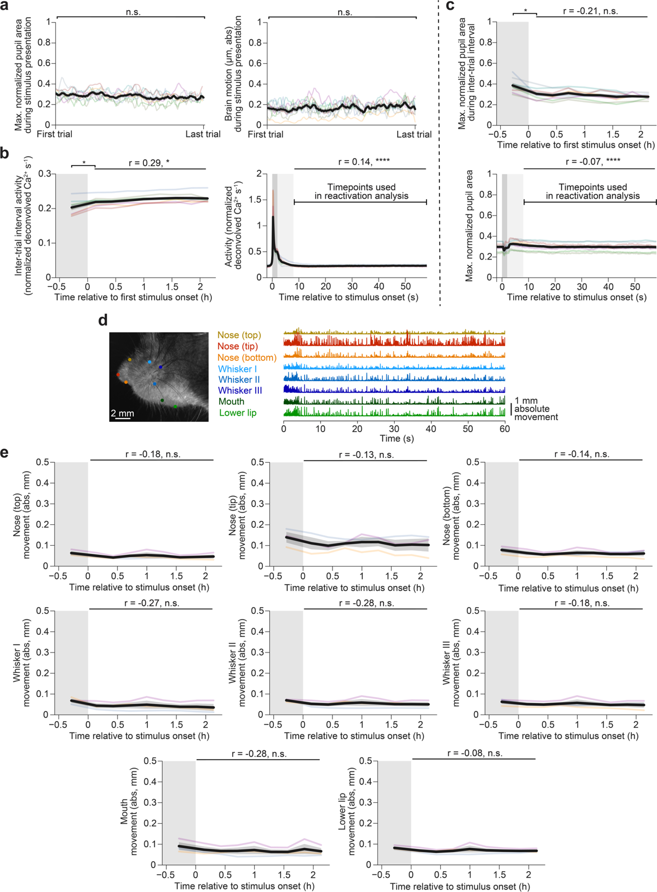
Extended Data Fig. 4 | — a, Left: peak-normalized pupil area during stimulus presentations across trials (n = 8 mice, two-tailed paired t-test, P = 0.056). Right: brain motion during stimulus presentations across trials (n = 8 mice, two-tailed paired t-test, P = 0.48). Coloured lines: individual mice. Black line: mean across mice. b, Left: Ca²⁺ activity during the baseline period before any stimulus presentation (dark shaded region) and during inter-trial intervals between stimulus presentations (n = 8 mice, two-tailed paired t-test, P = 0.016, two-tailed linear least-squares regression, P = 0.018, Holm-Bonferroni corrected). Right: Ca²⁺ activity during stimulus presentation and throughout the inter-trial interval (n = 8 mice, two-tailed linear least-squares regression, P = 1.2 × 10⁻¹⁹). Dark shaded region: stimulus presentation. Light shaded region: excluded portion of inter-trial interval. Coloured lines: individual mice. Black line: mean across mice. c, Top: peak-normalized pupil area during the baseline period before any stimulus presentation and during inter-trial intervals between stimulus presentations (n = 8 mice, two-tailed paired t-test, P = 0.019, two-tailed linear least-squares regression, P = 0.092, Holm-Bonferroni corrected). Bottom: peak-normalized pupil area during stimulus presentation and throughout the inter-trial interval (n = 8 mice, two-tailed linear least-squares regression, P = 1.7 × 10⁻⁶). Dark shaded region: stimulus presentation. Light shaded region: excluded portion of inter-trial interval. Coloured lines: individual mice. Black line: mean across mice. d, Left: example image from a recording of the mouse’s face during imaging. Each coloured dot denotes a keypoint on the face that was tracked across each session. Right: example traces of 8 tracked keypoints on the nose, whiskers, and mouth (nose top, nose tip, nose bottom, whiskers I-III, mouth, and lower lip). Traces are in units of absolute movement. e, Absolute movement of 8 tracked keypoints (nose top, nose tip, nose bottom, whiskers I-III, mouth, and lower lip) during the baseline period before any stimulus presentation and during 2.5 h of stimulus presentations (n = 3 mice, two-tailed linear least-squares regression, nose top: P = 0.39, nose tip: P = 0.54, nose bottom: P = 0.51, whisker I: P = 0.21, whisker II: P = 0.18, whisker III: P = 0.40, mouth: P = 0.19, lower lip: P = 0.70). Data are mean ± SEM. n.s.: not significant; * P < .05; **** P < .0001.

Extended Data Fig. 5 | — a, Coronal sections of visual cortex displaying virally-mediated expression of Cre-dependent jGCaMP7s in glutamatergic neurons (green, in Emx1-Cre mice) and Chrimson in parvalbumin interneurons (red, S5E2 enhancer) in 3 mice. Local injections ensured targeted expression of Chrimson throughout lateral visual cortical areas in all 3 mice. b, Left: stimulus-evoked Ca²⁺ activity during control vs. stimulus-inhibition trials (n = 3 mice, two-tailed paired t-test, P = 0.0056). Right: percent reduction in Ca²⁺ activity on stimulus-inhibition trials compared to control trials (n = 3 mice, one-sample t-test vs. 0, P = 0.0022). For stimulus-inhibition trials, we pulsed 10 mW of red light for 4 ms at 16 Hz from 1 s before stimulus onset to 1 s after stimulus offset. c, Peak-normalized pupil area during stimulus presentation and during the inter-trial interval for control vs. stimulus-inhibition trials (n = 3 mice, two-tailed paired t-test between mean of traces during the stimulus period plus the period immediately following the stimulus, P = 0.75, or during the specified inter-trial interval, P = 0.76, Holm-Bonferroni corrected). Red horizontal bar at top indicates timing of optogenetic silencing. Noise bars indicate time of visual stimulus. Grey shaded area indicates post-stimulus period excluded from reactivation analyses. d, Ca²⁺ activity during stimulus presentation and during the inter-trial interval for control vs. stimulus-inhibition trials (n = 3 mice, two-tailed paired t-test between mean of traces during the specified inter-trial interval, P = 0.19). Red horizontal bar at top indicates timing of optogenetic silencing. Noise bars indicate time of visual stimulus. Grey shaded area indicates post-stimulus period excluded from reactivation analyses. e, Reactivation rate during the inter-trial interval for all stimulus-inhibition trials that were proceeded by a control trial (n = 3 mice, two-tailed linear least-squares regression, Holm-Bonferroni corrected, control trials: P = 0.016, stimulus-inhibition trials: P = 0.38). f, Pupil size-matched reactivation rate during the baseline period before stimulus presentation and during the ITI following stimulus-inhibition trials (n = 3 mice, two-tailed paired t-test, P = 0.018). Times were selected such that the mean pupil size between the two conditions was identical (see Methods). g, Bias index of reactivation content during the inter-trial interval for all stimulus-inhibition trials that were proceeded by a control trial (n = 3 mice, two-tailed linear least-squares regression, Holm-Bonferroni corrected, control trials: P = 0.40, stimulus-inhibition trials: P = 0.66). Here, the bias index is calculated throughout as the bias in reactivation content towards the stimulus presented on the control trial (black vertical line). h, Mean reactivation rate for non-inhibition mice (n = 5 mice) across all trials and for stimulus-inhibition mice (n = 3 mice) across all trials or control (no-inhibition) trials (two-tailed unpaired t-test, Holm-Bonferroni corrected, non-inhibition mice all trials vs. stimulus-inhibition mice all trials: P = 0.11, non-inhibition mice all trials vs. stimulus-inhibition mice control trials: P = 0.019). Data are mean ± SEM. n.s.: not significant; * P < .05; ** P < .01.

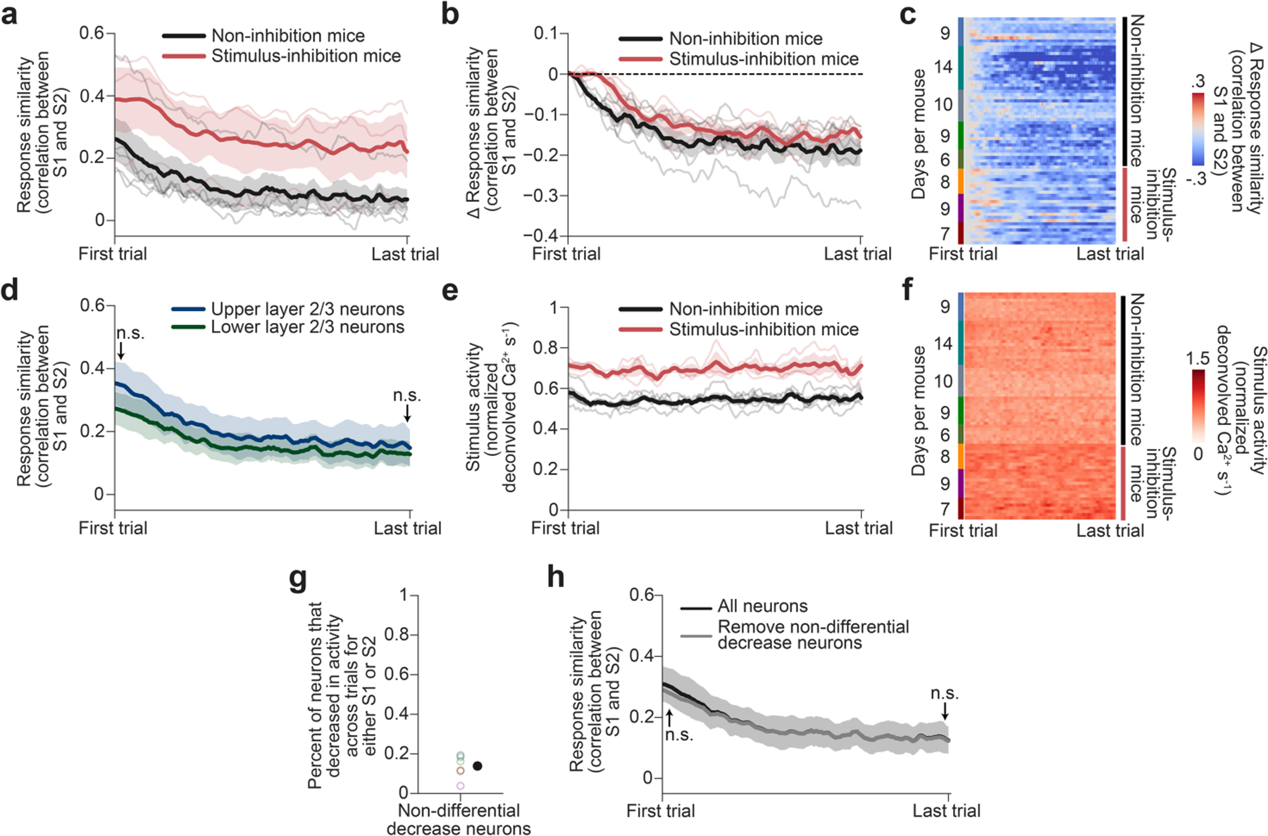
Extended Data Fig. 6 | — a, Response similarity shown separately for non-inhibition mice (n = 5 mice) and stimulus-inhibition mice (n = 3 mice; using no-inhibition control trials only). b, Change in response similarity (same as a but after subtracting the mean response similarity in first 3 trials) shown separately for non-inhibition mice (n = 5 mice) and stimulus-inhibition mice (n = 3 mice). c, Heatmap of change in response similarity shown separately for non-inhibition mice (n = 5 mice) and stimulus-inhibition mice (n = 3 mice) for all sessions. d, Response similarity using neurons located in upper layer 2/3 or lower layer 2/3 (n = 8 mice, two-tailed unpaired t-test between the mean of the first or last 3 datapoints of the two traces, Holm-Bonferroni corrected, first: P = 0.74, last: P = 0.85). e, Mean stimulus-evoked activity per trial (across all S1 and S2 trials) averaged across all stimulus-driven neurons shown separately for non-inhibition mice (n = 5 mice) and stimulus-inhibition mice (n = 3 mice; using control trials only). f, Heatmap of mean stimulus-evoked activity shown separately for non-inhibition mice (n = 5 mice) and stimulus-inhibition mice (n = 3 mice) for all sessions. g, Percent of decrease neurons that showed a similar decrease in response to both S1 and S2 (defined as a similar drop in Ca²⁺ events/second and/or a similar proportional drop in response magnitude to S1 and S2, n = 8 mice). h, Response similarity when using all neurons or when omitting non-differential decrease neurons (n = 8 mice, permutation test between the mean of the first or last 3 datapoints of the two traces, Holm-Bonferroni corrected, first: P = 0.73, last: P = 0.79). Data are mean ± SEM. n.s.: not significant.

Extended Data Fig. 7 | — a, Left: example zoom-in of the same subregion of a field of view across six days of imaging. Green, orange, purple, and red boxes highlight the same neurons tracked across all six days. Right: example neurons and masks tracked across six days of imaging, colour-matched to the neurons outlined in the left panel. b, The number of neurons tracked across all six days of imaging (n = 5 non-inhibition mice). c, Change in response similarity from the end of the previous day to the start of the next day across six days of imaging (n = 5 non-inhibition mice, two-tailed paired t-test, P = 0.42). Positive values indicate an increase in response similarity, reflecting a partial relapse in response similarity. Data are mean ± SEM. n.s.: not significant.

Extended Data Fig. 8 | — a, Mean stimulus-evoked activity across trials shown separately for non-inhibition mice (n = 5 mice) and stimulus-inhibition mice (n = 3 mice, control trials only) for no-change (left), increase (middle), or decrease (right) neuron groups. b, Numbers of neurons that are characterized as no-change, increase, or decrease neurons (n = 8 mice). c, Baseline activity before any stimulus presentation for no-change, increase, and decrease neurons (n = 8 mice, one-way ANOVA, Tukey HSD corrected, P > .05 for all tests). d, Percent of all neurons in visual region LI, POR, P, or LM that were defined as no-change, increase, or decrease neurons (n = 8 mice, one-way ANOVA, Tukey HSD corrected, P > .05 for all tests). e, Percent of all neurons in upper layer 2/3 or in lower layer 2/3 that were characterized as no-change, increase, or decrease neurons (n = 8 mice, two-tailed unpaired t-test, Holm-Bonferroni corrected, P > .05 for all tests). f, Within-group noise correlation (see Methods) of no-change, increase, or decrease neurons (n = 8 mice, one-way ANOVA, Tukey HSD corrected, P > .05 for all tests). g, Response similarity (running correlation between response patterns during neighbouring S1 and S2 trials), plotted in the same manner as the mean trace in Fig. 3g for increase neurons (left) and decrease neurons (right), but shown separately for non-inhibition mice (n = 5 mice) and stimulus-inhibition mice (n = 3 mice). h, Fraction of neurons that increase or decrease their stimulus selectivity (selectivity index: (S1_response – S2_response) / (S1_response + S2_response); see Methods) from early to late trials for no-change, increase, or decrease neurons, shown separately for non-inhibition mice (n = 5 mice) and stimulus-inhibition mice (n = 3 mice). i, Cross-correlation between high-pass filtered (see Methods) response similarity and reactivation probability traces shown separately for non-inhibition mice (n = 5 mice) and stimulus-inhibition mice (n = 3 mice). Data are mean ± SEM. n.s.: not significant.

Extended Data Fig. 9 | — a, For each trial, we projected single-trial response patterns (during S1 or S2) and stimulus-specific reactivations during the inter-trial interval (S1R or S2R) onto the axis between early and late stimulus-evoked response patterns within a session (see Fig. 4a, b for additional graphical details). Here, data from a typical example session is shown. b, Same as a but for the mean across all sessions and mice shown separately for non-inhibition mice (n = 5 mice) and stimulus-inhibition mice (n = 3 mice). c, Same as Fig. 4b but shown separately for each of the first six days of imaging per mouse, using all neurons that were tracked across the six days (n = 5 non-inhibition mice). The change in overall y-axis offset per day is not meaningful in this case since each projection uses a different projection axis estimated on each day ‘i’, i = 1–6. d, Same as Fig. 4b but using only neurons from upper layer 2/3 or from lower layer 2/3 (n = 8 mice, permutation test between the mean of the first or last 3 datapoints of the upper layer vs. lower layer traces, Holm-Bonferroni corrected, P > .05 for all tests). e, Same as Fig. 4b but after removing non-differential decrease neurons (see Extended Data Fig. 6g, n = 8 mice, permutation test between the mean of the first or last 3 datapoints of the traces generated using data from all neurons vs. from all neurons after removing non-differential decrease neurons, Holm-Bonferroni corrected, P > .05 for all tests). f, Ratio of mean activity across trials early in each session in increase (top) or decrease (bottom) neurons relative to no-change neurons during S1 presentations vs. S1R reactivation events, and during S2 presentations vs. S2R reactivation events, shown separately for non-inhibition mice (n = 5 mice) and stimulus-inhibition mice (n = 3 mice). g, Stimulus-evoked activity vs. reactivation activity, averaged across all stimulus-driven neurons (n = 8 mice). h, Difference between a neuron’s 1.3x-scaled peri-reactivation activity and its peri-stimulus activity early in each session, averaged across neurons in each group, and shown separately for non-inhibition mice (n = 5 mice) and stimulus-inhibition mice (n = 3 mice). i, Difference between a neuron’s 1.3x-scaled peri-reactivation activity and its peri-stimulus activity early in each session for S1 and S2 trials for neurons that change their stimulus preference (from early to late trials), either from being driven only by S1 to being driven only by S2 (top) or from being driven only by S2 to being driven only by S1 (bottom, n = 8 mice, two-tailed paired t-test, top: P = 3.7 × 10⁻⁴, bottom: P = 0.0034). Data are mean ± SEM. n.s.: not significant; ** P < .01; *** P < .001.

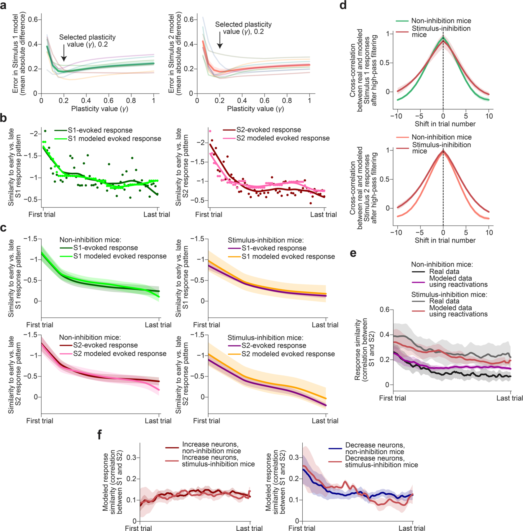
Extended Data Fig. 10 | — a, We parametrically varied the plasticity variable γ and measured the error in the modelled stimulus-evoked response patterns vs. actual stimulus-evoked response patterns (mean of the absolute difference between actual and modelled data). The value of 0.2 had the least mean error for both S1 and S2 (n = 8 mice). We used this same value for modelling all sessions and mice. This value is likely an overestimate as we do not consider plasticity that occurs during the stimulus response period. b, Comparison of projection of the actual stimulus-evoked response patterns (dark green/red dots and smoothed trace) with the modelled patterns (light green/pink dots and smoothed trace), projected onto V_s for a single session. c, Comparison of projection of the actual stimulus-evoked response patterns with the modelled patterns, projected onto V_s across all days and mice, shown separately for non-inhibition mice (n = 5 mice) and stimulus-inhibition mice (n = 3 mice). d, Cross-correlation between high-pass filtered actual and modelled projections of stimulus-evoked response patterns shown separately for non-inhibition mice (n = 5 mice) and stimulus-inhibition mice (n = 3 mice, see Methods). e, Response similarity as measured by the correlation between the mean response patterns during nearby S1 and S2 trials, plotted for actual and modelled stimulus responses, shown separately for non-inhibition mice (n = 5 mice) and stimulus-inhibition mice (n = 3 mice). f, Response similarity using modelled data, for increase or decrease neuron groups, shown separately for non-inhibition mice (n = 5 mice) and stimulus-inhibition mice (n = 3 mice). As in Fig. 3g, only decrease neurons show orthogonalization across trials, and this was evident in both sets of mice.

Supplementary Material

PeerReviewFile

NIHMS1972715-supplement-PeerReviewFile.pdf^{(7MB, pdf)}

Reporting Summary

NIHMS1972715-supplement-Reporting_Summary.pdf^{(141KB, pdf)}

Acknowledgements

We thank C. Harvey, B. McNaughton, S. Zhang, R. Essner, A. Lowet, D. Tingley, A. Sugden, J. Zaremba, M. Nguyen and the members of the Andermann laboratory for feedback; A. Sambangi for help validating AAV-S5E2-Chrimson; and K. Lensjø for advice on AAV-PHP.eb-jGCaMP7s. This project was supported by a National Defense Science and Engineering Fellowship and a Howard Hughes Medical Institute Gilliam Fellowship (to N.D.N.), NIH F32 DK112589 and Davis Family Foundation awards (to A.L.), and NIH DP2 DK105570, R01 MH12343, DP1 AT010971, a McKnight Scholar Award and a Harvard Brain Science Initiative Bipolar Disorder Seed Grant, supported by K. and L. Dauten (to M.L.A.). Icons in Figs. 1a,b,f and 2d were created using BioRender.

Footnotes

Online content

Any methods, additional references, Nature Portfolio reporting summaries, source data, extended data, supplementary information, acknowledgements, peer review information; details of author contributions and competing interests; and statements of data and code availability are available at https://doi.org/10.1038/s41586-023-06810-1.

Reporting summary

Further information on research design is available in the Nature Portfolio Reporting Summary linked to this article.

Code availability

Code is available at GitHub (https://github.com/nguyenr95/reactivation).

Competing interests The authors declare no competing interests.

Supplementary information The online version contains supplementary material available at https://doi.org/10.1038/s41586-023-06810-1.

Data availability

Processed imaging and behavioural data are available online (https://research.bidmc.harvard.edu/datashare/DataShareInfo.ASP?Submit=Display&ID=11). Raw imaging and behavioural data are available on request.

References

1.Foster DJ Replay comes of age. Annu. Rev. Neurosci 40, 581–602 (2017). [DOI] [PubMed] [Google Scholar]
2.Tambini A & Davachi L Awake reactivation of prior experiences consolidates memories and biases cognition. Trends Cogn. Sci 23, 876–890 (2019). [DOI] [PMC free article] [PubMed] [Google Scholar]
3.Failor SW, Carandini M & Harris KD Visuomotor association orthogonalizes visual cortical population codes. Preprint at bioRxiv 10.1101/2021.05.23.445338 (2022). [DOI] [Google Scholar]
4.Schoonover CE et al. Representational drift in primary olfactory cortex. Nature 594, 541–546 (2021). [DOI] [PubMed] [Google Scholar]
5.Marks TD & Goard MJ Stimulus-dependent representational drift in primary visual cortex. Nat. Commun 12, 5169 (2021). [DOI] [PMC free article] [PubMed] [Google Scholar]
6.Deitch D, Rubin A & Ziv Y Representational drift in the mouse visual cortex. Curr. Biol 31, 4327–4339 (2021). [DOI] [PubMed] [Google Scholar]
7.Clifford CW et al. Orthogonal adaptation improves orientation discrimination. Vision Res. 41, 151–159 (2001). [DOI] [PubMed] [Google Scholar]
8.Karlsson MP & Frank LM Awake replay of remote experiences in the hippocampus. Nat. Neurosci 12, 913–918 (2009). [DOI] [PMC free article] [PubMed] [Google Scholar]
9.Lee AK & Wilson MA Memory of sequential experience in the hippocampus during slow wave sleep. Neuron 36, 1183–1194 (2002). [DOI] [PubMed] [Google Scholar]
10.Nadasdy Z et al. Replay and time compression of recurring spike sequences in the hippocampus. J. Neurosci 19, 9497–9507 (1999). [DOI] [PMC free article] [PubMed] [Google Scholar]
11.Tang W et al. Hippocampal-prefrontal reactivation during learning is stronger in awake compared with sleep states. J. Neurosci 37, 11789–11805 (2017). [DOI] [PMC free article] [PubMed] [Google Scholar]
12.Carrillo-Reid L et al. Imprinting and recalling cortical ensembles. Science 353, 691–694 (2016). [DOI] [PMC free article] [PubMed] [Google Scholar]
13.Ji D & Wilson MA Coordinated memory replay in the visual cortex and hippocampus during sleep. Nat. Neurosci 10, 100–107 (2007). [DOI] [PubMed] [Google Scholar]
14.O’Neill J et al. Superficial layers of the medial entorhinal cortex replay independently of the hippocampus. Science 355, 184–188 (2017). [DOI] [PubMed] [Google Scholar]
15.Reitich-Stolero T & Paz R Affective memory rehearsal with temporal sequences in amygdala neurons. Nat. Neurosci 22, 2050–2059 (2019). [DOI] [PubMed] [Google Scholar]
16.Rothschild G, Eban E & Frank LM A cortical-hippocampal-cortical loop of information processing during memory consolidation. Nat. Neurosci 20, 251–259 (2017). [DOI] [PMC free article] [PubMed] [Google Scholar]
17.Shin JD, Tang W & Jadhav SP Dynamics of awake hippocampal-prefrontal replay for spatial learning and memory-guided decision making. Neuron 104, 1110–1125 (2019). [DOI] [PMC free article] [PubMed] [Google Scholar]
18.Sugden AU et al. Cortical reactivations of recent sensory experiences predict bidirectional network changes during learning. Nat. Neurosci 23, 981–991 (2020). [DOI] [PMC free article] [PubMed] [Google Scholar]
19.Euston DR, Tatsuno M & McNaughton BL Fast-forward playback of recent memory sequences in prefrontal cortex during sleep. Science 318, 1147–1150 (2007). [DOI] [PubMed] [Google Scholar]
20.Khodagholy D, Gelinas JN & Buzsaki G Learning-enhanced coupling between ripple oscillations in association cortices and hippocampus. Science 358, 369–372 (2017). [DOI] [PMC free article] [PubMed] [Google Scholar]
21.Lines J & Yuste R Visually evoked neuronal ensembles reactivate during sleep. Preprint at bioRxiv 10.1101/2023.04.26.538480 (2023). [DOI] [Google Scholar]
22.Chang H et al. Cortical reactivation of non-spatial and spatial memory representations coordinate with hippocampus to form a memory dialogue. Preprint at bioRxiv 10.1101/2022.12.16.520658 (2022). [DOI] [Google Scholar]
23.Eagleman SL & Dragoi V Image sequence reactivation in awake V4 networks. Proc. Natl Acad. Sci. USA 109, 19450–19455 (2012). [DOI] [PMC free article] [PubMed] [Google Scholar]
24.Genzel L et al. A consensus statement: defining terms for reactivation analysis. Philos. Trans. R. Soc. Lond. B 375, 20200001 (2020). [DOI] [PMC free article] [PubMed] [Google Scholar]
25.Swanson RA et al. Variable specificity of memory trace reactivation during hippocampal sharp wave ripples. Curr. Opin. Behav. Sci 32, 126–135 (2020). [DOI] [PMC free article] [PubMed] [Google Scholar]
26.Gupta AS et al. Hippocampal replay is not a simple function of experience. Neuron 65, 695–705 (2010). [DOI] [PMC free article] [PubMed] [Google Scholar]
27.Terada S et al. Adaptive stimulus selection for consolidation in the hippocampus. Nature 601, 240–244 (2022). [DOI] [PMC free article] [PubMed] [Google Scholar]
28.Stringer C et al. Spontaneous behaviors drive multidimensional, brainwide activity. Science 364, 255 (2019). [DOI] [PMC free article] [PubMed] [Google Scholar]
29.Cooke SF et al. Visual recognition memory, manifested as long-term habituation, requires synaptic plasticity in V1. Nat. Neurosci 18, 262–271 (2015). [DOI] [PMC free article] [PubMed] [Google Scholar]
30.Frenkel MY et al. Instructive effect of visual experience in mouse visual cortex. Neuron 51, 339–349 (2006). [DOI] [PubMed] [Google Scholar]
31.Dana H et al. High-performance calcium sensors for imaging activity in neuronal populations and microcompartments. Nat. Methods 16, 649–657 (2019). [DOI] [PubMed] [Google Scholar]
32.Gorski JA et al. Cortical excitatory neurons and glia, but not GABAergic neurons, are produced in the Emx1-expressing lineage. J. Neurosci 22, 6309–6314 (2002). [DOI] [PMC free article] [PubMed] [Google Scholar]
33.Ramesh RN et al. Intermingled ensembles in visual association cortex encode stimulus identity or predicted outcome. Neuron 100, 900–915 (2018). [DOI] [PMC free article] [PubMed] [Google Scholar]
34.Zhuang J et al. An extended retinotopic map of mouse cortex. eLife. 6, e18372 (2017). [DOI] [PMC free article] [PubMed] [Google Scholar]
35.Bradley MM et al. The pupil as a measure of emotional arousal and autonomic activation. Psychophysiology 45, 602–607 (2008). [DOI] [PMC free article] [PubMed] [Google Scholar]
36.Jeong H et al. Sensory cortical ensembles exhibit differential coupling to ripples in distinct hippocampal subregions. Curr. Biol 10.1016/j.cub.2023.10.073 (2023). [DOI] [PMC free article] [PubMed] [Google Scholar]
37.Berners-Lee A et al. Hippocampal replays appear after a single experience and incorporate greater detail with more experience. Neuron 110, 1829–1842 e5 (2022). [DOI] [PMC free article] [PubMed] [Google Scholar]
38.Gillespie AK et al. Hippocampal replay reflects specific past experiences rather than a plan for subsequent choice. Neuron 109, 3149–3163 (2021). [DOI] [PMC free article] [PubMed] [Google Scholar]
39.Singer AC & Frank LM Rewarded outcomes enhance reactivation of experience in the hippocampus. Neuron 64, 910–921 (2009). [DOI] [PMC free article] [PubMed] [Google Scholar]
40.Zutshi I & Buzsaki G Hippocampal sharp-wave ripples and their spike assembly content are regulated by the medial entorhinal cortex. Curr. Biol 33, 3648–3659 (2023). [DOI] [PMC free article] [PubMed] [Google Scholar]
41.Vormstein-Schneider D et al. Viral manipulation of functionally distinct interneurons in mice, non-human primates and humans. Nat. Neurosci 23, 1629–1636 (2020). [DOI] [PMC free article] [PubMed] [Google Scholar]
42.Schmid C et al. Passive exposure to task-relevant stimuli enhances categorization learning. eLife 12, RP88406 (2023). [DOI] [PMC free article] [PubMed] [Google Scholar]
43.McGuire KL et al. Visual association cortex links cues with conjunctions of reward and locomotor contexts. Curr. Biol 32, 1563–1576 (2022). [DOI] [PubMed] [Google Scholar]
44.Slomowitz E et al. Interplay between population firing stability and single neuron dynamics in hippocampal networks. eLife 4, e04378 (2015). [DOI] [PMC free article] [PubMed] [Google Scholar]
45.Hengen KB et al. Firing rate homeostasis in visual cortex of freely behaving rodents. Neuron 80, 335–342 (2013). [DOI] [PMC free article] [PubMed] [Google Scholar]
46.Roux L et al. Sharp wave ripples during learning stabilize the hippocampal spatial map. Nat. Neurosci 20, 845–853 (2017). [DOI] [PMC free article] [PubMed] [Google Scholar]
47.Grosmark AD et al. Reactivation predicts the consolidation of unbiased long-term cognitive maps. Nat. Neurosci 24, 1574–1585 (2021). [DOI] [PubMed] [Google Scholar]
48.van de Ven GM et al. Hippocampal offline reactivation consolidates recently formed cell assembly patterns during sharp wave-ripples. Neuron 92, 968–974 (2016). [DOI] [PMC free article] [PubMed] [Google Scholar]
49.Jun JJ et al. Fully integrated silicon probes for high-density recording of neural activity. Nature 551, 232–236 (2017). [DOI] [PMC free article] [PubMed] [Google Scholar]
50.Ego-Stengel V & Wilson MA Disruption of ripple-associated hippocampal activity during rest impairs spatial learning in the rat. Hippocampus 20, 1–10 (2010). [DOI] [PMC free article] [PubMed] [Google Scholar]
51.Jadhav SP et al. Awake hippocampal sharp-wave ripples support spatial memory. Science 336, 1454–1458 (2012). [DOI] [PMC free article] [PubMed] [Google Scholar]
52.Girardeau G et al. Selective suppression of hippocampal ripples impairs spatial memory. Nat. Neurosci 12, 1222–1223 (2009). [DOI] [PubMed] [Google Scholar]
53.Fauth MJ & van Rossum MC Self-organized reactivation maintains and reinforces memories despite synaptic turnover. eLife 8, e43717 (2019). [DOI] [PMC free article] [PubMed] [Google Scholar]
54.Mau W, Hasselmo ME and Cai DJ The brain in motion: how ensemble fluidity drives memory-updating and flexibility. eLife 9, e63550 (2020). [DOI] [PMC free article] [PubMed] [Google Scholar]
55.Hanert A et al. Sleep in humans stabilizes pattern separation performance. J. Neurosci 37, 12238–12246 (2017). [DOI] [PMC free article] [PubMed] [Google Scholar]
56.Miller JE et al. Visual stimuli recruit intrinsically generated cortical ensembles. Proc. Natl Acad. Sci. USA 111, E4053–E4061 (2014). [DOI] [PMC free article] [PubMed] [Google Scholar]
57.Vaz AP et al. Backbone spiking sequence as a basis for preplay, replay, and default states in human cortex. Nat. Commun 14, 4723 (2023). [DOI] [PMC free article] [PubMed] [Google Scholar]
58.Karlsson MP & Frank LM Network dynamics underlying the formation of sparse, informative representations in the hippocampus. J. Neurosci 28, 14271–14281 (2008). [DOI] [PMC free article] [PubMed] [Google Scholar]
59.Rolls ET The mechanisms for pattern completion and pattern separation in the hippocampus. Front. Syst. Neurosci 7, 74 (2013). [DOI] [PMC free article] [PubMed] [Google Scholar]
60.McClelland JL, McNaughton BL & O’Reilly RC Why there are complementary learning systems in the hippocampus and neocortex: insights from the successes and failures of connectionist models of learning and memory. Psychol. Rev 102, 419–457 (1995). [DOI] [PubMed] [Google Scholar]
61.Liang L et al. Retinal inputs to the thalamus are selectively gated by arousal. Curr. Biol 30, 3923–3934 (2020). [DOI] [PMC free article] [PubMed] [Google Scholar]
62.Goldey GJ et al. Removable cranial windows for long-term imaging in awake mice. Nat. Protoc 9, 2515–2538 (2014). [DOI] [PMC free article] [PubMed] [Google Scholar]
63.Wang Q & Burkhalter A Area map of mouse visual cortex. J. Comp. Neurol 502, 339–357 (2007). [DOI] [PubMed] [Google Scholar]
64.Pachitariu M et al. Suite2p: beyond 10,000 neurons with standard two-photon microscopy. Preprint at bioRxiv 10.1101/061507 (2017). [DOI] [Google Scholar]
65.Friedrich J, Zhou P & Paninski L Fast online deconvolution of calcium imaging data. PLoS Comput Biol. 13, e1005423 (2017). [DOI] [PMC free article] [PubMed] [Google Scholar]
66.Syeda A et al. Facemap: a framework for modeling neural activity based on orofacial tracking. Preprint at bioRxiv 10.1101/2022.11.03.515121 (2022). [DOI] [PMC free article] [PubMed] [Google Scholar]

Associated Data

This section collects any data citations, data availability statements, or supplementary materials included in this article.

Supplementary Materials

PeerReviewFile

NIHMS1972715-supplement-PeerReviewFile.pdf^{(7MB, pdf)}

Reporting Summary

NIHMS1972715-supplement-Reporting_Summary.pdf^{(141KB, pdf)}

Data Availability Statement

[R1] 1.Foster DJ Replay comes of age. Annu. Rev. Neurosci 40, 581–602 (2017). [DOI] [PubMed] [Google Scholar]

[R2] 2.Tambini A & Davachi L Awake reactivation of prior experiences consolidates memories and biases cognition. Trends Cogn. Sci 23, 876–890 (2019). [DOI] [PMC free article] [PubMed] [Google Scholar]

[R3] 3.Failor SW, Carandini M & Harris KD Visuomotor association orthogonalizes visual cortical population codes. Preprint at bioRxiv 10.1101/2021.05.23.445338 (2022). [DOI] [Google Scholar]

[R4] 4.Schoonover CE et al. Representational drift in primary olfactory cortex. Nature 594, 541–546 (2021). [DOI] [PubMed] [Google Scholar]

[R5] 5.Marks TD & Goard MJ Stimulus-dependent representational drift in primary visual cortex. Nat. Commun 12, 5169 (2021). [DOI] [PMC free article] [PubMed] [Google Scholar]

[R6] 6.Deitch D, Rubin A & Ziv Y Representational drift in the mouse visual cortex. Curr. Biol 31, 4327–4339 (2021). [DOI] [PubMed] [Google Scholar]

[R7] 7.Clifford CW et al. Orthogonal adaptation improves orientation discrimination. Vision Res. 41, 151–159 (2001). [DOI] [PubMed] [Google Scholar]

[R8] 8.Karlsson MP & Frank LM Awake replay of remote experiences in the hippocampus. Nat. Neurosci 12, 913–918 (2009). [DOI] [PMC free article] [PubMed] [Google Scholar]

[R9] 9.Lee AK & Wilson MA Memory of sequential experience in the hippocampus during slow wave sleep. Neuron 36, 1183–1194 (2002). [DOI] [PubMed] [Google Scholar]

[R10] 10.Nadasdy Z et al. Replay and time compression of recurring spike sequences in the hippocampus. J. Neurosci 19, 9497–9507 (1999). [DOI] [PMC free article] [PubMed] [Google Scholar]

[R11] 11.Tang W et al. Hippocampal-prefrontal reactivation during learning is stronger in awake compared with sleep states. J. Neurosci 37, 11789–11805 (2017). [DOI] [PMC free article] [PubMed] [Google Scholar]

[R12] 12.Carrillo-Reid L et al. Imprinting and recalling cortical ensembles. Science 353, 691–694 (2016). [DOI] [PMC free article] [PubMed] [Google Scholar]

[R13] 13.Ji D & Wilson MA Coordinated memory replay in the visual cortex and hippocampus during sleep. Nat. Neurosci 10, 100–107 (2007). [DOI] [PubMed] [Google Scholar]

[R14] 14.O’Neill J et al. Superficial layers of the medial entorhinal cortex replay independently of the hippocampus. Science 355, 184–188 (2017). [DOI] [PubMed] [Google Scholar]

[R15] 15.Reitich-Stolero T & Paz R Affective memory rehearsal with temporal sequences in amygdala neurons. Nat. Neurosci 22, 2050–2059 (2019). [DOI] [PubMed] [Google Scholar]

[R16] 16.Rothschild G, Eban E & Frank LM A cortical-hippocampal-cortical loop of information processing during memory consolidation. Nat. Neurosci 20, 251–259 (2017). [DOI] [PMC free article] [PubMed] [Google Scholar]

[R17] 17.Shin JD, Tang W & Jadhav SP Dynamics of awake hippocampal-prefrontal replay for spatial learning and memory-guided decision making. Neuron 104, 1110–1125 (2019). [DOI] [PMC free article] [PubMed] [Google Scholar]

[R18] 18.Sugden AU et al. Cortical reactivations of recent sensory experiences predict bidirectional network changes during learning. Nat. Neurosci 23, 981–991 (2020). [DOI] [PMC free article] [PubMed] [Google Scholar]

[R19] 19.Euston DR, Tatsuno M & McNaughton BL Fast-forward playback of recent memory sequences in prefrontal cortex during sleep. Science 318, 1147–1150 (2007). [DOI] [PubMed] [Google Scholar]

[R20] 20.Khodagholy D, Gelinas JN & Buzsaki G Learning-enhanced coupling between ripple oscillations in association cortices and hippocampus. Science 358, 369–372 (2017). [DOI] [PMC free article] [PubMed] [Google Scholar]

[R21] 21.Lines J & Yuste R Visually evoked neuronal ensembles reactivate during sleep. Preprint at bioRxiv 10.1101/2023.04.26.538480 (2023). [DOI] [Google Scholar]

[R22] 22.Chang H et al. Cortical reactivation of non-spatial and spatial memory representations coordinate with hippocampus to form a memory dialogue. Preprint at bioRxiv 10.1101/2022.12.16.520658 (2022). [DOI] [Google Scholar]

[R23] 23.Eagleman SL & Dragoi V Image sequence reactivation in awake V4 networks. Proc. Natl Acad. Sci. USA 109, 19450–19455 (2012). [DOI] [PMC free article] [PubMed] [Google Scholar]

[R24] 24.Genzel L et al. A consensus statement: defining terms for reactivation analysis. Philos. Trans. R. Soc. Lond. B 375, 20200001 (2020). [DOI] [PMC free article] [PubMed] [Google Scholar]

[R25] 25.Swanson RA et al. Variable specificity of memory trace reactivation during hippocampal sharp wave ripples. Curr. Opin. Behav. Sci 32, 126–135 (2020). [DOI] [PMC free article] [PubMed] [Google Scholar]

[R26] 26.Gupta AS et al. Hippocampal replay is not a simple function of experience. Neuron 65, 695–705 (2010). [DOI] [PMC free article] [PubMed] [Google Scholar]

[R27] 27.Terada S et al. Adaptive stimulus selection for consolidation in the hippocampus. Nature 601, 240–244 (2022). [DOI] [PMC free article] [PubMed] [Google Scholar]

[R28] 28.Stringer C et al. Spontaneous behaviors drive multidimensional, brainwide activity. Science 364, 255 (2019). [DOI] [PMC free article] [PubMed] [Google Scholar]

[R29] 29.Cooke SF et al. Visual recognition memory, manifested as long-term habituation, requires synaptic plasticity in V1. Nat. Neurosci 18, 262–271 (2015). [DOI] [PMC free article] [PubMed] [Google Scholar]

[R30] 30.Frenkel MY et al. Instructive effect of visual experience in mouse visual cortex. Neuron 51, 339–349 (2006). [DOI] [PubMed] [Google Scholar]

[R31] 31.Dana H et al. High-performance calcium sensors for imaging activity in neuronal populations and microcompartments. Nat. Methods 16, 649–657 (2019). [DOI] [PubMed] [Google Scholar]

[R32] 32.Gorski JA et al. Cortical excitatory neurons and glia, but not GABAergic neurons, are produced in the Emx1-expressing lineage. J. Neurosci 22, 6309–6314 (2002). [DOI] [PMC free article] [PubMed] [Google Scholar]

[R33] 33.Ramesh RN et al. Intermingled ensembles in visual association cortex encode stimulus identity or predicted outcome. Neuron 100, 900–915 (2018). [DOI] [PMC free article] [PubMed] [Google Scholar]

[R34] 34.Zhuang J et al. An extended retinotopic map of mouse cortex. eLife. 6, e18372 (2017). [DOI] [PMC free article] [PubMed] [Google Scholar]

[R35] 35.Bradley MM et al. The pupil as a measure of emotional arousal and autonomic activation. Psychophysiology 45, 602–607 (2008). [DOI] [PMC free article] [PubMed] [Google Scholar]

[R36] 36.Jeong H et al. Sensory cortical ensembles exhibit differential coupling to ripples in distinct hippocampal subregions. Curr. Biol 10.1016/j.cub.2023.10.073 (2023). [DOI] [PMC free article] [PubMed] [Google Scholar]

[R37] 37.Berners-Lee A et al. Hippocampal replays appear after a single experience and incorporate greater detail with more experience. Neuron 110, 1829–1842 e5 (2022). [DOI] [PMC free article] [PubMed] [Google Scholar]

[R38] 38.Gillespie AK et al. Hippocampal replay reflects specific past experiences rather than a plan for subsequent choice. Neuron 109, 3149–3163 (2021). [DOI] [PMC free article] [PubMed] [Google Scholar]

[R39] 39.Singer AC & Frank LM Rewarded outcomes enhance reactivation of experience in the hippocampus. Neuron 64, 910–921 (2009). [DOI] [PMC free article] [PubMed] [Google Scholar]

[R40] 40.Zutshi I & Buzsaki G Hippocampal sharp-wave ripples and their spike assembly content are regulated by the medial entorhinal cortex. Curr. Biol 33, 3648–3659 (2023). [DOI] [PMC free article] [PubMed] [Google Scholar]

[R41] 41.Vormstein-Schneider D et al. Viral manipulation of functionally distinct interneurons in mice, non-human primates and humans. Nat. Neurosci 23, 1629–1636 (2020). [DOI] [PMC free article] [PubMed] [Google Scholar]

[R42] 42.Schmid C et al. Passive exposure to task-relevant stimuli enhances categorization learning. eLife 12, RP88406 (2023). [DOI] [PMC free article] [PubMed] [Google Scholar]

[R43] 43.McGuire KL et al. Visual association cortex links cues with conjunctions of reward and locomotor contexts. Curr. Biol 32, 1563–1576 (2022). [DOI] [PubMed] [Google Scholar]

[R44] 44.Slomowitz E et al. Interplay between population firing stability and single neuron dynamics in hippocampal networks. eLife 4, e04378 (2015). [DOI] [PMC free article] [PubMed] [Google Scholar]

[R45] 45.Hengen KB et al. Firing rate homeostasis in visual cortex of freely behaving rodents. Neuron 80, 335–342 (2013). [DOI] [PMC free article] [PubMed] [Google Scholar]

[R46] 46.Roux L et al. Sharp wave ripples during learning stabilize the hippocampal spatial map. Nat. Neurosci 20, 845–853 (2017). [DOI] [PMC free article] [PubMed] [Google Scholar]

[R47] 47.Grosmark AD et al. Reactivation predicts the consolidation of unbiased long-term cognitive maps. Nat. Neurosci 24, 1574–1585 (2021). [DOI] [PubMed] [Google Scholar]

[R48] 48.van de Ven GM et al. Hippocampal offline reactivation consolidates recently formed cell assembly patterns during sharp wave-ripples. Neuron 92, 968–974 (2016). [DOI] [PMC free article] [PubMed] [Google Scholar]

[R49] 49.Jun JJ et al. Fully integrated silicon probes for high-density recording of neural activity. Nature 551, 232–236 (2017). [DOI] [PMC free article] [PubMed] [Google Scholar]

[R50] 50.Ego-Stengel V & Wilson MA Disruption of ripple-associated hippocampal activity during rest impairs spatial learning in the rat. Hippocampus 20, 1–10 (2010). [DOI] [PMC free article] [PubMed] [Google Scholar]

[R51] 51.Jadhav SP et al. Awake hippocampal sharp-wave ripples support spatial memory. Science 336, 1454–1458 (2012). [DOI] [PMC free article] [PubMed] [Google Scholar]

[R52] 52.Girardeau G et al. Selective suppression of hippocampal ripples impairs spatial memory. Nat. Neurosci 12, 1222–1223 (2009). [DOI] [PubMed] [Google Scholar]

[R53] 53.Fauth MJ & van Rossum MC Self-organized reactivation maintains and reinforces memories despite synaptic turnover. eLife 8, e43717 (2019). [DOI] [PMC free article] [PubMed] [Google Scholar]

[R54] 54.Mau W, Hasselmo ME and Cai DJ The brain in motion: how ensemble fluidity drives memory-updating and flexibility. eLife 9, e63550 (2020). [DOI] [PMC free article] [PubMed] [Google Scholar]

[R55] 55.Hanert A et al. Sleep in humans stabilizes pattern separation performance. J. Neurosci 37, 12238–12246 (2017). [DOI] [PMC free article] [PubMed] [Google Scholar]

[R56] 56.Miller JE et al. Visual stimuli recruit intrinsically generated cortical ensembles. Proc. Natl Acad. Sci. USA 111, E4053–E4061 (2014). [DOI] [PMC free article] [PubMed] [Google Scholar]

[R57] 57.Vaz AP et al. Backbone spiking sequence as a basis for preplay, replay, and default states in human cortex. Nat. Commun 14, 4723 (2023). [DOI] [PMC free article] [PubMed] [Google Scholar]

[R58] 58.Karlsson MP & Frank LM Network dynamics underlying the formation of sparse, informative representations in the hippocampus. J. Neurosci 28, 14271–14281 (2008). [DOI] [PMC free article] [PubMed] [Google Scholar]

[R59] 59.Rolls ET The mechanisms for pattern completion and pattern separation in the hippocampus. Front. Syst. Neurosci 7, 74 (2013). [DOI] [PMC free article] [PubMed] [Google Scholar]

[R60] 60.McClelland JL, McNaughton BL & O’Reilly RC Why there are complementary learning systems in the hippocampus and neocortex: insights from the successes and failures of connectionist models of learning and memory. Psychol. Rev 102, 419–457 (1995). [DOI] [PubMed] [Google Scholar]

[R61] 61.Liang L et al. Retinal inputs to the thalamus are selectively gated by arousal. Curr. Biol 30, 3923–3934 (2020). [DOI] [PMC free article] [PubMed] [Google Scholar]

[R62] 62.Goldey GJ et al. Removable cranial windows for long-term imaging in awake mice. Nat. Protoc 9, 2515–2538 (2014). [DOI] [PMC free article] [PubMed] [Google Scholar]

[R63] 63.Wang Q & Burkhalter A Area map of mouse visual cortex. J. Comp. Neurol 502, 339–357 (2007). [DOI] [PubMed] [Google Scholar]

[R64] 64.Pachitariu M et al. Suite2p: beyond 10,000 neurons with standard two-photon microscopy. Preprint at bioRxiv 10.1101/061507 (2017). [DOI] [Google Scholar]

[R65] 65.Friedrich J, Zhou P & Paninski L Fast online deconvolution of calcium imaging data. PLoS Comput Biol. 13, e1005423 (2017). [DOI] [PMC free article] [PubMed] [Google Scholar]

[R66] 66.Syeda A et al. Facemap: a framework for modeling neural activity based on orofacial tracking. Preprint at bioRxiv 10.1101/2022.11.03.515121 (2022). [DOI] [PMC free article] [PubMed] [Google Scholar]

PERMALINK

Cortical reactivations predict future sensory responses

Nghia D Nguyen

Andrew Lutas

Oren Amsalem

Jesseba Fernando

Andy Young-Eon Ahn

Richard Hakim

Josselyn Vergara

Justin McMahon

Jordane Dimidschstein

Bernardo L Sabatini

Mark L Andermann

Abstract

Distributed reactivations across the cortex

Fig. 1 |. Distributed stimulus reactivations in the lateral visual cortex during quiet waking.

Rates of reactivations gradually decay

Fig. 2 |. Cortical responses to stimuli drive subsequent reactivations.

Fig. 3 |. Progressive separation of stimulus response patterns correlates with reactivation rate.

Local silencing of stimulus responses

Reactivations track orthogonalization

Reactivations predict future responses

Fig. 4 |. Reactivations predict representational drift.

Modelling future stimulus responses

Discussion

Methods

Data reporting

Mice

Behavioural training

Surgical procedures

Retinotopy

Two-photon calcium imaging

Image processing and source extraction

Face and pupil tracking

Concurrent two-photon imaging of the visual cortex and hippocampal CA1 LFP recordings

Defining early and late trials in non-inhibition and stimulus-inhibition mice

Stimulus-driven neurons

Classifying stimulus reactivations

Shuffle analyses involving the stimulus reactivation classifier

Quantifying reactivation location

Quantifying reactivation rate and bias

Classifying stimulus reactivations using subsets of neurons

Optogenetic inhibition

Response metric

Defining the increase, decrease and no-change groups of neurons

Cross-correlation analysis

Noise correlation analysis

High-pass filtering

Tracking neurons across days using ROICaT

Vector analysis

Scaling reactivation responses

Modelling stimulus responses using reactivations

Data analysis

Extended Data

Extended Data Fig. 1 |. Classifying stimulus-specific reactivations.

Extended Data Fig. 2 |. Characterizing stimulus reactivations.

Extended Data Fig. 3 |. Reactivation rate and bias effects are consistent across sessions and correlate with stimulus novelty and pupil-indexed arousal.

Extended Data Fig. 4 |. Physical correlates of arousal remain constant throughout the session.

Extended Data Fig. 5 |. Characterizing the effects of peri-stimulus inhibition.

Extended Data Fig. 6 |. Compared to non-inhibition mice, stimulus-inhibition mice exhibit similar stimulus response orthogonalization but higher response magnitudes during control trials.

Extended Data Fig. 7 |. Tracking the same neurons across days.

Extended Data Fig. 8 |. Characterization of no-change, increase, and decrease neurons.

Extended Data Fig. 9 |. Stimulus reactivations consistently predict future stimulus responses.

Extended Data Fig. 10 |. Modelling future stimulus responses using only stimulus reactivations.

Supplementary Material

Acknowledgements

Footnotes

Data availability

References

Associated Data

Supplementary Materials

Data Availability Statement

ACTIONS

PERMALINK

RESOURCES

Similar articles

Cited by other articles

Links to NCBI Databases