Ecological inference for infectious disease data, with application to vaccination strategies

Abstract

Disease surveillance systems provide a rich source of data regarding infectious diseases, aggregated across geographical regions. The analysis of such ecological data is fraught with difficulties, and, unless care and suitable data summaries are available, will lead to biased estimates of individual-level parameters. We consider using surveillance data to study the impacts of vaccination. To catalog the problems of ecological inference, we start with an individual-level model, which contains familiar parameters, and derive an ecologically consistent model for infectious diseases in partially vaccinated populations. We compare with other popular model classes and highlight deficiencies. We explore the properties of the new model through simulation and demonstrate that, under standard assumptions, the ecological model provides less biased estimates. We then fit the new model to data collected on measles outbreaks in Germany from 2005–2007.

1 |. INTRODUCTION

A wide range of diseases are monitored at the local, state, and national levels using disease surveillance systems designed to assess the current disease burden or to detect emerging outbreaks. Although there are a variety of approaches to surveillance, ranging from daily collection of de-identified electronic medical records to mandatory reporting of certain notifiable diseases, the resulting data typically captures information for large populations over time. For this reason, disease surveillance systems are frequently a primary source of information for public health researchers and officials who use such data to design and deploy effective interventions. While this approach is economical, cases are typically aggregated in space, time, or both, and the information regarding any single case is limited.

This aggregation can present challenges when studying the spread of infectious disease. In the social sciences and noninfectious disease epidemiology, aggregated data is often analyzed with established disease mapping approaches such as ecological regression. However, the risk of drawing erroneous individual-level conclusions from group-level data has been well characterized.^1–6 This phenomenon is referred to as ecological bias and can arise when the form of the risk model changes under aggregation. When the model for the individual-level risk of disease is a nonlinear function of the exposure, as is typically the case for infectious disease models, the form of the marginal aggregate risk model changes as a result of the within-group variability of the exposure that is not accounted for in the group-level model.⁷

In the infectious disease setting, ecological regression approaches are typically not considered since they do not leverage known dependencies. For aggregated infectious disease data, there are two common approaches in the literature: the time series SIR (TSIR) model⁸ and the epidemic-endemic framework.^9–15 Under the TSIR approach, the number of susceptible and infected individuals are modeled independently without recourse to a development from the individual level. The epidemic-endemic framework is motivated by spatial branching processes and is closely related to standard SIR and multivariate TSIR models.¹⁶ Meanwhile, these epidemic-endemic models are easily fit in standard software via the surveillance package in the R programming environment.¹⁴ A recent review compares and contrasts the two classes of models.¹⁷ For both approaches to modeling aggregated infectious disease data, the risks of infections are nonlinear and, thus, inference is susceptible to ecological bias. However, there has been little discussion of ecological bias for aggregate infectious disease models.¹⁸ In particular, the ecological aspects of the epidemic-endemic model have not been investigated.

In this manuscript, we consider using aggregated surveillance data to study the impact of vaccination on infectious disease transmission. To avoid ecological bias, we start with an individual-level infectious disease model that includes vaccination and derive an ecologically consistent infectious disease model for a partially vaccinated populations. This ecological vaccine model is easily fit and provides estimates of familiar epidemiological parameters. The remainder of this paper is organized as follows. In Section 2, we motivate the aim of this paper and introduce some notation and preliminary concepts. In Section 3, we develop an ecologically consistent vaccine model under two models of vaccine action; we present simulations to better understand the behavior of the ecological vaccine model in Section 4; and fit the ecological vaccine model to measles data from Germany in Section 5. Final comments appear in Section 6.

2 |. MOTIVATION AND NOTATION

In surveillance data, new cases are commonly reported in discrete time and space. It is common to use time steps relative to the disease of interest, meaning that we are assuming the sum of incubation and infectious times is approximately that of the observation times. For example, for measles, the data are often aggregated over 2-week periods. We denote the number of cases and the population size for area $i$ and time $t$ by $Y_{it}$ and $N_{it}$. Let $S_{it}$ denote the number of susceptible individuals and $x_{it}$ the proportion of vaccinated individuals in area $i$ and time $t$. Area- and time-specific covariates other than vaccination coverage are denoted $z_{it}$.

Recently, the epidemic-endemic model was derived via aggregation of an individual-level model, and the framework was extended to handle a stratified population.¹⁵ We briefly review this derivation before discussing how the epidemic-endemic models are typically applied when considering vaccination. We use ${\mathit{\lambda }}_{it}^{†}$ to denote the generic force of infection, or the risk of an individual who was susceptible at time $t-1$, becoming infected by time $t$ in area $i$.¹⁹ Assuming a constant hazard of infection between time steps, the probability of a susceptible individual in area $i$ and time $t-1$ becoming infected by time $t$ is determined by the hazard rate ${\mathit{\lambda }}_{it}^{†}$, implying the following individual-level model: Pr(infection in $(t-1,t]\mid$ no infection by $t-1$, area $i)=1-e^{-{\mathit{\lambda }}_{it}^{†}}$. A Reed-Frost chain binomial SIR model is implied if we additionally assume that the time until infection is independent for all susceptible individuals¹⁹; hence, the number of new infectives in area $i$ at time $t$ can be modeled as $Y_{it}\mid {\mathit{\lambda }}_{it}^{†}\sim \text{Binomial}\left(S_{i,t-1},1-e^{-{\mathit{\lambda }}_{it}^{†}}\right)$. When ${\mathit{\lambda }}_{it}^{†}$ is small, the Taylor expansion, $1-\exp \left(-{\mathit{\lambda }}_{it}^{†}\right)\approx {\mathit{\lambda }}_{it}^{†}$, simplifies the form of the probability of infection. When the number of susceptibles, $S_{i,t-1}$ is large and the probability of infection is small, the binomial distribution can be approximated by a Poisson distribution so that $Y_{it}\mid {\mu }_{it}\sim \text{Poisson}\left({\mu }_{it}\right)$, where ${\mu }_{it}=S_{i,t-1}{\mathit{\lambda }}_{it}^{†}$. When the number of new infections is small and the population is large, the number of susceptibles can be approximated by the initial number of susceptibles, $S_{it}\approx N_i$.

In the infectious disease setting, there are typically multiple sources of infection. For example, a susceptible may become infected from an infective in their own area, another area, or from an environmental reservoir or infective external to the study region. Typically, the epidemic-endemic framework decomposes the force of infection into three components: autoregressive (AR), neighborhood (NE), and endemic (EN), where the endemic component includes all other sources of infection.⁹ For simplicity, here, we consider the AR and EN components only (though the discussion holds if neighborhood terms are included also). Considering a competing risk framework, we can write ${\mathit{\lambda }}_{it}^{†}={\mathit{\lambda }}_{it}^{\text{AR}†}+{\mathit{\lambda }}_{it}^{\text{EN}†}$, where ${\mathit{\lambda }}_{it}^{\text{AR}†}$ and ${\mathit{\lambda }}_{it}^{\text{EN}†}$ are generic forms of the component-specific risks. A frequency dependent transmission model implies ${\mathit{\lambda }}_{it}^{\text{AR}†}={\mathit{\lambda }}_{it}^{\text{AR}}{y}_{i,t-1}/N_i$.¹⁵ Then, assuming rare events and $S_{it}\approx N_i$ we obtain a general form of the epidemic-endemic model, with $Y_{it}\mid {\mu }_{it}\sim \text{Poisson}\left({\mu }_{it}\right)$, where

$${\mu }_{it}=S_{i,t-1}{\mathit{\lambda }}_{it}^{†}=\underset{\text{Autoregressive}}{\underbrace{{\mathit{\lambda }}_{it}^{\text{AR}}{y}_{i,t-1}}}+\underset{\text{Endemic}}{\underbrace{{\mathit{\lambda }}_{it}^{\text{EN}}{N}_i}}.$$ (1)

The autoregressive component accounts for the disease risk from infectives in the previous time period and in the same area. The endemic component describes the additional risk from environmental reservoirs that contribute to the risk of infection or other sources of infection not already accounted for by the other component(s). The parameters ${\mathit{\lambda }}_{it}^{\text{AR}}$ and ${\mathit{\lambda }}_{it}^{\text{EN}}$ are rates and determine the relative contributions of cases from the respective sources, though are not directly comparable.

The epidemic-endemic framework typically models the number of cases in area $i$ and time $t$ with a negative binomial distribution with mean ${\mathit{\lambda }}_{it}^{†}$.¹⁴ For simplicity, we model overdispersion via a Poisson distribution with log-normal random effects, with the mean decomposed as in Equation (1). Each component can be modeled with a log-linear model to include covariates as well as fixed and random effects. For example, the autoregressive component may take the form

$$\log {\mathit{\lambda }}_{it}^{\text{AR}}={\alpha }_{\text{AR}}+a_i+{\mathit{\beta }}^{\text{AR}}{z}_{it},$$ (2)

where ${\alpha }_{\text{AR}}$ is a log-risk intercept, $a_i$ are area-specific fixed (or random) effects, $z_{it}$ are area- and time-specific covariates, and $\exp \left({\mathit{\beta }}^{\text{AR}}\right)$ are the associated covariate relative risks. The endemic component can be modeled in a similar fashion to the above AR component. Seasonality can be included in either component of the model by adding to the log-risk, a term of the form, ${\sum }_{s=1}^S\left[{\gamma }_s\sin \left({\mathit{\omega }}_{s}t\right)+{\delta }_s\cos \left({\mathit{\omega }}_{s}t\right)\right]$, where $S$ is the number of pairs of sines and cosines to include and ${\mathit{\omega }}_s$ are Fourier frequencies. For biweekly data, ${\mathit{\omega }}_s=2\pi s/26$. In practice, seasonal terms have been included in only the endemic component.^12–14

In the surveillance package, parameter estimates are quickly obtained for the epidemic-endemic models via penalized maximum likelihood estimation.¹⁴ While epidemic-endemic models can be used for prediction, they are more often used to smooth observed counts, in which case, parameter interpretation is not done extensively. Within the epidemic-endemic framework, there has been no discussion of the ecological bias implications of the use of loglinear models of the form (2). Appendix A shows the inconsistency between the individual and ecological models in some simple situations, using this loglinear model, and simulations in Section 4.2 provide numerical examples of ecological bias in this setting.

In the context of studying vaccination on disease spread, there are two analyses that use the epidemic-endemic framework to model measles in Germany that include vaccination coverage.^12,14 Both analyses consider multiple ways of incorporating vaccination coverage into the mean model and use AIC to select a final model. However, the analyses of separate data sets produced different models for measles in Germany. One analysis included vaccination coverage in only the autoregressive component, whereas the other included it in is only the endemic component. For example, the model $Y_{it}\mid {\mu }_{it}\sim \text{Poisson}\left({\mu }_{it}\right)$ included vaccination coverage in the endemic component, with

$${\mu }_{it}={\mathit{\lambda }}_{it}^{\text{AR}}{y}_{i,t-1}+{\left(1-x_i\right)}^{{\alpha }_1}{\mathit{\lambda }}_{it}^{\text{EN}}{N}_{it}/N,$$ (3)

where $x_i$ is the proportion of vaccinated individuals in area $i$.

While this approach may lead to models that fit the data well, it fails to account for the scientific context of how vaccination affects susceptibility. In (3), if the proportion of unvaccinated individuals, $\left(1-x_i\right)$ is thought of as a proxy for the number of susceptible individuals in the population, then the parameter associated with the vaccination coverage, ${\alpha }_1$ can be thought of as a flexibility parameter to improve model fit.¹² Moreover, the interpretation of the parameter associated with vaccination coverage can be cumbersome or nonintuitive and the parameters may not be comparable across analyses. For example, the interpretation from (3) is that the expected multiplicative change in endemic incidence associated with a doubling of the proportion of susceptible individuals in area $i$ is estimated to be $2^{{\widehat{\alpha }}_1}$.¹⁴

Alternatively, it is common to account for vaccination in applications of the TSIR framework by augmenting the susceptibles model to account for vaccination coverage. For example, in the context of modeling hand, foot and mouth disease in China, the basic accounting equation for susceptibles, the number of new births is reduced by the vaccination coverage, which is assumed known and vaccine effect is not estimated.²⁰ As these examples demonstrate, current approaches to modeling aggregate data may be inappropriate when the goal is to study the covariate effects on disease spread. When the interest is to study the effects of vaccination for an imperfect vaccine, the resulting models lack familiar parameter interpretation and primarily focus on model fit.

Before proceeding, we take a moment to introduce a key parameter for quantifying infectious diseases that is regularly used in practice. The basic reproductive number, represented by $R_0$, is defined as the average number of individuals a typical infectious individual would infect in a completely susceptible population.²¹ When a portion of the population is immune, either because of vaccination or previous infection, the average number of new infections caused by a single infectious is called the effective reproductive number, represented by $R$. In our setting, where $x$ is the proportion of the population that is immune to infection, either through natural infection or vaccination, $R=(1-x)R_0$. For both $R_0$ and $R$, values less than 1 imply that major outbreaks can be avoided.

3 |. ECOLOGICAL VACCINE MODEL DEVELOPMENT

3.1 |. Introduction

With inference as a primary goal, we now develop an aggregate infectious disease model with vaccination for inference. For clarity, we develop the ecological model in a single area and with a generic force of infection, although as we show in Section 5, extensions to multiple areas and more complex forms of risk can be made. We further assume that the vaccine only affects an individual’s susceptibility to infection (and not infectiousness or disease progression) and that vaccination provides lifetime immunity. We let $\varphi$ be the reduction in a vaccine recipient’s risk of infection (the vaccine effect) after vaccination and assume a constant vaccine coverage denoted by $x$. We subscript the number of susceptibles, cases, and force of infections with $v$ and $u$ to indicate vaccinated and unvaccinated. Hence, $Y_{ut}$ and $Y_{vt}$ are the total number of unvaccinated and vaccinated infectives at time $t$, such that $Y_t=Y_{ut}+Y_{vt}$. We assume that vaccination is administered in a totally susceptible population, so that, at $t$ = 0, the number of unvaccinated susceptible individuals is $S_{u0}=(1-x)N$.

To properly model the effects of vaccination, at the population level, it is important to consider how the vaccine reduces an individual’s risk of infection. We consider aggregate models for two modes of vaccine action: leaky and all-or-none. Leaky vaccines are assumed to reduce the risk of infection by a constant proportion for all vaccinated individuals; in contrast, all-or-none vaccines provide full protection from infection to vaccinated individuals when successful but fail to provide protection with some probability.¹⁹ In other words, leaky vaccines reduce the per-exposure risk of infection, whereas an all-or-none vaccine’s protection is independent of the number of contacts made. In reality, a given vaccine may not fall squarely into one of these two categories, but we use these two different models to explore these extremes. In the subsequent sections, we show that, regardless of the assumed mode of vaccine action, there is a common ecologically consistent model that can be fit to aggregate data.

3.2 |. All-or-none vaccine ecological model

For an all-or-none vaccine, it is assumed that the vaccine fails with probability $(1-\varphi )$ and offers no partial protection in this case.¹⁹ This implies that the number of susceptible individuals who were vaccinated is $S_{v0}(\varphi )=(1-\varphi )xN$, and ${\mathit{\lambda }}_{vt}={\mathit{\lambda }}_{ut}={\mathit{\lambda }}_t^{†}$ is the common risk of infection. We denote the number of susceptibles at time $t$ by $S_t(\varphi )$ to emphasize that the number of susceptibles is a function of the vaccine effect. At time $t$ = 0, the number of susceptibles at time $S_0(\varphi )=S_{u0}(\varphi )+S_{v0}(\varphi )=(1-x)N+(1-\varphi )xN=(1-\varphi x)N$. The number of new infections at time $t+1$ can be modeled as

$$Y_{t+1}\mid {\mathit{\lambda }}_t^{†}\sim \text{Binomial}\left(S_t(\varphi ),1-\exp \left(-{\mathit{\lambda }}_t^{†}\right)\right),$$ (4)

where $S_t(\varphi )=S_{t-1}(\varphi )-Y_t$. In the rare disease setting, the binomial can be approximated by a Poisson and, when ${\mathit{\lambda }}_t^{†}$ is small, a Taylor expansion approximates $1-\exp \left(-{\mathit{\lambda }}_t^{†}\right)\approx {\mathit{\lambda }}_t^{†}$ so that $Y_{t+1}\mid {\mathit{\lambda }}_t^{†}\sim \text{Poisson}\left(S_t(\varphi ){\mathit{\lambda }}_t^{†}\right)$, where $S_t(\varphi )=(1-\varphi x)N-{\sum }_{k=1}^t{Y}_k$. When the susceptible population is sufficiently large, and the number of cases is small, the number of susceptibles is effectively constant and can be approximated by $S_t(\varphi )\approx (1-\varphi x)N$. The ecological model in (4) becomes

$$Y_{t+1}\mid {\mathit{\lambda }}_t^{†}\sim \text{Poisson}\left({\mathit{\lambda }}_t^{†}(1-\varphi x)N\right),$$ (5)

when the approximations are valid. In Section 4.1, we consider the conditions under which these modeling assumptions are reasonable.

3.3 |. Leaky vaccine ecological model

Under the leaky vaccine model, vaccinated individuals are still susceptible to infection, and therefore, $S_{u0}=(1-x)N$ and $S_{v0}=xN$. Additionally, the leaky vaccine implies that we can write the risk of infection for the vaccinated as a function of that in the unvaccinated population and the vaccine effect

$${\mathit{\lambda }}_{vt}^{†}=(1-\varphi ){\mathit{\lambda }}_{ut}^{†}.$$ (6)

Then, the number of new infections at time $t+1$ can be modeled as

$$Y_{u,t+1}\mid {\mathit{\lambda }}_{ut}^{†}\sim \text{Binomial}\left(S_{ut},1-\exp \left(-{\mathit{\lambda }}_{ut}^{†}\right)\right),$$ (7)

$$Y_{v,t+1}\mid {\mathit{\lambda }}_{vt}^{†}\sim \text{Binomial}\left(S_{vt},1-\exp \left(-{\mathit{\lambda }}_{vt}^{†}\right)\right),$$ (8)

where ${\mathit{\lambda }}_{ut}^{†}$ is the risk of infection for an unvaccinated susceptible at time $t$, and ${\mathit{\lambda }}_{vt}^{†}$ is defined in (6); the number of susceptibles at time $t+1$ are

$$S_{u,t+1}=S_{u,t}-Y_{u,t+1}\text{and}{S}_{v,t+1}=S_{v,t}-Y_{v,t+1}.$$

The resulting aggregate model is a convolution of binomials, where

$$\mathrm{Pr}\left(Y_t=y\mid {\mathit{\lambda }}_{ut}^{†},{\mathit{\lambda }}_{vt}^{†}\right)=\sum _{z=0}^y\mathrm{Pr}\left(Y_{ut}=z\mid {\mathit{\lambda }}_{ut}^{†}\right)\mathrm{Pr}\left(Y_{vt}=y-z\mid {\mathit{\lambda }}_{vt}^{†}\right).$$ (9)

When the susceptible populations or disease counts are large, this aggregate model will be computationally expensive and practically intractable. When the risks of infection are small, the Taylor approximation simplifies the probability of infection in Equations (7) and (8). Moreover, when infections are rare, the binomial distributions can be approximated by Poisson’s. Hence, when risk of infection is small for both the unvaccinated and vaccinated populations, the number of new infections in each group is approximately

$$Y_{u,t+1}\mid {\mathit{\lambda }}_{ut}^{†}\sim \text{Poisson}\left(S_{ut}{\mathit{\lambda }}_{ut}^{†}\right),$$ (10)

$$Y_{v,t+1}\mid {\mathit{\lambda }}_{ut}^{†},\varphi \sim \text{Poisson}\left(S_{vt}(1-\varphi ){\mathit{\lambda }}_{ut}^{†}\right).$$ (11)

The resulting aggregate model, when the risk is small for both vaccinated and unvaccinated groups is

$$Y_{t+1}\mid {\mathit{\lambda }}_{ut}^{†},\varphi \sim \text{Poisson}\left(\left(S_{ut}+S_{vt}(1-\varphi )\right){\mathit{\lambda }}_{ut}^{†}\right).$$ (12)

Compared to the convolution model of (9), this likelihood is more tractable in large populations with few cases. However, this model still requires knowing the number of susceptibles by vaccination status, which is typically not known or easily approximated. If it is reasonable to assume that the number of infectives is negligible when compared to the size of the susceptible pool, ie, $S_{ut}\approx S_{u0}$ and $S_{vt}\approx S_{v0}$, the ecological model for a partially vaccinated population is approximately

$$Y_{t+1}\mid {\mathit{\lambda }}_{ut}^{†},\varphi \sim \text{Poisson}\left({\mathit{\lambda }}_{ut}^{†}(1-\varphi x)N\right),$$ (13)

which is identical to the ecological model derived assuming an all-or-none vaccine given in Equation (5).

3.4 |. Comments on the ecological vaccine model

We summarize the development of the ecological vaccine model starting from the all-or-none and leaky vaccine assumptions, as well as the simplifying assumptions that result in the ecological vaccine model in Table 1.

TABLE 1.

Summary of the all-or-none and leaky vaccine models and the assumptions for the ecological vaccine model. $N$ is the total population; $x$ denotes the proportion of the population vaccinated (assumed constant over time); $\varphi$ is the vaccine effect on susceptibility; $S_{ut}$ and $S_{vt}$ denote the number of unvaccinated and vaccinated susceptibles at time $t$; $Y_{ut}$ and $Y_{vt}$ denote new cases in time $t$ among unvaccinated and vaccinated; and ${\mathit{\lambda }}_t^{†}$ is a generic force of infection

	All-or-none	Leaky
Initial susceptible population
	$S_{u0}(\varphi )=(1-x)N$	$S_{u0}=(1-x)N$
	$S_{v0}(\varphi )=(1-\varphi )xN$	$S_{y0}=xN$
Force of infection
	${\mathit{\lambda }}_{ut}^{†}={\mathit{\lambda }}_t^{†}$	${\mathit{\lambda }}_{ut}^{†}={\mathit{\lambda }}_t^{†}$
	${\mathit{\lambda }}_{vt}^{†}={\mathit{\lambda }}_t^{†}$	${\mathit{\lambda }}_{vt}^{†}=(1-\varphi ){\mathit{\lambda }}_t^{†}$
Progression
$Y_{u,t+1}\mid {\mathit{\lambda }}_{ut}^{†}$	$\text{Bin}\left(S_{ut}(\varphi ),1-e^{-{\mathit{\lambda }}_t^{†}}\right)$	$\text{Bin}\left(S_{ut},1-e^{-{\mathit{\lambda }}_t^{†}}\right)$
$Y_{v,t+1}\mid {\mathit{\lambda }}_{vt}^{†}$	$\text{Bin}\left(S_{vt}(\varphi ),1-e^{-{\mathit{\lambda }}_t^{†}}\right)$	$\text{Bin}\left(S_{vt},1-e^{-(1-\varphi ){\mathit{\lambda }}_t^{†}}\right)$
Implied aggregate model
$Y_{t+1}\mid {\mathit{\lambda }}_t^{†}$	$\text{Bin}\left(S_t(\varphi ),1-e^{-{\mathit{\lambda }}_t^{†}}\right)$	Convolution of binomials
Simplifying assumptions
Poisson's approximate binomials
	$\text{Poi}\left(S_t(\varphi )\left(1-e^{-{\mathit{\lambda }}_t^{†}}\right)\right)$	$\text{Poi}\left(S_{ut}\left(1-e^{-{\mathit{\lambda }}_t^{†}}\right)+S_{vt}\left(1-e^{-(1-\varphi ){\mathit{\lambda }}_t^{†}}\right)\right)$
Taylor approximation
	$\text{Poi}\left(S_t(\varphi ){\mathit{\lambda }}_t^{†}\right)$	$\text{Poi}\left(\left(S_{ut}+(1-\varphi )S_{vt}\right){\mathit{\lambda }}_t^{†}\right)$
Negligible number of infections
	$S_t(\varphi )\approx (1-\varphi x)N$	$S_{ut}\approx (1-x)N,S_{vt}\approx xN$
Ecological vaccine model
$Y_{t+1}\mid {\mathit{\lambda }}_t^{†},\varphi \sim \text{Poisson}\left({\mathit{\lambda }}_t^{†}(1-\varphi x)N\right)$

Both the all-or-none and leaky vaccine models can be approximated by the ecological vaccine model when the following simplifying assumptions can be made:

1. Poisson approximation to the binomial distribution;

2. force of infection approximation: $1-e^{-{\mathit{\lambda }}_t^{†}}\approx {\mathit{\lambda }}_t^{†}\text{;}$

3. negligible number of infections: $S_{ut}\approx S_{u0}$ for unvaccinated individuals, and $S_{vt}\approx S_{v0}$ for vaccinated individuals. Note that the number of susceptibles may also be a function of the vaccine effect.

This list of assumptions helps illuminate when the ecological vaccine model we have developed is appropriate to use. The fact that, when aggregated, both vaccine models can be approximated by the same model suggests that, with aggregated data, there is not sufficient information to tease apart the mechanism of vaccine protection. In fact, in Appendix B, we derive the ecological vaccine model assuming the vaccine that has both leaky and all-or-none effects and show that the specific vaccine effects are not identifiable with the ecological vaccine model.

4 |. SIMULATIONS

4.1 |. Assessing the simplifying assumptions in the absence of vaccination

We first assess the conditions under which these simplifying assumptions are appropriate in the absence of vaccination via simulation. Each simulated epidemic starts with a single infected individual in an otherwise susceptible population of N = 100 000; in other words, let $Y_0=1$ and $S_0=N-Y_0$. Moreover, the number of cases over the course of a given epidemic is simulated as follows:

$$Y_{t+1}\mid {\mathit{\lambda }}_t^{†},y_t\sim \text{Binomial}\left(S_t,1-e^{-{\mathit{\lambda }}_t^{†}}\right)\text{,}$$

$${\mathit{\lambda }}_t^{†}=e^{{\alpha }_{\text{AR}}}{y}_t/N+e^{{\alpha }_{\text{EN}}}\text{,}$$

$$S_t=N-\sum _{k=0}^t{y}_k.$$

We simulate epidemics for high, medium, and low values of $R_0$, which correspond to ${\alpha }_{\text{AR}}$ = log(2.5), log(1), or log(0.85), and fix ${\alpha }_{\text{EN}}$ = −10. To increase variability in the initial number of cases in each simulated epidemic, we discard observations from $t$ = 0, …, 4 and simulate the equivalent of 3 years of weekly data starting from $t$ = 5. We simulate 250 epidemics for each of the three simulation scenarios. For each simulated epidemic, we fit models from all possible combinations of the three simplifying assumptions summarized in Section 3.4 (and Table 1) and compare the maximum likelihood estimates (MLEs) obtained via numerical optimization. Specifically, we fit the following:

1. $Y_{t+1}\mid {\mathit{\lambda }}_t^{†}\sim \text{Binomial}\left(S_t,1-e^{-{\mathit{\lambda }}_t^{†}}\right)\text{;}$

2. $Y_{t+1}\mid {\mathit{\lambda }}_t^{†}\sim \text{Binomial}\left(N,1-e^{-{\mathit{\lambda }}_t^{†}}\right)\text{;}$

3. $Y_{t+1}\mid {\mathit{\lambda }}_t^{†}\sim \text{Binomial}\left(S_t,{\mathit{\lambda }}_t^{†}\right)\text{;}$

4. $Y_{t+1}\mid {\mathit{\lambda }}_t^{†}\sim \text{Binomial}\left(N,{\mathit{\lambda }}_t^{†}\right)\text{;}$

5. $Y_{t+1}\mid {\mathit{\lambda }}_t^{†}\sim \text{Poisson}\left(S_t\left(1-e^{-{\mathit{\lambda }}_t^{†}}\right)\right)\text{;}$

6. $Y_{t+1}\mid {\mathit{\lambda }}_t^{†}\sim \text{Poisson}\left(N\left(1-e^{-{\mathit{\lambda }}_t^{†}}\right)\right)\text{;}$

7. $Y_{t+1}\mid {\mathit{\lambda }}_t^{†}\sim \text{Poisson}\left(S_t{\mathit{\lambda }}_t^{†}\right)\text{;}$

8. $Y_{t+1}\mid {\mathit{\lambda }}_t^{†}\sim \text{Poisson}\left(N{\mathit{\lambda }}_t^{†}\right)$.

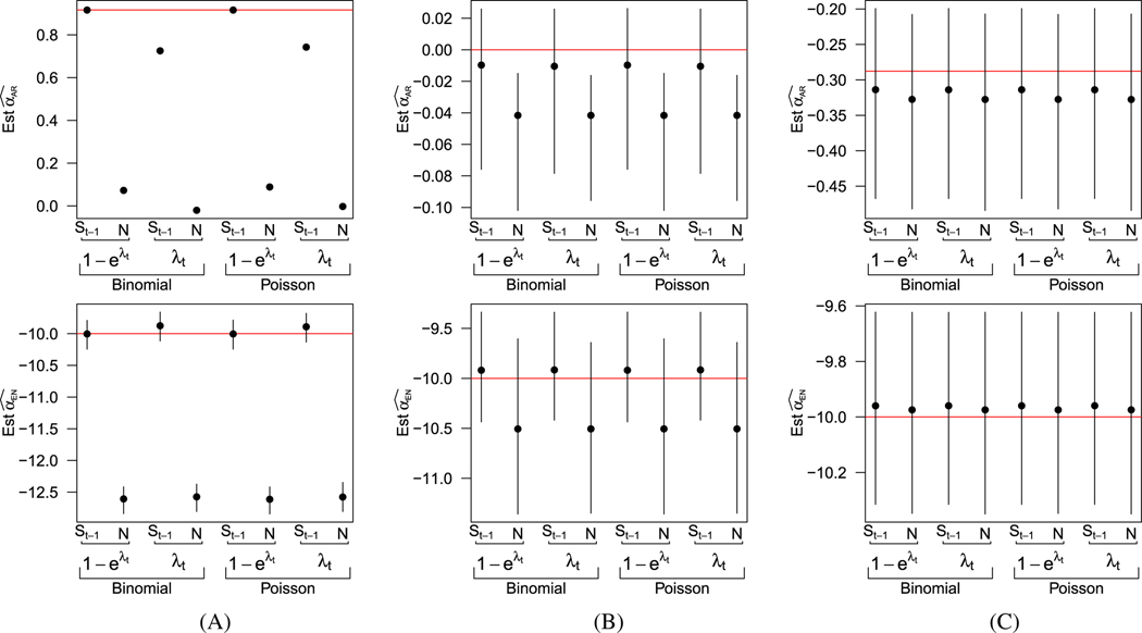
For all eight models, the force of infection is modeled as ${\mathit{\lambda }}_t^{†}=e^{{\alpha }_{\text{Λ}R}}{Y}_t/N+e^{{\alpha }_{\text{EN}}}$. In Figure 1, we plot the average parameter estimates from each of the eight models under the three values of $R_0$, along with the 2.5- and 97.5-percentiles of the estimates across simulations. In Figure 1A, where $R_0$ = 2.5, the epidemic is limited by the number of susceptibles and dies off when there are few remaining susceptible individuals in the population. In this setting, we see that those models that approximate the number of susceptibles with the initial number of susceptibles do not perform well. Although less dramatic, estimates from models that made the Taylor approximation of risk perform worse than those that do not make the approximation. However, with such explosive growth, there is limited variability in the simulated epidemics, and, as a result, the range of estimates of ${\alpha }_{\text{AR}}$ is so narrow that the intervals are undetectable in the upper panel of 1A; further details of these results are included in the web material. In Figures 1B and 1C, where $R_0$ = 1 and $R_0$ = 0.85, and the epidemic is not growing as dramatically, we see that the simplifying assumptions necessary for the ecological vaccine model are more appropriate. While there is some slight underestimation of the autoregressive term and overestimation of the endemic term due to the finite sample size, the estimated bias and MSE are similarly small for all eight models (see web material).

FIGURE 1.

Summary of simulation results assessing simplifying assumptions. Average parameter estimates and intervals extending from the 2.5th and 97.5th percentile of estimates across simulations. Rows correspond to the parameter, columns to the true values of $R_0$. The first row shows estimates of ${\alpha }_{\text{AR}}\text{;}$ the second row depicts estimates of ${\alpha }_{\text{EN}}$. True parameter values are denoted by red lines A, $R_0$=2.5; B, $R_0$=1; C, $R_0$=0.85

4.2 |. Assessing the ecological model in a partially vaccinated population

We now consider the performance of the ecological model within a partially vaccinated population. For identifiability, we consider $i$ = 5 areas, each with $N_i$ = 100 000 and that have varying levels of vaccine coverage. We focus on scenarios in which we expect the ecological vaccine model to perform well. The results from Section 4.1 showed that the ecological vaccine model performed well when $R_0$ < 1, which corresponds to $R$ < 1 in a partially vaccinated population. Assuming $R_0$ = 2.5 and a vaccine effect of 0.8, we let vaccine coverages range from 65% to 85%. We simulate 250 epidemics assuming either an all-or-none vaccine or a leaky vaccine. Each simulated epidemic assumes a single infected individual who is unvaccinated to start, so that $Y_{ui0}=1$ and $Y_{vi0}=0\text{;}$ and the initial number of susceptibles by vaccination status ($S_{ui0}$ and $S_{vi0}$) is determined by the assumed vaccine mode of action (see Table 1). The number of cases by vaccination status is simulated as follows:

$$Y_{\text{ui,t+1}}\mid {\mathit{\lambda }}_{\text{uit}}^{†}\sim \text{Binomial}\left(S_{\text{uit}},1-\exp \left(-{\mathit{\lambda }}_{\text{uit}}^{†}\right)\right),$$ (14)

$$Y_{vi,t+1}\mid {\mathit{\lambda }}_{vit}^{†}\sim \text{Binomial}\left(S_{vit},1-\exp \left(-{\mathit{\lambda }}_{\text{vit}}^{†}\right)\right),$$ (15)

where the forms of ${\mathit{\lambda }}_{uit}^{†}$ and ${\mathit{\lambda }}_{vit}^{†}$ are determined by the assumed vaccine mode of action. The underlying force of infection is ${\mathit{\lambda }}_{it}^{†}=\exp \left({\alpha }_{\text{AR}}\right)\left(Y_{uit}+Y_{vit}\right)/N_i+\exp \left({\alpha }_{\text{EN}}\right)/N$, where $N={\sum }_i{N}_i$. As in the previous simulations, we discard the first four time steps before simulating the equivalent of 3 years of weekly counts. We assume there are no infections from other areas, ie, no neighborhood component. We compare MLE estimates obtained via numerical optimization from the following models:

1. Fully observed all-or-nothing model:

   $$Y_{ui,t+1}\mid {\mathit{\lambda }}_{it}^{†},\varphi \sim \text{Binomial}\left(S_{uit}(\varphi ),1-e^{-{\mathit{\lambda }}_{\mathit{it}}^{†}}\right),$$

   $$Y_{vi,t+1}\mid {\mathit{\lambda }}_{it}^{†},\varphi \sim \text{Binomial}\left(S_{vit}(\varphi ),1-e^{-{\mathit{\lambda }}_{\mathit{it}}^{†}}\right),$$

   $$S_{uit}(\varphi )=\left(1-x_i\right)N_i-\sum _{k=1}^t{Y}_{uik},$$

   $$S_{vit}(\varphi )=(1-\varphi )x_i{N}_i-\sum _{k=1}^t{Y}_{vik}.$$
2. Fully observed leaky model:

   $$Y_{ui,t+1}\mid {\mathit{\lambda }}_{it}^{†},\varphi \sim \text{Binomial}\left(S_{uit},1-e^{-{\mathit{\lambda }}_{\mathit{it}}^{†}}\right),$$

   $$Y_{vi,t+1}\mid {\mathit{\lambda }}_{it}^{†},\varphi \sim \text{Binomial}\left(S_{vit},1-e^{-(1-\varphi ){\mathit{\lambda }}_{\mathit{it}}^{†}}\right),$$

   $$S_{uit}=\left(1-x_i\right)N_i-\sum _{k=1}^t{Y}_{uik},$$

   $$S_{vit}=x_i{N}_i-\sum _{k=1}^t{Y}_{vik}.$$
3. Ecological vaccine model:

   $$Y_{i,t+1}\mid {\mathit{\lambda }}_{it}^{†}\sim \text{Poisson}\left(N_i\left(1-\varphi x_i\right){\mathit{\lambda }}_{it}^{†}\right).$$
4. Epidemic-endemic model:

   $$Y_{i,t+1}\mid {\mu }_{it}\sim \text{Poisson}\left({\mu }_{it}\right),$$

   $${\mu }_{it}=\exp \left({\alpha }_0\right){\left(1-x_i\right)}^{{\alpha }_1}{Y}_{it}+\frac{N_i}{N}\exp \left({\beta }_0\right),$$

We have parameterized ${\mathit{\lambda }}_{it}^{†}$ in models 1 to 3 so that ${\alpha }_0$ and ${\beta }_0$ in the epidemic-endemic model are comparable to ${\alpha }_{\text{AR}}$ and ${\alpha }_{\text{EN}}$, respectively, in the other models. Note that the parameter associated with vaccine coverage in the epidemic-endemic model, ${\alpha }_1$, is not directly comparable to the vaccine effect $\varphi$ of the other models. Additionally, both the all-or-none (1) and the leaky (2) models assume that we have observed the number of cases by vaccination status, which is not necessary for the ecological (3) and epidemic-endemic (4) models.

In Figure 2, we present an example of realizations for the five populations under the assumption of no vaccine effect, an all-or-none vaccine, and a leaky vaccine, with an assumed vaccine effect of $\varphi$ = 0.8.

FIGURE 2.

Simulated epidemic curves for five populations, when there is (A) no vaccine effect, (B) an effective all-or-none vaccine, and (C) an effective leaky vaccine. Darker lines correspond to areas with lower vaccination coverage. Corresponding effective reproductive numbers $\left(R\right)$ are included with vaccination coverage $\left(x_i\right)$ in the legend. A, No vaccine effect ($\varphi$= 0); B, All-or-none vaccine ($\varphi$= 0.8); C, Leaky vaccine ($\varphi$= 0.8)

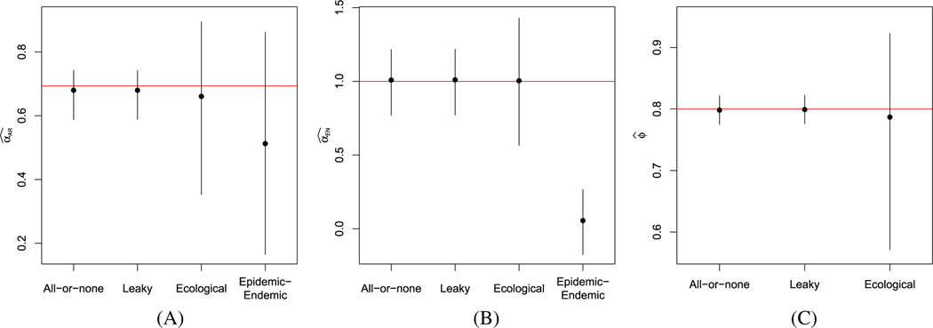
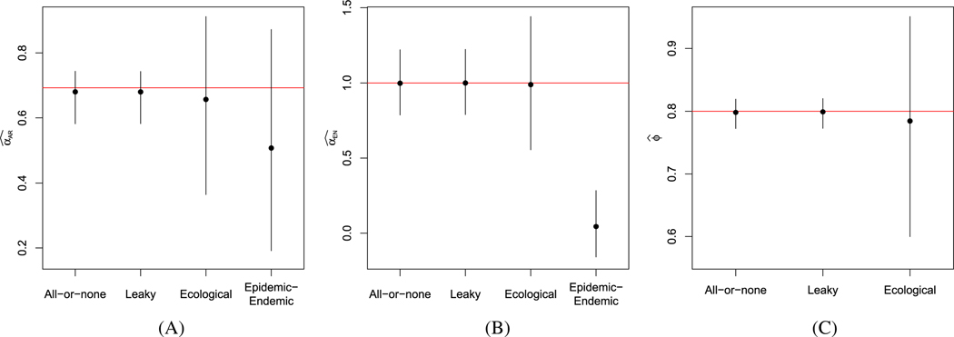
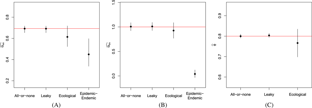
In Figures 3 and 4, we present the average estimates, along with the 2.5- and 97.5-percentiles of estimates obtained under all four models, when the data were simulated assuming an all-or-none or leaky vaccine, respectively. Under all scenarios, the fully observed models yield estimates close to the true model parameters. Compared to the fully observed model estimates, the ecological vaccine model obtains similar estimates, but with wider intervals, appropriately reflecting the lost information as a result of the aggregation. In contrast, the epidemic-endemic models yield estimates that are very different from the true autoregressive and endemic parameter values. We do not include the epidemic-endemic estimates in the pictures for the estimates of the vaccine effect, $\varphi$, since the epidemic-endemic parameter is not comparable to the parameters in the other models.

FIGURE 3.

Summary of simulation results of partially vaccinated populations, assuming an all-or-none vaccine. Average estimates and intervals extending from the 2.5th and 97.5th percentile of estimates across simulations of (A) ${\alpha }_{\text{AR}}$, (B) ${\alpha }_{\text{EN}}$, and (C) $\varphi$ for the fully observed all-or-none and leaky models, the ecological vaccine model, and the epidemic-endemic model. Red horizontal lines denote the true parameter values. A, $\widehat{{\alpha }_{\text{AR}}}\text{;}$ B, $\widehat{{\alpha }_{\text{EN}}}\text{;}$ C, $\widehat{\varphi }$

FIGURE 4.

Summary of simulation results of partially vaccinated populations, assuming an leaky vaccine. Average estimates and intervals extending from the 2.5th and 97.5th percentile of estimates across simulations of (A) ${\alpha }_{\text{AR}}$, (B) ${\alpha }_{\text{EN}}$, and (C) $\varphi$ for the fully observed all-or-none and leaky models, the ecological vaccine model, and the epidemic-endemic model. Red horizontal lines denote the true parameter values. A, $\widehat{{\alpha }_{\text{AR}}}\text{;}$ B, $\widehat{{\alpha }_{\text{EN}}}\text{;}$ C, $\widehat{\varphi }$

These simulations also provide a clear example of the risk for ecological bias when using the epidemic-endemic model. Interpreting the results from the epidemic-endemic model as individual-level parameter estimates would result in erroneous conclusions, especially regarding the endemic risk.

We also consider the results from 20 years’ worth of data in Appendix C and see that, asymptotically, the ecological vaccine model yields unbiased estimates for all model parameters, consistent with the fully observed models.

5 |. APPLICATION TO MEASLES DATA

We now apply the ecological vaccine model to data collected on measles outbreaks in Germany from 2005 through 2007. Measles is a highly contagious viral infection that can result in death for young or malnourished children. The average number of secondary infections that arise from a single measles infection in a completely susceptible population is estimated to be between 15 and 20.^21,22 Fortunately, the measles, mumps, and rubella (MMR) vaccine is very effective. Between 85% and 95% of children will develop immunity after a single dose of the MMR vaccine and a second dose provides nearly 99% vaccine efficacy.²²

Even with an effective vaccine the highly infectious nature of measles means that more than 93% of the population needs to be immune in order to prevent epidemics.^23,24 Hence, even in countries with well establish vaccination programs, such as Germany, small outbreaks persist.

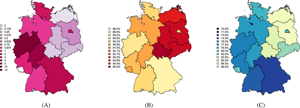
We use data from Germany’s national disease surveillance system, which has been previous used to examine the relationship between vaccination coverage and the size of measles outbreaks and is included in the surveillance package for R.⁹ Further details about this data and previous analysis can be found elsewhere.¹² For our analyses, we assume a two-week time step, based on the approximate generation time for measles.^12,25 Between 2005 and 2007, over 3500 cases of measles were reported throughout Germany, with as many as 344 cases observed in a single biweek. Over the 3 years, no cases were observed in Saarland, and approximately 2000 of those cases were observed in the state of North Rhine-Westphalia (see Figure 5A).

FIGURE 5.

Total number of measles cases per 100 000 observed between 2005 and 2007 (A). Estimated vaccine coverage for at least 1 measles, mumps, and rubella (MMR) vaccination (B) and at least 2 MMR vaccinations (C) in 2006, based on data from examination of vaccination cards in school aged children. A, Cases per 100 000; B, At least 1 MMR vaccination; C, At least 2 MMR vaccinations

Estimated MMR vaccination coverage is based on the number of students presenting vaccination cards at the required medical exam for school entry.¹² Between 87% and 95% of students brought vaccination cards to the entry exam preceding the start of the 2006–2007 school year. Following the previous analysis, we estimate the coverage for at least one MMR vaccine by assuming that the coverage in the population that did not bring the vaccination cards is half that of those who did have vaccination cards.¹² In Figures 5B and 5C, we map the estimated vaccine coverage for one or more MMR vaccines (left) and at least two vaccines (right). Although the available vaccination data is for children starting primary school, typically between 4 and 7 years of age, we assume that the MMR vaccination coverage for the whole population is the same as the estimated vaccination coverage for this analysis. We note that the estimated coverage is likely to be an overestimate, as those who show up for the annual medical exam and bring vaccination cards are more likely to have more complete medical records.¹² We summarize the number of cases and estimated coverage in Table D1.

In this analysis, we are primarily interested in estimating the effects of vaccination on the observed cases of measles. We expand the ecological vaccine model developed in previous sections to incorporate spatial and temporal dependencies. In addition, we adopt a Bayesian paradigm to incorporate our previous knowledge about the MMR vaccine effectiveness.

We fit the following ecological model to the measles data:

$$Y_{i,t+1}\mid {\mu }_{it},\varphi \sim \text{Poisson}\left(N_i\left(1-\varphi x_i\right)\left({\mathit{\lambda }}_i\frac{y_{it}}{N_i}+v_{it}\right)\right),$$ (16)

$$\log {\mathit{\lambda }}_i={\alpha }_{\text{AR}}+a_i,$$

$$\log v_{it}={\alpha }_{\text{EN}}+b_i+\gamma \sin \left({\omega }_t\right)+\delta \cos \left({\omega }_t\right)-\log (N),$$

$$a_i\sim \text{N}\left(0,{\sigma }_{\text{AR}}^2\right),$$

$$b_i\sim \text{N}\left(0,{\sigma }_{\text{EN}}^2\right),$$

$$\varphi \sim \text{Beta}(10,2.5)\text{,}$$

where $x_i$ is the estimated vaccine coverage in area $i$ ; component-specific random effects $a_i$ and $b_i$ are assumed independent;${\omega }_t=2\pi t/26\text{;}$ and the beta prior on $\varphi$ places 90% of the mass is between 0.6 and 0.99. We assume lognormal priors with large variances on ${\alpha }_{\text{AR}}$ and ${\alpha }_{\text{EN}}$. In the formulation of ${\mathit{\lambda }}_i$, we have assumed transmission to be frequency dependent based on previous studies of measles in England and Wales.²⁵ Hamiltonian Monte Carlo sampling via Stan was used to fit this more complex ecological model.²⁶ Corresponding code can be found in the web material.

In Table 2, we summarize the posterior estimates of the fixed effects from the ecological vaccine model. We estimate the vaccine effect to be 0.92, with a 95% posterior credible interval from 0.66 to 0.99, which is commensurate with the known vaccine efficacy for the MMR vaccine. However, this estimate is also similar to the strong prior placed on $\varphi$ (prior 95% interval is from 0.55 to 0.96). Vaccine coverage ranges from 88% to 95% across the 16 German states, and these results suggest that there is little information about the vaccine effect in these data. As a sensitivity analysis, we fit the same hierarchical model with a noninformative prior for $\varphi$. The results are not presented here but can be found in the web material. The noninformative prior on $\varphi$ results in slightly higher estimates for both ${\alpha }_{\text{AR}}$ and $\varphi$, but each has substantially wider credible intervals. The prior choice for $\varphi$ had little effect on the posterior estimates of the parameters in the endemic component of the model.

TABLE 2.

Posterior medians and 95% credible intervals for the parameters of the ecological model for the measles data

	Median	2.5%	97.5%
${\alpha }_{\text{AR}}$	0.91	−0.26	1.66
$\varphi$	0.92	0.66	0.99
${\alpha }_{\text{EN}}$	3.53	2.54	4.16
$\gamma$	0.71	0.55	0.86
$\delta$	−0.20	−0.36	−0.04
${\sigma }_{\text{AR}}$	0.66	0.28	1.61
${\sigma }_{\text{EN}}$	0.52	0.28	0.96
$R_0$	2.49	0.77	5.24

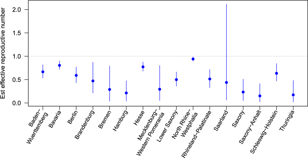
We plot the posterior median and 95% credible intervals for state-specific autoregressive parameters from the ecological vaccine model, computed as $\left(1-\widehat{\varphi }{x}_i\right)\exp \left(\widehat{{\alpha }_{\text{AR}}}+{\widehat{a}}_i\right)$ in Figure 6. Notice that, for the ecological vaccine model, the autoregressive parameter has an intuitive interpretation as the effective reproductive number, where $R=(1-x\varphi )R_0$.¹⁹ As expected, all estimates were below 1, but the area-specific estimates have credible intervals with varying widths. The widest interval was observed for Saarland, and the smallest for North Rhine-Westphalia, the two states with the fewest (0) and most (2036) observed cases over the three-year study.

FIGURE 6.

Estimated state-level autoregressive components. For the ecological vaccine model, posterior median and 95% credible intervals are presented from the Stan model fit

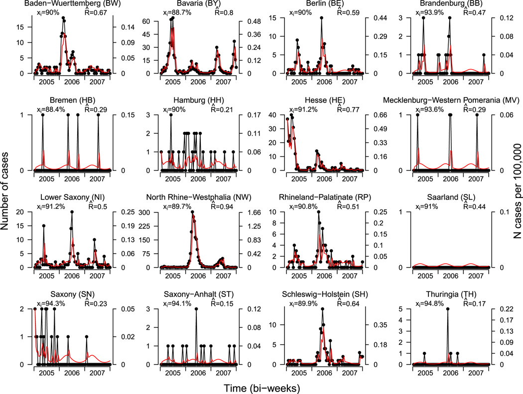
In Figure 7, we plot the total number of observed measles cases and prevalence per 100 000 people, by state and biweek for the 16 states in Germany. The left axis indicates the total number of cases; the right axis indicates the prevalence per 100 000 people. The estimated vaccine coverage and effective reproductive number are included the upper left and right corners of each frame. Fitted values are included in the red and computed following (16) as

$${\widehat{Y}}_{it}=\left(1-\widehat{\varphi }{x}_i\right)\left[\exp \left(\widehat{{\alpha }_{\text{AR}}}+{\widehat{a}}_i\right)Y_{i,t-1}+\left(N_i/N\right)\exp \left(\widehat{{\alpha }_{\text{EN}}}+{\widehat{b}}_i+\widehat{\gamma }\sin \left({\omega }_t\right)+\widehat{\delta }\cos \left({\omega }_t\right)\right)\right]\text{,}$$ (17)

where $Y_{i,t-1}$ is the observed number of counts for area $i$ and week $t-1$, and ${\omega }_t=2\pi t/26$. In general, the ecological vaccine model provides good estimates for the number of cases.

FIGURE 7.

Number of measles cases and prevalence by state and biweek from 2005 through 2007. The left axis indicates the total number of cases; the right axis indicates the prevalence per 100 000 people. Estimated MMR vaccine coverage is included in the upper left corner of each plot. Fitted values from the ecological vaccine model are included in red. Estimated effective reproductive numbers $(\widehat{R})$ is included in the upper right corner

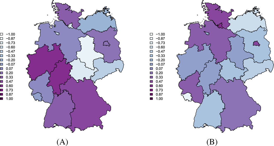
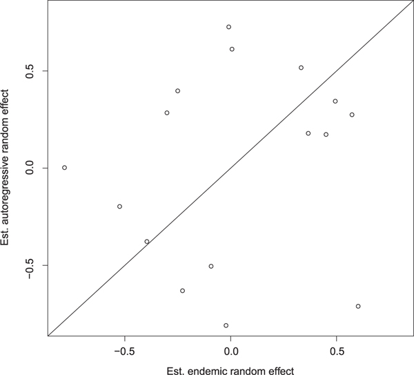
In Figure D1, we plot the area-specific random effects for the autoregressive and endemic components. The states with the highest prevalence have higher autoregressive random effects. The endemic random effects do not appear to have a similar spatial structure as the autoregressive random effects. Moreover, when the autoregressive random effects are plotted against the endemic random effects, as in Figure D2, there is no evidence of a strong correlation between the two components. This supports our decision to model the component-specific random effects as independent. However, in other settings, we may want to consider more complex forms of random effects. For example, if there were strong correlations between the component-specific random effects, it may be more appropriate to assume bivariate normal distribution for the random effects.

In this analysis, the posterior estimate of $R_0$ is 2.49 (95% CI: 0.77 – 5.24), which is much smaller than the typical $R_0$ between 15 and 20 for measles.^21,22 There are many possible sources of this underestimation. Our analyses (and the available data) are in discrete time (biweeks), but in reality, new infections occur in continuous time and space. The discretization of time is known to result in a biased estimate of $R_0$.²⁷ It is likely that large outbreaks, like that in North Rhine-Westphalia in 2006 prompted additional vaccination campaigns. However, we have only a single estimate of vaccination coverage, from children entering school. The estimation of vaccine coverage is likely to not capture the true levels of protection within the population, or the heterogeneity of protection across various age groups.²⁸ Lastly, with any disease surveillance system there is likely to be underreporting of cases. One study of a single German state found that underreporting varied dramatically over the course of the outbreak.²⁹

6 |. DISCUSSION

Infectious disease surveillance data is the primary source of information about disease spread in large populations over time. Current approaches to analyzing these sorts of data tend to focus on prediction, but when used to study covariate effects, the parameter interpretation is cumbersome, especially when the interest is in understanding how vaccination coverage associates with disease. With inference in mind, we started with an individual-level model that included how vaccination affect risk of infection and derived an ecologically consistent model for infectious disease data that accounts for vaccination coverage. A key benefit to our approach is that we obtain estimates of familiar epidemiological parameters, which are easy to interpret (though caveats are in order due to other issues, see the discussion at the end of Section 5). Furthermore, we saw that, under common simplifying assumptions, the resulting ecological vaccine model is the same regardless of the assumed mode of vaccine action. Simulations showed that the ecological vaccine model performs reasonably well in many practical scenarios and illuminated situations when the ecological vaccine model may be inappropriate.

There are limitations to the current model and important extensions to make the approach more broadly applicable. For example, it would be beneficial to extend the ecological vaccine model to account for a nonconstant and perhaps longer infectiousness period. It may be interesting to consider bivariate random effects, or spatially structured random effects in the autoregressive and/or endemic components. Future work will be focused on extending the method to account for stratified population structures and including neighborhood effects in the ecological vaccine model.

Stan and R code to fit the models of this paper can be found in the supporting information for this article at https://github.com/lhfisher/Ecological_Inference.

APPENDIX A. ECOLOGICAL BIAS FOR INFECTIOUS DISEASE MODELS

To better understand ecological bias in the infectious disease setting, we start with a simple individual-level model. Recall, ecological bias occurs when a naïve ecological model is used to make conclusions on individual-level parameters but the implied aggregate risk differs from that of the individual. Let $Y_{itj}$ be the disease indicator for susceptible individual $j$ in week $t$ and area $i$, where $j=1,\dots ,n_i$. Assuming a rare disease so that $1-\exp \left({\mathit{\lambda }}_{itj}^{†}\right)\approx {\mathit{\lambda }}_{itj}^{†}$, we start with the individual-level model

$$Y_{itj}\mid y_{i,t-1}\sim \text{Bernoulli}\left({\mathit{\lambda }}_{itj}^{†}\right),$$ (A1)

where ${\mathit{\lambda }}_{itj}^{†}={\mathit{\lambda }}_{itj}^{\text{AR}}{y}_{i,t-1}/n_i+{\mathit{\lambda }}_{itj}^{\text{EN}}$ and ${\mathit{\lambda }}_{itj}^{\text{AR}}$ and ${\mathit{\lambda }}_{itj}^{\text{EN}}$ are individual-level risks. We additionally assume that the individual risk of infection is a function of some individual-level covariates $z_{itj}$ such that

$${\mathit{\lambda }}_{itj}^{\text{AR}}=e^{{\alpha }_0}f\left({\alpha }_1,z_{itj}\right),$$ (A2)

$${\mathit{\lambda }}_{itj}^{\text{EN}}={\mathit{\lambda }}_{it}^{\text{EN}},$$

where $f\left({\alpha }_1,z\right)$ describes the relationships between the covariate and component-specific risk. In the rare disease setting, the aggregate model for the total number of cases in area $i$ and time $t$ implied by the individual-level model in (A1) and (A2) is

$$Y_{it}\mid y_{i,t-1}\sim \text{Poisson}\left(\overline{{\mathit{\lambda }}_{it}^{\text{AR}}}{y}_{i,t-1}/n_i+\overline{{\mathit{\lambda }}_{it}^{\text{EN}}}\right),$$ (A3)

where $\overline{{\mathit{\lambda }}_{it}^{\text{AR}}}$ and $\overline{{\mathit{\lambda }}_{it}^{\text{EN}}}$ are the aggregate autoregressive and endemic risks. We have assumed a constant endemic risk and, therefore, $\overline{{\mathit{\lambda }}_{it}^{\text{EN}}}=n_i{\mathit{\lambda }}_{it}^{\text{EN}}$. The form of the aggregate autoregressive risk, $\overline{{\mathit{\lambda }}_{it}^{\text{AR}}}$, will depend on the form of the covariate. For a continuous covariate, the autoregressive aggregate risk is

$$\overline{{\mathit{\lambda }}_{it}^{\text{AR}}}=e^{{\alpha }_0}{\int }_{A_i}f\left({\alpha }_1,z\right)g_{it}\left(z\mid {\mathit{\omega }}_{it}\right)dz,$$ (A4)

where $z$ is assumed to be distributed $g_{it}\left(z\mid {\mathit{\omega }}_{it}\right)$, with area- and week-level parameters for that distribution ${\mathit{\omega }}_{it}\text{;}$ and where $A_i$ represents area $i$. For a discrete individual-level covariate, $z_k$ with $K$ levels, the aggregate risk implied by the individual-level model is

$$\overline{{\mathit{\lambda }}_{it}^{\text{AR}}}=e^{{\alpha }_0}\sum _{k=1}^{K}f\left({\alpha }_1,z_k\right)g_{it}\left(z_k\mid {\mathit{\omega }}_{it}\right)\text{.}$$ (A5)

In other words, the consistent aggregated risk is found by averaging the individual-level risk over the distribution of the covariate within area $i$ and week $t$.

However, when only the aggregated data is available, analyses are limited to modeling total number of cases $Y_{it}={\sum }_{j=1}^{n_i}{Y}_{itj}$, and the area- and week-specific average exposures, ${\overline{Z}}_{it}$. It is tempting to fit the naïve ecological regression model

$$\text{E}\left[Y_{it}\mid y_{i,t-1}\right]=\exp \left({\beta }_0+{\beta }_1{\overline{z}}_{it}\right)y_{i,t-1}+\exp \left({\beta }_2\right),$$ (A6)

where $\exp \left({\beta }_1\right)$ is the relative risk of within-area infection associated with a one unit increase in the average exposure, ${\overline{Z}}_{it}$. Therefore, the naïve ecological model assumes the aggregate risk is consistent with the individual-level risk, $\overline{{\mathit{\lambda }}_{it}^{\text{AR}}}=\exp \left({\beta }_0+{\beta }_1{\overline{z}}_{it}\right)$.

Typically, the parameter estimates from (A6) will not be equal to those from implied aggregate model of (A3). The specific form of the implied aggregate risk will, therefore, depend on the within-area distribution of that specific covariate. For example, if $f\left({\alpha }_1,z\right)=\exp \left({\alpha }_{1}z\right)$ and we assume the within-area exposures are distributed normally, ie, $z\mid {\overline{z}}_{it},{\sigma }_{it}^2\sim \text{Normal}\left({\overline{z}}_{it},{\sigma }_{it}^2\right)$, the aggregate risk is

$$\overline{{\mathit{\lambda }}_{it}^{\text{AR}}}=\exp \left({\alpha }_0+{\alpha }_1{\overline{z}}_{it}+{\alpha }_1^2{\sigma }_{it}^2/2\right).$$ (A7)

Thus the consistent aggregate risk is a function of both the average exposure and the variability of that exposure within a given area. Notice that when either the mean and variance are independent or when there is no within-area variability of exposures, ${\sigma }_{it}^2=0$ for all areas $i$ and weeks $t$, the naïve model (A6) is identical to the consistent aggregate model (A7). For further details in a noninfectious disease setting, see the works of Plummer and Clayton³⁰ and Richardson et al.³¹ When the exposure is binary, implied aggregate risk is

$$\overline{{\mathit{\lambda }}_{it}^{\text{AR}}}=e^{{\alpha }_0}\left[\left(1-{\overline{z}}_{it}\right)+{\overline{z}}_{it}{e}^{{\alpha }_1}\right],$$ (A8)

where ${\overline{z}}_{it}$ is the proportion of exposed individuals in area $i$ and week $t$.

In the noninfectious disease setting, it is well understood that, when data are aggregated to the group level, individual-level associations can become distorted, leading to ecological bias. In some ways, it is misleading to refer to this difference as bias. Both the implied aggregate and naïve model will produce unbiased estimates of different parameters. The naïve model estimates the risk associated with the average exposure, whereas the implied aggregate model estimates the average of individual risks.³² The ‘bias’ comes from trying to estimate individual-level associations from a model that estimates average parameters.

APPENDIX B. ECOLOGICAL VACCINE MODEL IDENTIFIABILITY

We derive the ecological vaccine model when the vaccine’s mode of action is a combination of both leaky and all-or-none. Following the development in Section 3, we assume that a vaccine fails with probability $\theta$ and, when it takes, reduces risk of infection by $\varphi$. Individuals will fit into one of three groups: unvaccinated, failed vaccinated, and vaccinated subscripted by $u$, $f$, and $v$, respectively. Let $x$ be the proportion of vaccinated individuals in a fully susceptible population of size $N$. Hence, the initial susceptible population will be

$$S_{u0}=(1-x)N,S_{f0}=(1-\theta )xN,S_{v0}=\theta xN.$$

The force of infection for each group is defined as

$${\mathit{\lambda }}_{ut}^{†}={\mathit{\lambda }}_t^{†},{\mathit{\lambda }}_{ft}^{†}={\mathit{\lambda }}_t^{†},{\mathit{\lambda }}_{vt}^{†}=(1-\varphi ){\mathit{\lambda }}_t^{†}\text{.}$$

Together, these define disease progression

$$Y_{u,t+1}\mid {\mathit{\lambda }}_{ut}^{†}\sim \text{Binomial}\left(S_{ut},1-e^{-{\mathit{\lambda }}_t^{†}}\right),$$

$$Y_{f,t+1}\mid {\mathit{\lambda }}_{ut}^{†}\sim \text{Binomial}\left(S_{ft},1-e^{-{\mathit{\lambda }}_t^{†}}\right),$$

$$Y_{v,t+1}\mid {\mathit{\lambda }}_{ut}^{†}\sim \text{Binomial}\left(S_{vt},1-e^{-(1-\varphi ){\mathit{\lambda }}_t^{†}}\right),$$

where $S_{gt}=S_{g0}-{\sum }_{s=1}^t{Y}_{gs}$, for $g=\{u,f,v\}$. Furthermore, the aggregated model is a convolution of the binomials (and unvaccinated and failed vaccinated groups can be combined into a single group). When the binomial distributions can be approximated by Poisson distributions, this implies

$$Y_{t+1}\mid {\mathit{\lambda }}_t^{†}\sim \text{Poisson}\left(\left(S_{ut}+S_{ft}\right)\left(1-e^{-{\mathit{\lambda }}_t^{†}}\right)+S_{vt}1-e^{-(1-\varphi ){\mathit{\lambda }}_t^{†}}\right).$$

The Taylor approximation simplifies the above, ie,

$$Y_{t+1}\mid {\mathit{\lambda }}_t^{†}\sim \text{Poisson}\left(\left(S_{ut}+S_{ft}+(1-\varphi )S_{vt}\right){\mathit{\lambda }}_t^{†}\right).$$

Moreover, when the number of infections is negligible, so that the number of susceptibles is approximately the initially susceptible population, we arrive at the ecological vaccine model

$$Y_{t+1}\mid {\mathit{\lambda }}_t^{†}\sim \text{Poisson}\left((1-\varphi \theta x)N{\mathit{\lambda }}_t^{†}\right).$$ (B1)

Notice that, in the above, the specific modes of vaccine action (all-or-none or leaky) cannot be identified with aggregate data.

APPENDIX C. ASYMPTOTIC BEHAVIOR OF THE ECOLOGICAL VACCINE MODEL

Under the same conditions as the simulations in Section 4.2, we considered the results for 10 years’ worth of data. In Figure C1, we present estimates from the fully observed all-or-none and leaky models, along with estimates from the ecological vaccine model and the epidemic-endemic model. We see that the estimates for the fully observed models, as well as the ecological vaccine models are much closer to the true parameter values compared to the previous simulations, which used only 3 years of weekly data. With long time series, the ecological vaccine model provides unbiased estimates for all model parameters.

APPENDIX D. ADDITIONAL RESULTS FROM MEASLES ANALYSIS

Table D1 presents the total number of measles cases and the estimates of vaccination coverage for the 16 states of Germany.

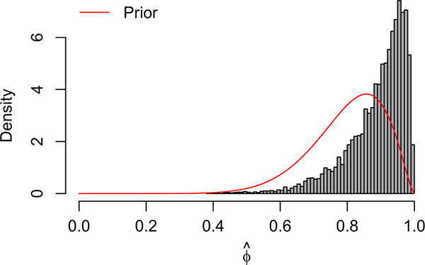
In Figure D3, we plot a histogram of posterior samples of $\widehat{\varphi }$ along with the prior Beta(10, 2.5) curve. The posterior is similar to the prior, suggesting that there is little information about the vaccine effect in this data. As a sensitivity analysis, we fit the same hierarchical model with a noninformative prior for $\varphi$. The noninformative prior on $\varphi$ results in slightly higher estimates for both ${\alpha }_{\text{AR}}$ and $\varphi$, but each has substantially wider credible intervals. The prior choice for $\varphi$ had little effect on the posterior estimates of the parameters in the endemic component of the model.

FIGURE D1.

Maps of the random effect estimates for the autoregressive and endemic components in the ecological vaccine model A, AR random effects; B, EN random effects

FIGURE D2.

Comparison of autoregressive and endemic random effect estimates

FIGURE D3.

Histogram of posterior samples of $\widehat{\varphi }$. The red curve is the prior distribution, Beta(10, 2.5)

FIGURE C1.

Estimates and 95% confidence intervals for the fully observed all-or-none and leaky models, the ecological vaccine model, and the epidemic-endemic model for 10 years’ worth of weekly data simulated assuming an all-or-none vaccine. Red horizontal lines denote the true parameter values. A, $\widehat{{\alpha }_{\text{AR}}}\text{;}$ B, $\widehat{{\alpha }_{\text{EN}}}\text{;}$ C, $\widehat{\varphi }$

TABLE D1.

Number of measles cases and estimated vaccination coverage for the 16 German states from 2005–2007. Estimated vaccination coverage for at least 1 or 2 MMR vaccinations and comes from the school entry examinations. Note this partially reproduces Table 1 from previous analyses¹²

			Est. Coverage (%)
State (Abbreviation)	Population	Total Cases	1st dose	2nd dose
Baden-Wuerttemberg (BW)	10,738,753	162	90.0%	75.6%
Bavaria (BY)	12,492,658	606	88.7%	73.2%
Berlin (BE)	3,404,037	104	90.0%	80.2%
Brandenburg (BB)	2,547,772	18	93.9%	86.9%
Bremen (HB)	663,979	4	88.4%	71.9%
Hamburg (HH)	1,754,182	29	90.0%	80.5%
Hesse (HE)	6,075,359	336	91.2%	78.1%
Mecklenburg-Western Pomerania (MV)	1,693,754	4	93.6%	88.0%
Lower Saxony (NI)	7,982,685	144	91.2%	78.0%
North Rhine-Westphalia (NW)	18,028,745	2,036	89.7%	76.9%
Rhineland-Palatinate (RP)	4,052,860	85	90.8%	77.3%
Saarland (SL)	1,043,167	0	91.0%	81.8%
Saxony (SN)	4,249,774	18	94.3%	82.4%
Saxony-Anhalt (ST)	2,441,787	12	94.1%	86.5%
Schleswig-Holstein (SH)	2,834,254	89	89.9%	79.3%
Thuringia (TH)	2,311,140	8	94.8%	85.9%

DATA AVAILABILITY STATEMENT

The data and code for both the simulations and data analysis presented in this manuscript are available at https://github.com/lhfisher/Ecological_Inference.

REFERENCES

- 1.Selvin HC. Durkheim’s ‘suicide’ and problems of empirical research. Am J Sociol. 1958;63:607–619. [Google Scholar]
- 2.Robinson WS. Ecological correlations and the behavior of individuals. Am Sociol Rev. 1950;15:351–357. [Google Scholar]
- 3.Greenland S. Divergent biases in ecologic and individual level studies. Statist Med. 1992;11:1209–1223. [DOI] [PubMed] [Google Scholar]
- 4.Greenland S, Robins J. Ecological studies: biases, misconceptions and counterexamples. Am J Epidemiol. 1994;139:747–760. [DOI] [PubMed] [Google Scholar]
- 5.Richardson S, Monfort C. Ecological correlation studies. In: Elliott P, Wakefield JC, Best NG, Briggs DJ, eds. Spatial Epidemiology: Methods and Application. Oxford, UK: Oxford University Press; 2000. [Google Scholar]
- 6.Wakefield J. Ecologic studies revisited. Annu Rev Public Health. 2008;29:75–90. [DOI] [PubMed] [Google Scholar]
- 7.Wakefield J, Lyons H. Spatial aggregation and the ecological fallacy. In: Gelfand A, Diggle P, Guttorp P, Fuentes M, eds. Handbook of Spatial Statistics. Boca Raton, FL: CRC Press; 2010. [Google Scholar]
- 8.Finkenstädt BF, Grenfell BT. Time series modelling of childhood diseases: a dynamical systems approach. J Royal Stat Soc Ser C (Appl Stat). 2000;49(2):187–205. [Google Scholar]
- 9.Held L, Höhle M, Hofmann M. A statistical framework for the analysis of multivariate infectious disease surveillance counts. Stat Model. 2005;5:187–199. [Google Scholar]
- 10.Paul M, Held L, Toschke AM. Multivariate modelling of infectious disease surveillance data. Stat Med. 2008;27:6250–6267. [DOI] [PubMed] [Google Scholar]
- 11.Paul M, Held L. Predictive assessment of a non-linear random effects model for multivariate time series of infectious disease counts. Statist Med. 2011;30:1118–1136. [DOI] [PubMed] [Google Scholar]
- 12.Herzog SA, Paul M, Held L. Heterogeneity in vaccination coverage explains the size and occurrence of measles epidemics in German surveillance data. Epidemiol Infect. 2011;139:505–515. [DOI] [PubMed] [Google Scholar]
- 13.Meyer S, Held L. Power-law models for infectious disease spread. Ann Appl Stat. 2014;8:1612–1639. [Google Scholar]
- 14.Meyer S, Held L, Höhle M. Spatio-temporal analysis of epidemic phenomena using the R package surveillance. J Stat Softw. 2017;77(11). [Google Scholar]
- 15.Bauer C, Wakefield J. Stratified space-time infectious disease modeling: with an application to hand, foot and mouth disease in China. J Royal Stat Soc Ser A. 2018;67:1379–1398. [Google Scholar]
- 16.Xia Y, Bjørnstad ON, Grenfell BT. Measles metapopulation dynamics: a gravity model for epidemiological coupling and dynamics. Am Nat. 2004;164:267–281. [DOI] [PubMed] [Google Scholar]
- 17.Wakefield J, Dong T, Minin V. Spatio-temporal analysis of surveillance data. In: Gelfand A, Diggle P, Guttorp P, Fuentes M, eds. Handbook of Spatial Statistics: Boca Raton, FL: CRC Press; 2019. [Google Scholar]
- 18.Koopman JS, Longini IM. The ecological effects of individual exposures and nonlinear disease dynamics in populations. Am J Public Health. 1994;84:836–842. [DOI] [PMC free article] [PubMed] [Google Scholar]
- 19.Halloran ME, Longini IM, Struchiner CJ. Design and Analysis of Vaccine Studies. New York, NY: Springer; 2010. [Google Scholar]
- 20.Van Boeckel TP, Takahashi S, Liao Q, et al. Hand, foot, and mouth disease in China: critical community size and spatial vaccination strategies. Scientific Reports. 2016;6(1):25248. [DOI] [PMC free article] [PubMed] [Google Scholar]
- 21.Keeling MJ, Rohani P. Modeling Infectious Diseases in Humans and Animals. Princeton, NJ: Princeton University Press; 2008. [Google Scholar]
- 22.Sudfeld CR, Navar AM, Halsey NA. Effectiveness of measles vaccination and vitamin A treatment. Int J Epidemiol. 2010;39:i48–i55. [DOI] [PMC free article] [PubMed] [Google Scholar]
- 23.Centers for Disease Control and Prevention. Measles, mumps, and rubella – vaccine use and strategies for elimination of measles, rubella, and congenital rubella syndrome and control of mumps: recommendations of the advisory committee on immunization practices (ACIP). MMWR. 1998;47(RR-8):1–58. [PubMed] [Google Scholar]
- 24.World Health Organization. Measles vaccines: WHO position paper. Wkly Epidemiol Rec. 2009;84:349–360. [PubMed] [Google Scholar]
- 25.Bjørnstad ON, Finkenstädt BF, Grenfell BT. Dynamics of measles epidemics: estimating scaling of transmission rates using a time series SIR model. Ecol Monogr. 2002;72:169–184. [Google Scholar]
- 26.Carpenter B, Gelman A, Hoffman MD, et al. Stan: a probabilistic programming language. J Stat Softw. 2017;76(1). [DOI] [PMC free article] [PubMed] [Google Scholar]
- 27.Ferrari MJ, Bjørnstad ON, Dobson AP. Estimation and inference of of an infectious pathogen by a removal method. Math Biosci. 2005;198(1):14–26. [DOI] [PubMed] [Google Scholar]
- 28.Poethko-Müller C, Mankertz A. Seroprevalence of measles-, mumps- and rubella-specific IgG antibodies in German children and adolescents and predictors for seronegativity. PLOS ONE. 2012;7(8):1–13. [DOI] [PMC free article] [PubMed] [Google Scholar]
- 29.Mette A, Reuss AM, Feig M, et al. Under-reporting of measles–an evaluation based on data from North Rhine-Westphalia. Dtsch Arztebl Int. 2011;108(12):191–196. [DOI] [PMC free article] [PubMed] [Google Scholar]
- 30.Richardson S, Stucker I, Hémon D. Comparison of relative risks obtained in ecological and individual studies: some methodological considerations. Int J Epidemiol. 1987;16:111–120. [DOI] [PubMed] [Google Scholar]
- 31.Plummer M, Clayton D. Estimation of population exposure. J Royal Stat Soc Ser B. 1996;58:113–126. [Google Scholar]
- 32.Wakefield J, Haneuse S, Dobra A, Teeple E. Bayes computation for ecological inference. Statist Med. 2011;30:1381–1396. [DOI] [PMC free article] [PubMed] [Google Scholar]
Associated Data
This section collects any data citations, data availability statements, or supplementary materials included in this article.