A Low-Rank Deep Image Prior Reconstruction for Free-Breathing Ungated Spiral Functional CMR at 0.55T and 1.5T

Abstract

Object:

This study combines a deep image prior with low-rank subspace modeling to enable real-time (free-breathing and ungated) functional cardiac imaging on a commercial 0.55T scanner.

Materials and Methods:

The proposed low-rank deep image prior (LR-DIP) uses two u-nets to generate spatial and temporal basis functions that are combined to yield dynamic images, with no need for additional training data. Simulations and scans in 13 healthy subjects were performed at 0.55T and 1.5T using a golden angle spiral bSSFP sequence with images reconstructed using l₁-ESPIRiT, low-rank plus sparse (L+S) matrix completion, and LR-DIP. Cartesian breathheld ECG-gated cine images were acquired for reference at 1.5T. Two cardiothoracic radiologists rated images on a 1-5 scale for various categories, and LV function measurements were compared.

Results:

LR-DIP yielded the lowest errors in simulations, especially at high acceleration factors (R≥8). LR-DIP ejection fraction measurements agreed with 1.5T reference values (mean bias −0.3% at 0.55T and −0.2% at 1.5T). Compared to reference images, LR-DIP images received similar ratings at 1.5T (all categories above 3.9) and slightly lower at 0.55T (above 3.4).

Conclusion:

Feasibility of real-time functional cardiac imaging using a low-rank deep image prior reconstruction was demonstrated in healthy subjects on a commercial 0.55T scanner.

Introduction

Cardiac magnetic resonance (CMR) imaging is the gold standard modality for evaluating left ventricular (LV) function, and cine balanced steady-state free precession (bSSFP) sequences are a cornerstone of most CMR protocols [1]. Conventional cine scans employ a segmented Cartesian readout with electrocardiogram (ECG) gating to minimize motion artifacts, with 1-2 slices acquired during a breathhold. One limitation is that failed breathholds and ECG mis-gating may lead to motion artifacts and require repeated scans. Thus, real-time (i.e., free-breathing and ungated) techniques are often used in patients who cannot perform breathholds or have irregular cardiac rhythms. Various rapid imaging strategies have been developed for real-time functional CMR, including parallel imaging [2–7], k-t methods [8, 9], compressed sensing [10–13], and low-rank subspace reconstructions [14–18].

While most clinical CMR exams are performed at 1.5T and 3T, there has been renewed interest in scanners that operate at lower magnetic field strengths, such as 0.55T [19, 20]. The potential advantages of low-field CMR include lower scanner costs, decreased susceptibility effects and bSSFP banding artifacts, and lower specific absorption rates [21], which allow the use of high flip angles to improve blood-myocardium contrast with bSSFP sequences [22, 23] and may improve safety for patients with implanted metallic devices [24]. However, low-field CMR faces several challenges. One limitation is the reduced signal-to-noise ratio (SNR) that scales approximately linearly with field strength, although the decrease in T₁ and increase in T₂* can be leveraged to offset this effect partially [19]. Low-field scanners tend to have fewer receiver coils with suboptimal geometry that may limit parallel imaging performance. Although not an inherent limitation of low-field imaging, lower-cost commercial 0.55T systems currently lack ECG gating capability. Thus, while several studies have employed ECG-gated cine imaging on clinical 1.5T scanners ramped down to operate at 0.55T [19, 22, 25], studies on commercial 0.55T systems with lower gradient performance and no ECG-gating capability have focused on real-time imaging [26–28].

Deep learning reconstructions have shown great promise for mitigating noise and undersampling artifacts for breathheld and ECG-gated cine acquisitions at 1.5T and 3T [29–31]. These methods typically employ supervised training of a neural network on large numbers of ground truth datasets. However, supervised training for real-time CMR is challenging because respiratory and cardiac motion typically prevent the collection of fully sampled images. To circumvent this issue, synthetic training data can be generated by retrospectively undersampling gated cine acquisitions [32–34], or real-time images can be reconstructed using compressed sensing (or other methods) to serve as training examples [35]. However, these solutions may not necessarily translate well to low-field MRI. The low SNR can make it difficult to obtain high-quality (low noise) real-time images for network training, and it is not possible to acquire gated cine images that can be retrospectively undersampled on commercial 0.55T systems that lack gating capability. For these reasons, self-supervised deep learning reconstructions that are trained using undersampled k-space data are an attractive option for real-time CMR, especially at 0.55T.

This study expands upon the deep image prior (DIP) technique introduced by Ulyanov et al. In the original DIP technique, a convolutional network learned to generate a denoised image using only the noise-corrupted image as training data [36]. The network structure (based on a u-net) was designed to recover lower spatial frequencies at a faster rate during training than higher spatial frequencies [37], so that high-frequency noise could be rejected by employing early stopping or dropout regularization [38]. In the context of MRI, DIP techniques have been applied to diffusion-weighted imaging [39], multi-echo GRE [40], cardiac MR Fingerprinting T₁ and T₂ mapping [41], and real-time functional CMR at 1.5T [42].

This study proposes a self-supervised deep learning reconstruction for dynamic imaging, applied to real-time CMR at both 1.5T and 0.55T. This technique will be referred to as a low-rank deep image prior (LR-DIP), as it combines the DIP framework with low-rank subspace approaches [14] to compactly represent a time series of images using a small number of basis functions. Two u-nets separately generate spatial and temporal basis functions, which are combined to yield dynamic images. Training is performed de novo after each scan by enforcing consistency between the generated images and the acquired k-space data. In this work, LR-DIP is applied to free-breathing ungated bSSFP CMR imaging with spiral golden angle sampling both at 1.5T and on a commercial 0.55T scanner with lower performance gradients and no ECG gating capability, with validation in simulations and healthy subjects. Image quality ratings and LV functional measurements are compared to (1) real-time images at 0.55T and 1.5T, reconstructed using parallel imaging and compressed sensing (l₁-ESPIRiT) and a low-rank plus sparse (L+S) technique, and (2) conventional breathheld ECG-gated cine images acquired at 1.5T.

Materials and Methods

GROG Preprocessing

Spiral k-space data were preprocessed using GRAPPA Operator Gridding (GROG) to avoid time-consuming non-uniform fast Fourier Transform (NUFFT) operations [43] during the LR-DIP reconstruction, which requires repeated iterations between k-space and image domains. GROG is a parallel imaging method for shifting non-Cartesian k-space data to their nearest Cartesian grid points [44]. The first step is to calculate the unit shift operators, which are coil weighting factors needed to shift k-space data by a unit distance along each axis (Δk_x = 1 and Δk_y = 1). This calibration step is typically performed using fully sampled data. Here, the dynamic spiral k-space data were averaged over time and interpolated onto Cartesian k-space coordinates using convolution gridding; this data was used to calibrate the unit shift operators. Next, the weighting factors needed to shift k-space data by a smaller distance (Δk < 1) in any direction can be derived from the unit shift operators. In this way, GROG was applied to each temporal frame of the spiral scan to yield undersampled Cartesian k-space data, which will be denoted y_i for the i^th frame. P_i will denote a sampling mask; if a spiral data point was shifted to a particular Cartesian grid location, the mask at that location contained a 1 instead of a 0. The density compensation function W was calculated by counting the number of spiral k-space points that were shifted to each Cartesian coordinate, as described in [44].

Neural Network Architecture

The LR-DIP reconstruction used two u-nets to generate spatial $\left(u_k\in {\mathbb{C}}^{n_y\times n_x\times k}\right)$ and temporal $\left(v_k\in {\mathbb{C}}^{k\times t}\right)$ basis functions, where n_y and n_x denote the image matrix size, t is the number of time frames, and k is the subspace rank. Both networks were randomly initialized without prior training. As shown in Figure 1, a u-net (denoted by θ_S) with 2D convolutional layers and five downsampling/upsampling paths was used to generate the spatial basis functions. Each convolution was followed by leaky ReLU activation, batch normalization, and dropout. Downsampling was implemented using strided convolution, and upsampling was performed using nearest neighbor interpolation. The input to the network was a tensor $z_S\in {\mathbb{R}}^{n_y\times n_x\times d}$ initialized with uniform random numbers between −0.1 to 0.1 as in the original DIP publication [36], with d denoting the number of feature maps in the input tensor (fixed at d=32 for this study). The network output had size n_y × n_x × (2k) and contained the interleaved real and imaginary parts of the k spatial basis functions. A similar u-net was used to generate the temporal basis functions, although this network performed 1D rather than 2D convolutions. The input to the network, $z_T\in {\mathbb{R}}^{t\times d}$, was initialized with uniform random numbers. The output had size t × (2k) and contained the interleaved real and imaginary parts of the temporal basis functions.

Figure 1.

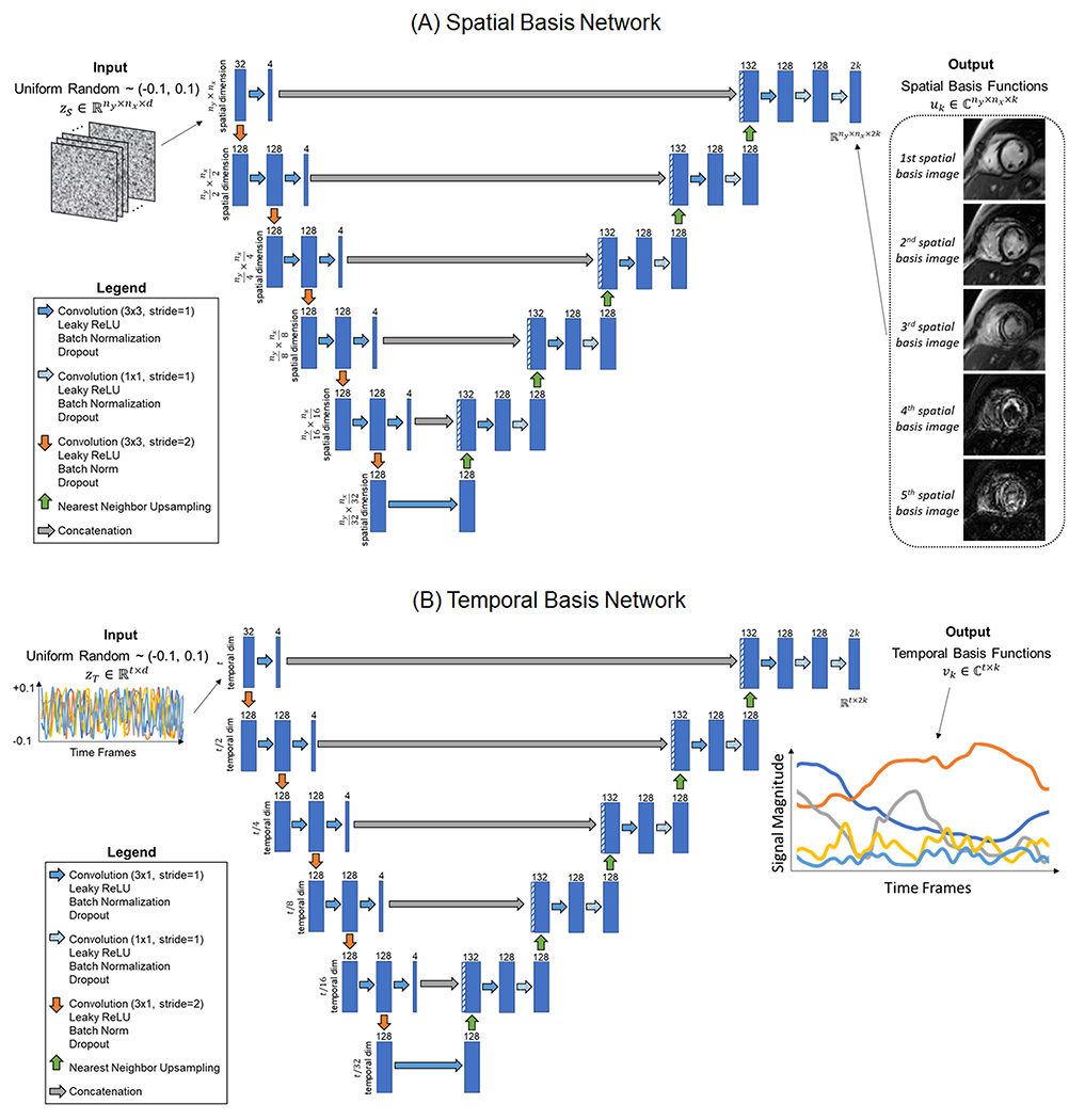
U-net architectures used to generate the (A) spatial and (B) temporal basis functions. Both networks consisted of convolutional layers with five downsampling and upsampling paths. Two-dimensional (2D) convolutions were used in the spatial network, while one-dimensional (1D) were used in the temporal network. The input to each network was a tensor of random uniform numbers, which remained fixed during training.

Self-Supervised Training

After each acquisition, the spatial and temporal basis networks were trained de novo by enforcing consistency between the generated images and the undersampled k-space measurements (Figure 2). First, the input tensors (z_S and z_T) and network weights (θ_S and θ_T) were randomly initialized. The inputs remained fixed during training, and only the network weights were updated. On each iteration, the basis functions generated by the networks were multiplied to yield a time series of images, denoted by x

$$u_k={\theta }_S\left(z_S\right)$$ [1]

$$v_k={\theta }_T\left(z_T\right)$$ [2]

$$x=u_k{v}_k^{\mathrm{*}}$$ [3]

A subset of b image frames was selected for every iteration as a mini-batch to limit memory usage. In practice, mini-batch selection was implemented by replacing $v_k^{*}$ in Equation 3 by $v_{k,b}^{*}$ (which contains only the columns from $v_k^{*}$ corresponding to the b time frames in the mini-batch), so that multiplying u_k by $v_{k,b}^{*}$ yielded only the frames in the mini-batch rather than the entire time series. The images in each mini-batch were multiplied by coil sensitivity maps (denoted by S), transformed to Cartesian k-space using a 2D FFT, and multiplied by the k-space sampling mask (denoted by P_i for the i^th frame). The resulting multichannel k-space data in a given frame i, denoted by ${\tilde{y}}_i$ are given by the following expression

$${\tilde{y}}_i=P_{i}FS{x}_i$$ [4]

The mean squared error (MSE) loss was calculated between the estimated (${\tilde{y}}_i$) and acquired (y_i) k-space data after density compensation, and the network weights were updated using backpropagation.

$$\underset{{\mathit{\theta }}_{\mathit{s}},{\mathit{\theta }}_{\mathit{t}}}{\min }\sum {‖W\left({\tilde{y}}_i-y_i\right)‖}_2^2$$ [6]

Figure 2.

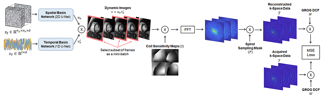
Self-supervised training of the low-rank deep image prior. Training was performed de novo after each new acquisition, with no prior knowledge of the temporal dynamics and no additional training data. On each iteration, the two u-nets generated spatial and temporal basis functions u_k and v_k, which were multiplied to yield dynamic images $x=u_k{v}_k^{*}$ (with * denoting the conjugate transpose). A different subset of image frames was selected as a minibatch during each iteration. The image frames in the minibatch were multiplied by coil sensitivity maps, transformed to k-space using an FFT operation, and multiplied by the golden angle spiral k-space sampling mask. The resulting k-space data, $\tilde{y}$, were compared to the acquired k-space data, $\tilde{y}$, after density compensation using a mean squared error (MSE) loss function, and the spatial and temporal basis networks were updated using backpropagation. The spiral k-space data were preprocessed using GROG to allow use of FFT operations rather than non-uniform fast Fourier Transform (NUFFT) operations, which are more time-consuming.

Training was performed for 20,000 iterations using an Adam optimizer with a learning rate of 0.001 and a batch size of 8 frames. During the final 1000 iterations, the basis functions generated by the network were averaged using an exponential sliding window with a weight of 0.99 to smooth out instabilities during training due to stochastic gradient descent, as described in [36], and the basis functions were combined using Equation 3 to yield the dynamic images. The reconstruction was implemented on a high-performance cluster with one GPU node running Tensorflow 2.8 with a Keras backend. The reconstruction code is publicly available at https://github.com/hamiljes/LowRankDeepImagePrior_RealTimeCine.

Simulations

The LR-DIP reconstruction was first evaluated in simulations using the XCAT phantom [45]. T₁, T₂, and proton density maps were generated using literature values for 0.55T, including T₁=700ms and T₂=60ms for myocardium [19]. A bSSFP sequence was simulated from the maps using a flip angle of 105°, TR/TE 6.30/3.15ms, and a matrix size of 128x128 to match the in vivo imaging parameters. Images were multiplied by simulated 8-coil sensitivity maps and sampled with a golden angle spiral trajectory using the NUFFT. Realistic respiratory (3.9 breaths per minute) and cardiac motion (75 beats per minute) were simulated as follows. Taking an acceleration factor of R=8 (6 spiral interleaves per frame) as an example, each interleaf was sampled using a different image having a small amount of motion in between (one image per TR), and the average of the 6 images was taken as the ground truth. Data were simulated for 768 TRs, corresponding to an acquisition time of 4.8 seconds. Accuracy was quantified by calculating the root mean square error (RMSE), structural similarity index measure (SSIM), and peak signal-to-noise ratio (pSNR) for each frame and reporting the average over all frames.

First, the effect of varying the subspace rank was evaluated. Data were simulated with an acceleration factor of R=8 (6 interleaves per frame, 38 ms temporal resolution, 128 frames), and the LR-DIP reconstruction was performed with ranks ranging from 3 to 128. Second, the reconstruction was repeated with dropout levels ranging from 0% to 50% during training, as dropout was expected to prevent overfitting to noise and aliasing artifacts. These simulations used a fixed acceleration factor of R=8 and a subspace rank of 40. Third, the LR-DIP technique was compared to compressed sensing and low-rank subspace reconstructions at different acceleration factors. The same dataset was used for these simulations, as different acceleration factors could be obtained by binning a different number of spiral interleaves per frame due to the golden angle ordering [46]. The following acceleration factors were tested: R=6 (8 interleaves/frame, 50 ms temporal resolution, 96 total frames), R=8 (6 interleaves/frame, 38 ms temporal resolution, 128 total frames), and R=12 (4 interleaves/frame, 25 ms temporal resolution, 192 total frames). Images were reconstructed using LR-DIP with 10% dropout and rank 40. For comparison, images were also reconstructed using l₁-ESPIRiT with spatial and temporal total variation penalties of 0.003 and 0.02 relative to the maximum image intensity and 25 iterations of conjugate gradient descent [7], and low-rank plus sparse (L+S) matrix decomposition with 50 iterations and penalties of 0.02 and 0.1 for the low-rank (λ_L) and sparse (λ_S) terms [17].

Validation in Healthy Subjects

Data Acquisition

Data were collected in 11 healthy subjects who were scanned in back-to-back sessions on 0.55T (Free.Max, MAGNETOM Siemens, Erlangen, Germany) and 1.5T (Sola, MAGNETOM Siemens) scanners after obtaining written informed consent in this HIPAA-compliant, IRB-approved study. A short-axis stack of free-breathing ungated 2D bSSFP scans with full LV coverage was acquired at both field strengths. Additional scan parameters are given in Table 1. A higher flip angle of 105° was used at 0.55T to improve the contrast between myocardium and blood [24] compared to 55-70° at 1.5T, which was possible due to the decreased SAR at 0.55T. Different spiral trajectories were employed for each field strength, with the 0.55T spiral designed to satisfy the lower gradient amplitude and slew rate limits of the low-field system. Both spirals required 24 interleaves to sample the central 25% of k-space and 48 interleaves to fully sample the periphery of k-space, with the spiral rotated by the golden angle every TR [46]. The total scan time was 4.8 seconds per slice. Due to the longer TR employed at 0.55T than 1.5T (6.3 ms versus 5.1 ms), fewer total interleaves were collected at 0.55T (768 versus 940 total interleaves).

Table 1.

Acquisition parameters for free-breathing ungated spiral bSSFP cardiac scans

Acquisition Parameters	1.5T	0.55T
Readout Duration (ms)	3.4	3.8
Max Gradient Amplitude (mT/m)	26	13
Max Gradient Slew Rate (mT/m/ms)	130	34
Matrix Size	192	128
FOV (mm2)	295 x 295	280 x 280
In-Plane Resolution (mm2)	1.5 x 1.5	2.2 x 2.2
Slice Thickness (mm)	8	8
Number of Slices	10-12	10-12
Slice Gap	20-25%	20-25%
TR	5.1	6.3
TE	1.4	1.8
Flip Angle (°)	55-75°	105°
Number of Receiver Coils	28-34	12-15
Acquisition Time Per Slice (s)	4.8	4.8
Total Number of Interleaves (TRs)	940	768

A Cartesian cine scan was acquired at 1.5T to provide reference measurements of LV volumes and function. This scan was ECG-gated with 25 cardiac phases, and one slice was imaged in a breathhold of 6.2 seconds. Other imaging parameters included TR 4.0 ms, TE 2.0 ms, GRAPPA R=2, 340x336 mm² FOV, and 1.5x1.5x8.0 mm³ resolution.

Image Reconstruction

The real-time data were reconstructed at a temporal resolution of 38 ms at 0.55T (R=8, 6 interleaves/frame, 128 total frames) and 41 ms at 1.5T (R=6, 8 interleaves/frame, 117 total frames). All data were reconstructed using l₁-ESPIRiT, L+S matrix completion, and LR-DIP with a subspace rank of 40 and dropout levels of 10% for 0.55T datasets and 5% for 1.5T datasets. In three subjects, the LR-DIP reconstruction was repeated using dropout levels ranging from 0% to 30% to investigate the impact of dropout on image quality at both field strengths. Since the temporal resolution can be adjusted retrospectively due to the golden angle ordering, one 0.55T dataset was reconstructed and compared using l₁-ESPIRiT, L+S, and LR-DIP with acceleration factors of R=4 (76 ms/frame, 64 frames), R=6 (50 ms/frame, 96 frames), R=8 (38 ms/frame, 128 frames), R=12 (25 ms/frame, 192 frames), and R=24 (13 ms/frame, 384 frames).

Image and Statistical Analysis

The contrast-to-noise ratio (CNR) between myocardium and blood was measured using the following equation, where μ_myo and μ_blood were the mean pixel intensities in regions of interest (ROIs) containing predominantly myocardium or blood, and σ_noise was the standard deviation within an ROI placed in the background

$$CNR=\frac{\left|{\mu }_{myo}-{\mu }_{blood}\right|}{{\sigma }_{noise}}$$ [7]

A single CNR value per subject was obtained by averaging the CNR from two images at peak diastole and peak systole. The mean and standard deviation of the CNR were computed over all subjects, and differences among methods were compared using a within-subjects ANOVA test.

One cardiothoracic radiologist manually segmented the endocardial borders on the reference 1.5T Cartesian cine, real-time 1.5T LR-DIP, and real-time 0.55T LR-DIP datasets using ITK-SNAP [47]. End-diastolic (EDV), end-systolic volume (ESV), and left ventricular ejection fraction (LVEF) were calculated using Simpson’s method. Because the real-time images spanned multiple heartbeats, one frame at peak diastole and one at peak systole were selected before segmenting the images. ESV, EDV, and LVEF from real-time scans were compared to reference measurements using a Bland-Altman analysis.

Two cardiothoracic radiologists participated in an image quality rating study. All images were included in this comparison, including reference 1.5T Cartesian images and both 1.5T and 0.55T real-time spiral images reconstructed using l₁-ESPIRiT, L+S, and LR-DIP. Readers were blinded to the field strength and imaging method. Images were presented in a random order as a short-axis stack. For the real-time scans, images from one complete heartbeat were presented, taken near the end of the scan to avoid transient-state artifacts. Ratings were given on a 5-point Likert scale (1=non-diagnostic, 2=poor, 3=average, 4=good, 5-excellent) for the following categories: sharpness of the endocardial border, blood-myocardium contrast, temporal dynamics of the LV myocardium, temporal dynamics of the papillary muscles, level of undersampling artifacts, and apparent SNR. The mean and standard deviation of scores over all subjects were computed for each category, and ratings were compared using a two-sided Wilcoxon rank-sum test.

Results

Simulations

Figure 3 plots the errors from the XCAT simulations, where images were reconstructed using the LR-DIP method with different subspace ranks, with representative images shown in Supporting Figure 1. Large errors were observed when the rank was too small (e.g., below k = 15), as the low-rank approximation was insufficient to capture the temporal dynamics from both breathing and cardiac motion, resulting in blurred images. As the rank increased, the errors decreased with diminishing returns up to approximately a rank of 40, after which the errors remained nearly constant. A rank of 40 was used for all subsequent LR-DIP reconstructions, which in simulations yielded RMSE 2.70, SSIM 0.993, and pSNR 35.8, outperforming both l₁-ESPIRiT (RMSE 4.71, SSIM 0.981, pSNR 31.0) and L+S matrix completion (RMSE 3.88, SSIM 0.987, pSNR 32.7).

Figure 3.

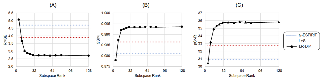
XCAT simulation results using the LR-DIP reconstruction with different subspace ranks for an acceleration factor of R=8 and trained with 10% dropout showing (A) RMSE, (B) SSIM, and (C) pSNR. For comparison, results are also shown for l₁-ESPIRiT (dotted blue line) and L+S matrix completion (dotted red line).

Figure 4 shows the effect of training with dropout while keeping the number of iterations fixed (at 20,000). The best performance was achieved using a dropout percentage of 5% to 10%. Slightly higher errors were observed when training without dropout as the network began to overfit to noise and aliasing artifacts. When using a dropout larger than 10%, the reconstruction error increased as the network failed to converge within the fixed number of iterations. As shown in Supporting Figure 2, which plots RMSE as a function of training iterations for different dropout levels, a larger dropout slowed the rate of convergence of the networks, and the best performance (lowest RMSE) was achieved using a small (5-10%) dropout level.

Figure 4.

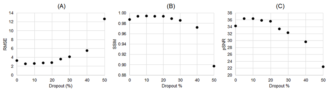
XCAT simulation results using LR-DIP trained with different dropout levels. Data were reconstructed at an acceleration factor of R=8 and using a subspace rank of 40. The x-axis shows the dropout percentage—i.e., the percentage of nodes in the spatial and temporal basis networks that were randomly disabled during each training iteration. Errors were quantified using (A) RMSE, (B) SSIM, and (C) pSNR.

Figure 5 compares errors in simulations among l₁-ESPIRIT, L+S, and LR-DIP at acceleration factors of R=6, R=8, and R=12. The LR-DIP reconstruction outperformed l₁-ESPIRiT and L+S in all cases. Larger errors were obtained at higher acceleration factors with all methods, although this effect was less pronounced for the LR-DIP reconstruction.

Figure 5.

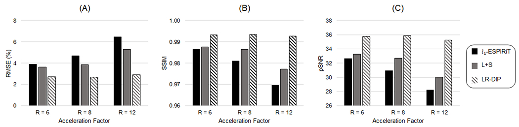
Simulation results using l₁-ESPIRiT, L+S matrix completion, and LR-DIP reconstruction methods for golden angle spiral k-space data at acceleration factors of R=6 (8 interleaves/frame), R=8 (6 interleaves/frame), and R=12 (4 interleaves/frame). The LR-DIP reconstruction employed a subspace rank of 40 and was trained with 10% dropout. Errors were quantified using (A) RMSE, (B) SSIM, and (C) pSNR.

Validation in Healthy Subjects

Supporting Figure 3 shows examples of images reconstructed using LR-DIP with different dropout levels. Images reconstructed without dropout had increased noise and residual aliasing artifacts, while dropout levels above 10% led to spatial and temporal blurring. Empirically, 10% dropout at 0.55T and 5% dropout at 1.5T were identified as providing the best image quality.

Figure 6 shows representative real-time spiral short-axis images from one healthy subject at 0.55T in diastolic and systolic cardiac phases, with corresponding movies provided in Online Resource 1. The mean reconstruction time per slice for each technique was 5 minutes for l₁-ESPIRiT, 4 minutes for L+S, and 21 minutes for LR-DIP. Images reconstructed with l₁-ESPIRiT and L+S techniques exhibited increased noise and residual aliasing artifacts compared to the LR-DIP method. Figure 7 shows real-time spiral images from a different subject at 0.55T and 1.5T, along with reference Cartesian breathheld and ECG-gated cine images at 1.5T; the corresponding movies are provided in Online Resources 2–4. Real-time scans at both field strengths enabled depiction of the myocardial wall, blood pool, and papillary muscles, with the LR-DIP reconstruction yielding visually improved noise and artifact suppression, especially at 0.55T.

Figure 6.

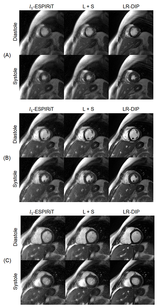
Real-time spiral bSSFP images from one healthy subject at 0.55T reconstructed with l₁-ESPIRiT, L+S matrix completion, and LR-DIP techniques. Short-axis slices are shown at (A) apical, (B) medial, and (C) basal levels of the heart and for diastolic and systolic cardiac phases (R=8, 6 interleaves/frame, 38 ms temporal resolution).

Figure 7.

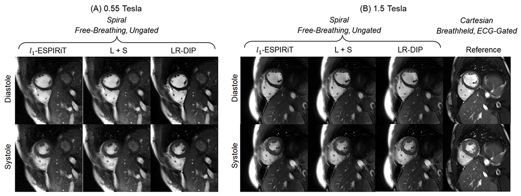
Free-breathing ungated spiral images at (A) 0.55T (R=6, 8 interleaves/frame, 38 ms temporal resolution) and (B) 1.5T (R=8, 6 interleaves/frame, 41 ms temporal resolution), as well as Cartesian breathheld and ECG-gated cine images at 1.5T, acquired in the same healthy subject. Real-time images were reconstructed with l₁-ESPIRiT, L+S matrix completion, and LR-DIP techniques.

Real-time 0.55T images in different slice orientations (short-axis, vertical long-axis, and four-chamber) are shown in Online Resource 5. The Supporting Material also contains movies with full short-axis coverage of the LV in one subject using real-time imaging with LR-DIP at 0.55T (Online Resource 6) and 1.5T (Online Resource 7) and a reference cine scan at 1.5T (Online Resource 8).

One real-time golden angle 0.55T dataset was reconstructed at different temporal resolutions of 76, 50, 38, 25, and 13 ms/frame (acceleration factors of R=4, 6, 8, 12, and 24), as shown in Figure 8 and Online Resources 9–13. Residual aliasing artifacts and blurring were observed with l₁-ESPIRiT and L+S techniques at high acceleration factors (R=12 and R=24), and these artifacts were substantially reduced using the LR-DIP reconstruction.

Figure 8.

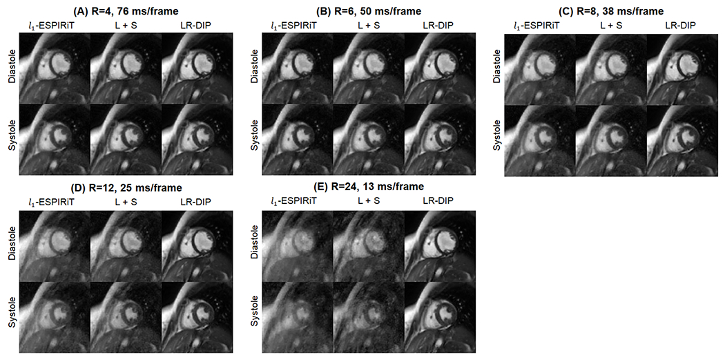
One golden angle spiral dataset collected at 0.55T was reconstructed at different temporal resolutions of (A) 76 ms (R=4, 12 interleaves/frame), (B) 50 ms (R=6, 8 interleaves/frame), (C) 38 ms (R=8, 6 interleaves/frame), (D) 25 ms (R=12, 4 interleaves/frame), and 13 ms (R=24, 2 interleaves/frame). Two image frames at end diastole and end systole are shown. Images were reconstructed using l₁-ESPIRiT, L+S matrix completion, and LR-DIP techniques. Please see Online Resources 9–13 to view these images in cine mode.

CNR measurements between blood and myocardium at 0.55T and 1.5T are plotted in Figure 9. Among the real-time sequences at 0.55T, significantly higher CNR was measured using the LR-DIP reconstruction (66.4) compared to l₁-ESPIRiT (26.9) and L+S (31.2) methods. There was no significant difference in CNR between any of the real-time methods at 1.5T and the reference cine at 1.5T, which had an average CNR of 66.1; furthermore, there was no significant difference between the reference 1.5T cine and the real-time 0.55T LR-DIP images.

Figure 9.

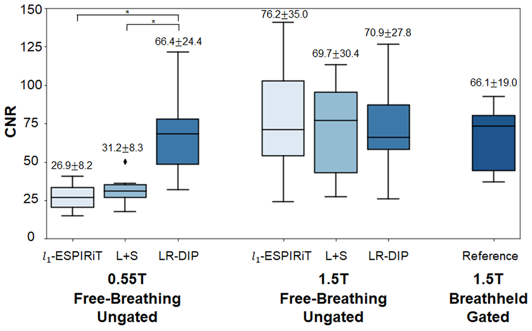
Comparison of contrast-to-noise ratio (CNR) among real-time spiral 0.55T, real-time spiral 1.5T, and breathheld/gated Cartesian cine 1.5T images. Real-time spiral images were reconstructed using l₁-ESPIRiT, L+S matrix completion, and LR-DIP techniques. CNR is reported above each boxplot as mean ± standard deviation over all subjects, with an asterisk denoting statistical significance (p<0.05).

Excellent agreement was observed on the Bland-Altman analyses comparing LV functional measurements from real-time LR-DIP images at both field strengths to the 1.5T reference cine, as shown in Figure 10. The mean bias (95% limits of agreement) for LVEF was −0.3% (−3.2%, 2.5%) at 0.55T and −0.2% (−3.0%, 2.5%) at 1.5T. For EDV, the mean bias was −1.1 mL (−14.6, 12.5) at 0.55T and −0.9 mL (−15.6, 13.8) at 1.5T. For ESV, the mean bias was 0.0 mL (−7.3, 7.4) mL at 0.55T and 0.1 mL (−7.3, 7.5) mL at 1.5T.

Figure 10.

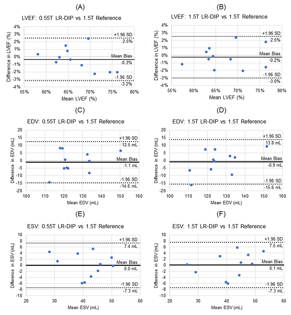
Bland-Altman plots comparing (A, B) left ventricular ejection fraction (LVEF), (C,D) left ventricular end-diastolic volume (EDV), and (E,F) left ventricular end-systolic volume (ESV) of the real-time spiral images reconstructed using the LR-DIP method at both 0.55T and 1.5T compared to the reference 1.5T cine images. The mean bias (solid line) and 95% upper and lower limits of agreement (dotted lines) are shown on each plot.

Results from the image quality rating study are shown in Figure 11. None of the differences in ratings were statistically significant. For the LR-DIP technique, average ratings were higher at 1.5T (all categories above 3.9) compared to 0.55T (all categories above 3.4); however, ratings were still above the minimum threshold of 3.0 for clinical acceptance. Compared to the 1.5T reference scans, real-time LR-DIP images received lower scores at 0.55T but similar scores at 1.5T in most categories; 1.5T LR-DIP images received slightly higher scores than the reference for visualization of LV dynamics (4.3 vs 3.9) and papillary muscle dynamics (4.3 vs 3.8). Within the same field strength, all real-time methods received similar average scores with no more than a 0.5 difference in ratings for a given category.

Figure 11.

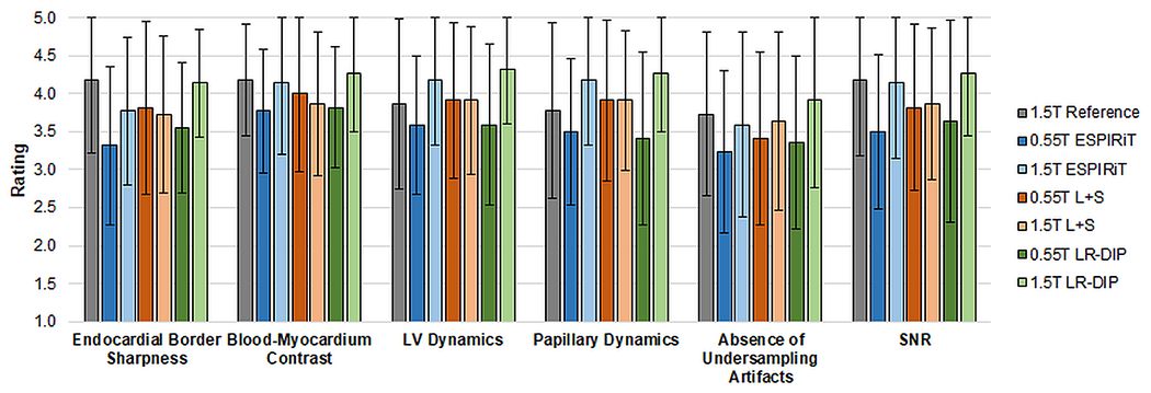
Image quality ratings from two blinded readers. The height of each bar indicates the mean rating over all subjects, and the error bars indicate the standard deviations.

Discussion

This study introduces a deep learning reconstruction for free-breathing and ungated spiral bSSFP functional cardiac imaging that combines the deep image prior framework with low-rank subspace modeling, termed a low-rank deep image prior (LR-DIP). Two u-nets separately generated spatial and temporal basis functions that were combined to yield dynamic images, with no requirements for additional training data. LV volumes and ejection fraction measurements using real-time 0.55T LR-DIP images agreed with reference cine images acquired at 1.5T. CNR measurements between blood and myocardium in real-time 0.55T LR-DIP images were significantly higher compared to 0.55T l₁-ESPIRiT and L+S images and were comparable to 1.5T reference images.

In the image quality rating study, real-time 0.55T LR-DIP images received scores above the minimum threshold of 3.0 for clinical acceptance, and real-time 1.5T LR-DIP images were scored comparably to 1.5T reference cine images. No significant differences in ratings were found between LR-DIP and the other reconstruction methods at either field strength, despite the apparent reduction in noise and undersampling artifacts seen in Figures 6–7. It should be noted that the ratings were performed using real-time images with a temporal resolution of 40 ms. As shown in Figure 8, differences in image quality between LR-DIP and the comparison reconstruction methods were more apparent at higher acceleration factors (R=12 and above), and thus image quality ratings at different temporal resolutions should be investigated in future work.

The original DIP technique used a u-net to directly output a single 2D image. This work generalizes the DIP framework for dynamic imaging by combining it with a low-rank signal approximation. One advantage of using a low-rank approach is memory efficiency, as the networks output a compressed representation of the data (i.e., a limited number of spatial and temporal basis functions) rather than generating the entire image series during each training iteration. While this study focuses on 2D dynamic imaging, the LR-DIP technique is expected to be scalable to higher-dimensional problems, including 3D and multiparametric imaging.

Most deep learning methods require training on many ground truth examples, whereas the LR-DIP technique only uses undersampled k-space data from one scan for training. Self-supervised training is beneficial for real-time CMR at 0.55T, considering that respiratory and cardiac motion and the inherently low SNR can hinder the collection of “ground truth” training datasets. However, a major disadvantage is the longer computation time compared to pre-trained deep learning techniques. Transfer learning could potentially be used to shorten the computation time by initializing the reconstruction with pre-trained network weights, which could be fine-tuned for a specific dataset by enforcing consistency with the acquired k-space data.

A general limitation of DIP methods is that networks will overfit to noise and aliasing artifacts if trained for too many iterations. This study employed dropout to avoid overfitting, although other regularization strategies can be used including early stopping, injecting random noise to the network inputs, and penalizing the l₁ or l₂ norm of the network weights. Supporting Figure 4 shows simulation results comparing different regularization strategies for the LR-DIP reconstruction, where dropout yielded the lowest errors.

Related self-supervised deep learning techniques have been proposed for real-time functional cardiac imaging at 1.5T and 3T. In the time-dependent deep image prior method, a low-dimensional manifold is mapped to latent variables using a fully-connected network, which in turn are mapped to dynamic images using an untrained convolutional network [42]. In the deep generative smoothness regularization on manifolds (SToRM) technique, both latent variables and a convolutional neural network are jointly optimized to generate dynamic images [48]. The DEBLUR technique proposed by Ahmed et al. (2022) also combines low-rank modeling with a deep image prior for dynamic cardiac imaging at 1.5T [49]. DEBLUR and LR-DIP both use untrained neural networks to generate basis functions that are combined to yield dynamic images. However, LR-DIP blindly learns basis functions and does not an employ initial estimates derived from k-space navigators or from a prior reconstruction, as used in DEBLUR.

To speed up calculation of the forward model during training, GROG was used to interpolate k-space data onto Cartesian coordinates [44]. This step allowed the use of FFT operations rather than more time-consuming NUFFT operations. For the 0.55T datasets, the average LR-DIP reconstruction time was approximately 93 minutes with NUFFT operations versus compared to 21 minutes with FFT operations (after GROG). Although GROG requires adequate coil sensitivity variations for calibration, no difficulties were encountered in this study despite the lower number of receiver coils used at 0.55T (8 channels from the spine array and 6 channels from a body phased array coil) versus 1.5T (12 channels from the spine array and 18 channels from a body phased array coil).

This work has several limitations. First, the spiral trajectory could be optimized to improve the SNR at 0.55T (e.g., by exploiting the increased T2* to lengthen the readout), which was not explored here [19]. Second, the real-time scans at 1.5T employed a relatively long TR of 5.1 ms, which can result in bSSFP banding artifacts. In this study, cardiac volume shimming was performed to mitigate banding artifacts through the heart. Third, this study employed golden angle sampling that could result in eddy current artifacts. The spiral designed for 0.55T had a lower maximum slew rate (34 mT/m/ms) than at 1.5T (130 mT/m/ms) due to the hardware constraints of the 0.55T scanner. The lower slew rate was expected to decrease eddy currents, which could be further reduced using tiny golden angle sampling. Fourth, different in-plane resolutions were employed for the real-time scans at 1.5T (1.5 x 1.5 mm²) compared to 0.55T (2.2 x 2.2 mm²). Fifth, strategies for shortening the LR-DIP reconstruction time will be addressed in future work, which may facilitate clinical translation. Sixth, only a small number of healthy subjects were enrolled in this study. Additional validation is needed in patients (especially arrhythmia patients who may benefit from free-breathing and ungated imaging) who may exhibit respiratory and cardiac motion patterns that differ from healthy subjects.

Conclusions

An initial validation in healthy subjects was presented using free-breathing and ungated spiral bSSFP imaging with a low-rank deep image prior reconstruction on a commercial 0.55T scanner, where measurements of LV volumes and ejection fraction were in good agreement with conventional breathheld and ECG-gated cine scans at 1.5T.

References

- 1.Bogaert J, Dymarkowski S, Taylor AM, Muthurangu V (2012) Clinical Cardiac MRI, 2nd ed. Springer-Verlag Berlin Heidelberg. [Google Scholar]
- 2.Pruessmann KP, Weiger M, Scheidegger MB, Boesiger P (1999) SENSE: Sensitivity encoding for fast MRI. Magn Reson Med 42:952–962. [PubMed] [Google Scholar]
- 3.Pruessmann KP, Weiger M, Boesiger P (2001) Sensitivity encoded cardiac MRI. J Cardiovasc Magn Reson 3:1–9. [DOI] [PubMed] [Google Scholar]
- 4.Griswold MA, Jakob PM, Heidemann RM, Nittka M, Jellus V, Wang J, Kiefer B, Haase A (2002) Generalized Autocalibrating Partially Parallel Acquisitions (GRAPPA). Magn Reson Med 47:1202–1210. [DOI] [PubMed] [Google Scholar]
- 5.Kellman P, Epstein FH, McVeigh ER (2001) Adaptive sensitivity encoding incorporating temporal filtering (TSENSE). Magn Reson Med 45:846–852. [DOI] [PubMed] [Google Scholar]
- 6.Breuer FA, Kellman P, Griswold MA, Jakob PM, Breuer FA, Kellman P, Griswold MA, Jakob PM (2005) Dynamic autocalibrated parallel imaging using temporal GRAPPA (TGRAPPA). Magn Reson Med 53:981–985. [DOI] [PubMed] [Google Scholar]
- 7.Uecker M, Lai P, Murphy MJ, Virtue P, Elad M, Pauly JM, Vasanawala SS, Lustig M (2014) ESPIRiT - An eigenvalue approach to autocalibrating parallel MRI: Where SENSE meets GRAPPA. Magn Reson Med 71:990–1001. [DOI] [PMC free article] [PubMed] [Google Scholar]
- 8.Tsao J, Boesiger P, Pruessmann KP (2003) k-t BLAST and k-t SENSE: Dynamic MRI With High Frame Rate Exploiting Spatiotemporal Correlations. Magn Reson Med 50:1031–1042. [DOI] [PubMed] [Google Scholar]
- 9.Huang F, Akao J, Vijayakumar S, Duensing GR, Limkeman M (2005) K-t GRAPPA: A k-space implementation for dynamic MRI with high reduction factor. Magn Reson Med 54:1172–1184. [DOI] [PubMed] [Google Scholar]
- 10.Lustig M, Donoho D, Pauly JM (2007) Sparse MRI: The application of compressed sensing for rapid MR imaging. Magn Reson Med 58:1182–1195. [DOI] [PubMed] [Google Scholar]
- 11.Feng L, Srichai MB, Lim RP, Harrison A, King W, Adluru G, Dibella EVR, Sodickson DK, Otazo R, Kim D (2013) Highly accelerated real-time cardiac cine MRI using k-t SPARSE-SENSE. Magn Reson Med 70:64–74. [DOI] [PMC free article] [PubMed] [Google Scholar]
- 12.Feng L, Grimm R, Block KT obias, Chandarana H, Kim S, Xu J, Axel L, Sodickson DK, Otazo R (2014) Golden-angle radial sparse parallel MRI: combination of compressed sensing, parallel imaging, and golden-angle radial sampling for fast and flexible dynamic volumetric MRI. Magn Reson Med 72:707–717. [DOI] [PMC free article] [PubMed] [Google Scholar]
- 13.Jung H, Park J, Yoo J, Ye JC (2010) Radial k-t FOCUSS for high-resolution cardiac cine MRI. Magn Reson Med 63:68–78. [DOI] [PubMed] [Google Scholar]
- 14.Zhao B, Haldar JP, Brinegar C, Liang Z-P (2010) Low rank matrix recovery for real-time cardiac MRI. 2010 IEEE Int. Symp. Biomed. Imaging From Nano to Macro. pp 996–999 [Google Scholar]
- 15.Lingala SG, Hu Y, Dibella E, Jacob M (2011) Accelerated dynamic MRI exploiting sparsity and low-rank structure: k-t SLR. IEEE Trans Med Imaging 30:1042–1054. [DOI] [PMC free article] [PubMed] [Google Scholar]
- 16.Pedersen H, Kozerke S, Ringgaard S, Nehrke K, Won YK (2009) K-t PCA: Temporally constrained k-t BLAST reconstruction using principal component analysis. Magn Reson Med 62:706–716. [DOI] [PubMed] [Google Scholar]
- 17.Otazo R, Candès E, Sodickson DK (2015) Low-rank plus sparse matrix decomposition for accelerated dynamic MRI with separation of background and dynamic components. Magn Reson Med 73:1125–36. [DOI] [PMC free article] [PubMed] [Google Scholar]
- 18.Wang D, Smith DS, Yang X (2020) Dynamic MR image reconstruction based on total generalized variation and low-rank decomposition. Magn Reson Med 83:2064–2076. [DOI] [PMC free article] [PubMed] [Google Scholar]
- 19.Campbell-Washburn AE, Ramasawmy R, Restivo MC, Bhattacharya I, Basar B, Herzka DA, Hansen MS, Rogers T, Patricia Bandettini W, McGuirt DR, Mancini C, Grodzki D, Schneider R, Majeed W, Bhat H, Xue H, Moss J, Malayeri AA, Jones EC, Koretsky AP, Kellman P, Chen MY, Lederman RJ, Balaban RS (2019) Opportunities in interventional and diagnostic imaging by using high-performance low-field-strength MRI. Radiology 293:384–393. [DOI] [PMC free article] [PubMed] [Google Scholar]
- 20.Simonetti OP, Ahmad R (2017) Low-Field Cardiac Magnetic Resonance Imaging: A Compelling Case for Cardiac Magnetic Resonance’s Future. Circ Cardiovasc Imaging 10:e005446. [DOI] [PMC free article] [PubMed] [Google Scholar]
- 21.Hoult DI, Phil D (2000) Sensitivity and power deposition in a high-field imaging experiment. J Magn Reson Imaging 12:46–67. [DOI] [PubMed] [Google Scholar]
- 22.Strach K, Naehle CP, Mühlsteffen A, Hinz M, Bernstein A, Thomas D, Linhart M, Meyer C, Bitaraf S, Schild H, Sommer T (2010) Low-field magnetic resonance imaging: Increased safety for pacemaker patients? Europace 12:952–960. [DOI] [PubMed] [Google Scholar]
- 23.Bandettini WP, Shanbhag SM, Mancini C, McGuirt DR, Kellman P, Xue H, Henry JL, Lowery M, Thein SL, Chen MY, Campbell-Washburn AE (2020) A comparison of cine CMR imaging at 0.55 T and 1.5 T. J Cardiovasc Magn Reson 22:37. [DOI] [PMC free article] [PubMed] [Google Scholar]
- 24.Srinivasan S, Ennis DB (2015) Optimal flip angle for high contrast balanced SSFP cardiac cine imaging. Magn Reson Med 73:1095–1103. [DOI] [PubMed] [Google Scholar]
- 25.Restivo MC, Ramasawmy R, Bandettini WP, Herzka DA, Campbell-Washburn AE (2020) Efficient spiral in-out and EPI balanced steady-state free precession cine imaging using a high-performance 0.55T MRI. Magn Reson Med 84:2364–2375. [DOI] [PMC free article] [PubMed] [Google Scholar]
- 26.Tian Y, Cui SX, Lim Y, Lee NG, Zhao Z, Nayak KS (2022) Contrast-optimal simultaneous multi-slice bSSFP cine cardiac imaging at 0.55 T. Magn Reson Med. doi: 10.1002/mrm.29472 [DOI] [PMC free article] [PubMed] [Google Scholar]
- 27.Fyrdahl A, Seiberlich N (2022) Real-time Cardiac MRI at 0.55T using through-time spiral GRAPPA. Proc. 31st Annu. ISMRM. p 1843 [Google Scholar]
- 28.Tian Y, Lim Y, Nayak KS (2022) Real-Time Water Fat Imaging at 0.55T with Spiral Out-In-Out-In Sampling. Proc. 31st Annual ISMRM. p 317 [Google Scholar]
- 29.Küstner T, Fuin N, Hammernik K, Bustin A, Qi H, Hajhosseiny R, Masci PG, Neji R, Rueckert D, Botnar RM, Prieto C (2020) CINENet: deep learning-based 3D cardiac CINE MRI reconstruction with multi-coil complex-valued 4D spatio-temporal convolutions. Sci Rep 10:1–13. [DOI] [PMC free article] [PubMed] [Google Scholar]
- 30.Sandino CM, Lai P, Vasanawala SS, Cheng JY (2021) Accelerating cardiac cine MRI using a deep learning-based ESPIRiT reconstruction. Magn Reson Med 85:152–167. [DOI] [PMC free article] [PubMed] [Google Scholar]
- 31.El-Rewaidy H, Fahmy AS, Pashakhanloo F, Cai X, Kucukseymen S, Csecs I, Neisius U, Haji-Valizadeh H, Menze B, Nezafat R (2021) Multi-domain convolutional neural network (MD-CNN) for radial reconstruction of dynamic cardiac MRI. Magn Reson Med 85:1195–1208. [DOI] [PubMed] [Google Scholar]
- 32.Jaubert O, Montalt-Tordera J, Knight D, Coghlan GJ, Arridge S, Steeden JA, Muthurangu V (2021) Real-time deep artifact suppression using recurrent U-Nets for low-latency cardiac MRI. Magn Reson Med 86:1904–1916. [DOI] [PMC free article] [PubMed] [Google Scholar]
- 33.Shen D, Ghosh S, Haji-Valizadeh H, Pathrose A, Schiffers F, Lee DC, Freed BH, Markl M, Cossairt OS, Katsaggelos AK, Kim D (2021) Rapid reconstruction of highly undersampled, non-Cartesian real-time cine k-space data using a perceptual complex neural network (PCNN). NMR Biomed 34:e4405. [DOI] [PMC free article] [PubMed] [Google Scholar]
- 34.Hauptmann A, Arridge S, Lucka F, Muthurangu V, Steeden JA (2019) Real-time cardiovascular MR with spatio-temporal artifact suppression using deep learning-proof of concept in congenital heart disease. Magn Reson Med 81:1143–1156. [DOI] [PMC free article] [PubMed] [Google Scholar]
- 35.Morales MA, Assana S, Cai X, Chow K, Haji-Valizadeh H, Sai E, Tsao C, Matos J, Rodriguez J, Berg S, Whitehead N, Pierce P, Goddu B, Manning WJ, Nezafat R (2022) An inline deep learning based free-breathing ECG-free cine for exercise cardiovascular magnetic resonance. J Cardiovasc Magn Reson 24:47. [DOI] [PMC free article] [PubMed] [Google Scholar]
- 36.Ulyanov D, Vedaldi A, Lempitsky V (2018) Deep Image Prior. Proc. IEEE Comput. Soc. Conf. Comput. Vis. Pattern Recognit. IEEE Computer Society, pp 9446–9454 [Google Scholar]
- 37.Chakrabarty P, Maji S (2019) The spectral bias of the deep image prior. arXiv Prepr. arXIV1912.08905 [Google Scholar]
- 38.Laves M-H, Tölle M, Ortmaier T (2020) Uncertainty Estimation in Medical Image Denoising with Bayesian Deep Image Prior. Med Image Comput Comput Assist Interv. doi: 10.48550/ARXIV.2008.08837 [DOI] [Google Scholar]
- 39.Lin YC, Huang HM (2020) Denoising of multi b-value diffusion-weighted MR images using deep image prior. Phys Med Biol. doi: 10.1088/1361-6560/ab8105 [DOI] [PubMed] [Google Scholar]
- 40.Jafari R, Spincemaille P, Zhang J, Nguyen TD, Luo X, Cho J, Margolis D, Prince MR, Wang Y (2021) Deep neural network for water/fat separation: Supervised training, unsupervised training, and no training. Magn Reson Med 85:2263–2277. [DOI] [PMC free article] [PubMed] [Google Scholar]
- 41.Hamilton JI (2022) A Self-Supervised Deep Learning Reconstruction for Shortening the Breathhold and Acquisition Window in Cardiac Magnetic Resonance Fingerprinting. Front Cardiovasc Med 9:928546. [DOI] [PMC free article] [PubMed] [Google Scholar]
- 42.Yoo J, Jin KH, Gupta H, Yerly J, Stuber M, Unser M (2021) Time-Dependent Deep Image Prior for Dynamic MRI. IEEE Trans Med Imaging 40:3337–3348. [DOI] [PubMed] [Google Scholar]
- 43.Fessler J, Sutton B (2003) Nonuniform fast Fourier transforms using min-max interpolation. IEEE Trans Signal Process 51:560–574. [Google Scholar]
- 44.Seiberlich N, Breuer FA, Blaimer M, Barkauskas K, Jakob PM, Griswold MA (2007) Non-Cartesian data reconstruction using GRAPPA operator gridding (GROG). Magn Reson Med 58:1257–1265. [DOI] [PubMed] [Google Scholar]
- 45.Segars WP, Sturgeon G, Mendonca S, Grimes J, Tsui BMW (2010) 4D XCAT phantom for multimodality imaging research. Med Phys 37:4902–4915. [DOI] [PMC free article] [PubMed] [Google Scholar]
- 46.Winkelmann S, Schaeffter T, Koehler T, Eggers H, Doessel O (2007) An optimal radial profile order based on the Golden Ratio for time-resolved MRI. IEEE Trans Med Imaging 26:68–76. [DOI] [PubMed] [Google Scholar]
- 47.Yushkevich PA, Piven J, Hazlett HC, Smith RG, Ho S, Gee JC, Gerig G (2006) User-guided 3D active contour segmentation of anatomical structures: significantly improved efficiency and reliability. Neuroimage 31:1116–1128. [DOI] [PubMed] [Google Scholar]
- 48.Zou Q, Ahmed AH, Nagpal P, Kruger S, Jacob M (2021) Dynamic Imaging Using a Deep Generative SToRM (Gen-SToRM) Model. IEEE Trans Med Imaging 40:3102–3112. [DOI] [PMC free article] [PubMed] [Google Scholar]
Associated Data
This section collects any data citations, data availability statements, or supplementary materials included in this article.