

Abstract
We present a methodology to image and quantify the shear elastic modulus of three dimensional (3D) breast tissue volumes held in compression under conditions similar to those of a clinical mammography system. Tissue phantoms are made to mimic the ultrasonic and mechanical properties of breast tissue. Stiff lesions are created in these phantoms with size and modulus contrast values, relative to the background, that are within the range of values of clinical interest. A two dimensional ultrasound system, scanned elevationally, is used to acquire 3D images of these phantoms as they are held in compression. From two 3D ultrasound images, acquired at different compressed states, a three dimensional displacement vector field is measured. The measured displacement field is then used to solve an inverse problem, assuming the phantom material to be an incompressible, linear elastic solid, to recover the shear modulus distribution within the imaged volume. The reconstructed values are then compared to values measured independently by direct mechanical testing.
1. Introduction
Ultrasound elasticity imaging, or elastography, offers an attractive adjunct to film and digital mammography for breast cancer screening applications. Among the various approaches to elastography, perhaps the most common is that pioneered by Ophir and coworkers (Ophir et al. 1991). This technique is based on ultrasound tracking of quasistatic breast compression to generate strain images. Several clinical studies (Garra et al. 1997, Hall et al. 2003, Regner et al. 2006, Giuseppetti et al. 2005, Itoh et al. 2006, Thomas et al. 2006, Zhi et al. 2007, Burnside et al. 2007, Bamber et al. 2002) have demonstrated that the resulting strain images typically improve the diagnostic accuracy over ultrasound alone. While these studies all use 2D ultrasound, there is a trend toward 3D ultrasound imaging (Weismann 2005), including 3D strain imaging (Lindop et al. 2006, Krueger et al. 1998, Lorenz et al. 1999, Treece et al. 2008).
Beyond the ability to create 3D images, three dimensional ultrasound elastography offers several potential benefits over 2D ultrasound elastography. Among these is the ability to track motion in the elevation direction. Another is the ability to use physical constraints, e.g. tissue incompressiblity, to improve motion tracking from frame-to-frame. Both of these are used here. One of the most significant advantages of 3D imaging, potentially, is the obviation of 2D model simplifying assumptions when reconstructing modulus distributions.
One step beyond strain imaging is elastic modulus imaging. This involves solving a (non-trivial) inverse problem to determine the elastic modulus distribution that is consistent with the measured strain field. This was pioneered by Kallel & Bertrand (1996), Raghavan & Yagle (1994) and Skovoroda et al. (1995), and strain and modulus images were quantitatively compared in Doyley et al. (2005). More recent approaches can be found in Doyley et al. (2000), Oberai et al. (2004) and Gokhale et al. (2004). In all these cases, 2D ultrasound elastography was used, and so only planar displacement data was available. As a result, some simplifying assumption, e.g. plane stress or plane strain, was required. Other authors (Steele et al. 2000, Sumi 2006) argue persuasively and demonstrate that such 2D approximations can lead to significant error when they are violated.
Here we describe the results of a study designed to evaluate the potential to reconstruct the 3D modulus distribution in tissue mimicking phantoms from ultrasound measured quasistatic compressions. The experimental protocol was designed to mimic the use of ultrasound elasticity imaging as an adjunct to mammographic breast screening. It utilizes a linear ultrasound array scanned mechanically in the elevation direction to collect a 3D volume of data. The sample is held between a pair of comparatively rigid compression plates, and the ultrasound is introduced through a window in one of the plates.
The phantoms used in our study exhibited a variety of inclusion sizes (~5 mm-13 mm) and contrasts (~1–3) and were set in a background with inhomogeneous (layered) properties. Other novel features of the study include attention to the role of boundary conditions in the reconstruction (Barbone & Bamber 2002) and a novel 3D displacement estimation method, which will be introduced in this paper but described in detail elsewhere.
The technique used here to reconstruct the elastic modulus from the measured displacement fields was adapted from Oberai et al. (2003) and Oberai et al. (2004). This is based on an optimization approach. That is, we seek the modulus distribution that, when used in a forward model to compute a predicted displacement field, gives the best match to the measured displacement fields. The optimization method chosen here utilizes the BFGS (Broyden Fletcher Goldfarb Shanno (Nocedal 1980)) method to minimize this difference in displacement fields. This quasi-Newton algorithm requires only the functional value and the first derivative (i.e. the gradient) of the functional be calculated explicitly at each iteration. The adjoint method is used to efficiently calculate the gradient (Oberai et al. 2003, Oberai et al. 2004).
Section 2 presents our methods for phantom construction, the design of the scanning apparatus, the 3D ultrasound imaging protocol and the techniques used to independently measure the phantom’s mechanical properties. Section 3.1 outlines the image registration based algorithm used to measure the displacement vector fields from the 3D ultrasound images. This technique was developed as an alternative to standard cross-correlation based measurement techniques. Section 3.2 gives our formulation of the inverse problem and the assumptions necessary for modulus reconstruction. Section 4 presents the results from the displacement estimations and phantom reconstructions. Lastly, in Sections 5 and 6 we discuss the implications of our results and the future directions of this work. Appendix A outlines the simulation studies used to determine the appropriate parameter values necessary for the displacement estimation and reconstruction.
2. Experimental Methods
2.1. Phantom manufacture
The phantoms used in this study were a mixture of 300 bloom gelatin and silica made to mimic the acoustic and elastic properties of soft tissue. Approximately 2% by mass concentration of silica particles were suspended in gelatin as scatterers to reproduce a full speckle image. The relative phantom stiffness was modified by varying the gelatin concentration. Phantoms were cuboid in shape with a base of 60 mm by 60 mm and a height of 50 mm. The background material of the phantoms was made with an 8% by mass concentration gelatin solution. Close to the center of the phantom, cylindrical inclusions of varying size were made to mimic the elevated stiffness of tumors relative to healthy tissue with 10%, 12% or 16% by mass concentration gelatin solutions. The sizes of the inclusions were varied by changing the size of the mold used to pour the gelatin. Three cylindrical inclusion sizes were tested with volumes 1280 mm3 (12.8 mm in diameter and 10 mm in height), 390 mm3 (7.94 mm in diameter and 8 mm in height) and 87 mm3 (4.80 mm in diameter and 5 mm in height). A bottom layer (approximately 10 mm of additional height), with an elevated stiffness typically matching that of the inclusion, was also added to each phantom. Prior to each additional gelatin pour of a given phantom, the previous gelatin layer was flushed with warm water to aid adhesion. A picture of the phantom is shown in Figure 2.1. In this picture, regions with elevated stiffness appear darker than the background which is at a lower stiffness. A quantity of each type of gelatin solution used in the phantom was poured into several (typically 4–5 samples total per gelatin pour) cylindrical cake molds (15 mm diameter×10 mm height) for independent stiffness calibrations.
Three inclusion sizes and three modulus contrasts were investigated. They were selected to identify the spatial and contrast resolution of these techniques. The modulus contrasts lie at the lower limit of clinical interest in detecting breast cancer, and can be considered as a stringent test of the proposed methods. The smallest inclusion used is at the limit of the manufacturing capabilities and once again at the lower limit of current clinical interest. Seven inclusions total were tested. Only the high contrast inclusion was tested for the largest volume.
2.2. Stiffness calibration
The calibration of each individual gelatin pour was performed using a Q800 Dynamic Mechanical Analysis machine (TA instruments, New Castle, DE 19720). To determine the elastic modulus of each sample, an unconfined compression test was used to measure the force/displacement relationship of each sample in the range of 1–10% strain. During each test, the samples were visually inspected for signs of slipping, which was minimized by maintaining a dry surface contact between the gel and the roughened platens of the device. These boundary conditions, however, produce a nonuniform stress field in the samples which, in turn, cause the measured force-displacement slope to deviate from the actual modulus measurement by a multiplicative constant. A numerical simulation using FlexPDE (PDE Solutions Inc., Spokane Valley, WA 99206) was performed, for the given size and geometry of these gel samples, to determine this constant and correct our measured values. Each sample was kept at refrigerator temperature (approx. 4°C) up to the point at which it was tested. During storage, all samples were kept in an air tight container to limit water loss. The samples for each phantom were tested within 24 hours of the corresponding phantom imaging experiment. The duration of the calibration measurements were approximately 1 minute per sample.
2.3. Imaging setup
The experimental setup for the phantom experiments was developed using a two dimensional ultrasound scanner (Analogic AN2300) and is shown in Figure 2. The Analogic AN2300 (Analogic Corp., 8 Centennial Drive, Peabody, MA 01960) allows for full radio frequency (RF) image capture. The transducer used was a 9.5 MHz center frequency, linear array (Type 8805)(B&K, Mileparken 34, DK-2730 Herlev, Denmark), with a usable bandwidth (stated by the manufacturer) from 5–12 MHz.
Figure 2.
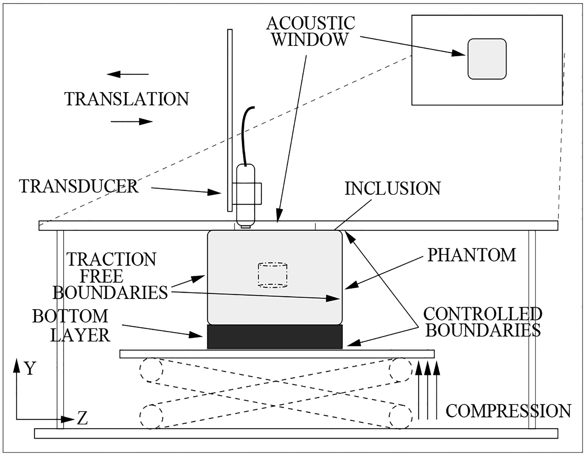
Compression and Imaging Experimental Setup.
The phantoms were held in place by two plates on the bottom and top (see Figure 2). The top plate has a section removed to serve as an acoustic window. When the top plate was brought into contact with the phantom, the window forms a small well which, when filled with water, allows non-contact acoustic coupling between the transducer and the phantom. The transducer was scanned elevationally in 0.14 mm steps across this window, using a Newport stepper motor (Newport Corp., 1791 Deere Avenue, Irvine, CA) with micrometer accuracy, to obtain a 3D image. After an initial image was obtained, a small compressive strain was applied (typically ~1–2%), and then a second post deformation image was obtained. The spatial location of the pixels in the axial direction () was found using the sampling frequency of the transducer (40 MHz) and an assumed sound speed of 1535 m/s. The lateral and elevational locations were determined by the transducer element spacing and the stepper motor control, respectively. The scanned volume measured ≈67.0 mm×30.3 mm×26.9 mm in the axial, lateral, and elevational directions, respectively. The duration of the imaging experiment was approximately 1/2 hour for each phantom, however, the process has not yet been optimized for time.
3. Analysis Methods
The analysis methods used to create the elastic shear modulus images are comprised of two optimization algorithms. The first algorithm is an image registration based technique which measures the 3D displacement vector field, from a pair of 3D pre- and post-deformation ultrasound images acquired using the protocol outlined in Section 2. The second algorithm is a constrained optimization technique which seeks to find a shear modulus distribution which is most consistent with the observed displacement field. This algorithm requires the assumption of a linear elastic, isotropic, incompressible material model. These algorithms are briefly described in the following sections.
3.1. Displacement estimation
Fundamental to the process of elasticity imaging is the ability to measure physically accurate displacements from image sets of deforming tissues or phantoms. The primary assumption of this measurement technique is that the deformation required to map one image to another results directly from the underlying tissue motion alone. That is, suppose we are given the functions and , which are spatial distributions of the scalar image intensities. Here, represents an initial, predeformation image of some tissue and represents the image of the same tissue after it has undergone some mechanical perturbation. Then it is assumed that the relation between the images can be approximated as:
| (1) |
Here, the displacement field is the underlying tissue motion. In effect, this displacement field acts as a nonlinear scaling of the position vector defining the intensities of the original image. In practice, we approximate using finite element basis functions defined over a prescribed mesh.
The image registration algorithm used in this study is an iterative optimization technique which minimizes the image intensity difference of the pre- and post-deformation images with respect to the measured displacement. Using an optimization technique such as this allows for the implementation of regularization and other constraints to decrease estimate variance and avoid erroneous results. It also allows for a higher order interpolation of the underlying displacement functions. Using a linear interpolation of , for instance, reduces the effect of image decorrelation in the displacement estimates by accounting for all locally affine motions within each element. One disadvantage of the optimization algorithm in comparison with cross-correlation based techniques is its rather large computational cost.
The functional minimized in each measurement of the displacement field is:
| (2) |
In this functional, and are the pre- and post-deformation images, respectively, and is the spatial domain of interest. The term includes the regularization and constraint terms used in this implementation. This functional is minimized using a Gauss-Newton method which requires both the gradient and an approximation to the Hessian of this functional with respect to the function .
In this algorithm, the function and its variants are discretized using finite element, trilinear interpolation function approximations. The integration calculations use a three dimensional midpoint rule and the images are interpolated at each integration point using cubic Lagrange polynomials. The integration calculations were parallelized to improve the speed of the iterations (OpenMP) and the equations were solved using a parallelized linear solver (PARDISO) (Intel Corp., 2200 Mission College Blvd., Santa Clara, CA 95052) (Schenk & Gartner 2004, Schenk & Gartner 2006).
To limit the effect of noise it is often assumed that the solution, in this case , is smooth (i.e. has a bounded norm) and thus another term is added to the functional which penalizes noise in the measurement. The implementation of the above algorithm uses an semi-norm regularization to penalize large gradients in :
| (3) |
Here, the scalar determines the amount or strength of the regularization (smoothing) relative to the functional. The appropriate value of will depend on the images used, the expected signal to noise ratio and the magnitude of the strain. Therefore this value is system and protocol specific and needs to be determined for each system independently.
One advantage of capturing a full 3 component 3D vector data set is that the a priori knowledge that breast tissue is an incompressible material may be used to further constrain the displacements measured from these image pairs. To implement this, another term is added to the functional of equation (2) which penalizes nonzero volume change over each finite element:
| (4) |
The relative strength of the incompressibility term will be determined by the magnitude of the parameter. This term, however, is not appropriately considered a regularization term. Rather, it is a constraint that is being enforced via a penalty. Ideally and naively, therefore, could be taken to infinity. In practice however, is determined as the highest value after which no improvement in the measured is observed. The form of equation (4) was chosen to avoid mesh locking associated with pointwise penalties of volume change (Hughes 1999). Examples of calculated displacement fields will be shown in Section 4.1.
In this study, we follow a systematic procedure for the selection of the processing parameters, and , as described in Appendix A.
3.2. Inverse formulation: theory
The last step in the process of elasticity imaging is to use the measured displacement fields (i.e. all 3 vector components) as input to an inverse problem to determine the mechanical properties of the underlying material. A necessary assumption about the input to this inverse problem is that the tissue behaviour can be accurately predicted by a mathematical model. In this regard we use a linear elastic, (nearly) incompressible, single phase, isotropic model to predict the tissue behaviour. The constraint equations used in the inverse problem, combining the constitutive equations of the model and the conservation of linear momentum, are:
| (5) |
and
| (6) |
Here, is (approximately) the hydrostatic pressure, and are the Lamé coefficients, and is the second order identity tensor. In this work, is taken to be constant and large (i.e. ). It is determined by specifying the Poisson’s ratio , and evaluating . The reference value of is unity, which is also the lower limit of for a given inversion. The boundary conditions are specified in the following form:
| (7) |
and
| (8) |
At each point on the boundary and in each spatial direction , either the traction or the displacement must be prescribed (i.e. and ).
For our analysis, equations (5–8) are discretized and solved using (almost) standard trilinear finite elements. The Lamé parameters, and are interpolated as piece-wise constant, i.e. constant over each element. Nearly incompressible behaviour is addressed with selective reduced integration, which, on the regular meshes used here, is exactly equivalent to a mixed method with piece-wise constant pressure interpolation (Hughes 1999). The finite element mesh used to represent the displacement field in the inverse problem is identical to that used in image matching.
The underlying idea of our inverse formulation is to find a modulus distribution which is most consistent with the observed displacement field. That is, we try to minimize the difference between the measured displacements and the displacements predicted by the constraint equations (Oberai et al. 2003, Oberai et al. 2004). The optimization functional is given by:
| (9) |
Here is a second order tensor whose diagonal entries represent a weighted contribution of each of the displacement components to the functional and whose off diagonal entries are zero. This allows for the inversion to account for the difference in the accuracy of the displacement estimates in each direction. The term is a regularization term, discussed below. A BFGS optimization method was used to minimize this functional and the adjoint method is used to efficiently calculate the gradient (Oberai et al. 2003, Oberai et al. 2004).
The regularization used in our algorithm is based on a total variation diminishing (TVD) type of penalty term. We chose a TVD regularization because this type of regularization is well suited to data which exhibits discontinuous jumps in the underlying modulus distributions. That is, TVD regularization tends to penalize high oscillations in the solutions (i.e. noise) while allowing lower frequency jumps (Vogel 2002). The standard TVD regularization functional term of a scalar function is:
| (10) |
In practice, the singularity in the absolute value function must be smoothed. The computational implementation of equation (10) chosen here is:
| (11) |
The constant is user selected and “small” in an appropriate sense. The differential of this functional is:
| (12) |
With piecewise constant interpolation as used here, equation (12) cannot be used directly; the gradients must be interpreted in a generalized sense. Carrying this out leads to the following, in terms of jumps in across element boundaries:
| (13) |
Here, is the modulus value of the element of integration, is that of a bordering element, is the area of the surface joining these two elements and is a number between 3 and 6 defining the number of surfaces which element shares with neighboring elements.
As in the image registration code, the integration required to calculate the stiffness matrix and the right hand side vectors of the elasticity equations, as well as the gradient and function evaluations were parallelized to further improve the speed of each iteration (OpenMP). A parallelized linear solver (PARDISO) is also used to solve each forward problem.
A single iteration of this 3D reconstruction algorithm (2 matrix inversions) took ~200 seconds (parallelized on 9 processors). A 2D reconstruction iteration, with a comparable axial/lateral mesh size, takes ~0.25 seconds (parallelized on 2 processors). The 3D algorithm typically took ~40 iterations to reach the convergence criteria defined above.
4. Results
4.1. Displacement estimates
For each reconstructed image the displacement measurement and subsequent modulus reconstruction was performed using a uniform mesh of finite elements of size 0.6 mm×1.0 mm×0.6 mm in the and directions, respectively (40×60×40 elements). For the displacement estimation algorithm, the regularization and incompressibility parameters were set to and , respectively. These values were selected from a series of separate tests performed on synthetic data. These tests are described in Appendix A. An initial guess for was created based on the overall strain applied during the image acquisition. The termination point of the displacement matching iterations was found in a two step process. First, several iterations and manual updates were performed on the displacement initialization guess to ensure the displacement estimate avoided any local minima. The algorithm was then allowed to iterate until remained relatively constant with iterations, to ensure that it had fully converged. The accuracy of the registration was monitored within each element by computing the normalized norm of the difference in the motion compensated image pairs inside each element. That is, for every element “e”, the metric:
| (14) |
was evaluated. In all cases, the mean value of over the image was less than 0.2. A typical displacement estimate is shown in Figure 3. Displacement estimation typically took on the order of several hours to converge on the measurement for each image pair processed. For comparison purposes, the axial and lateral displacement components in a central slice are shown here along with example displacements measured with a simple 2D cross correlation method.
Figure 3.
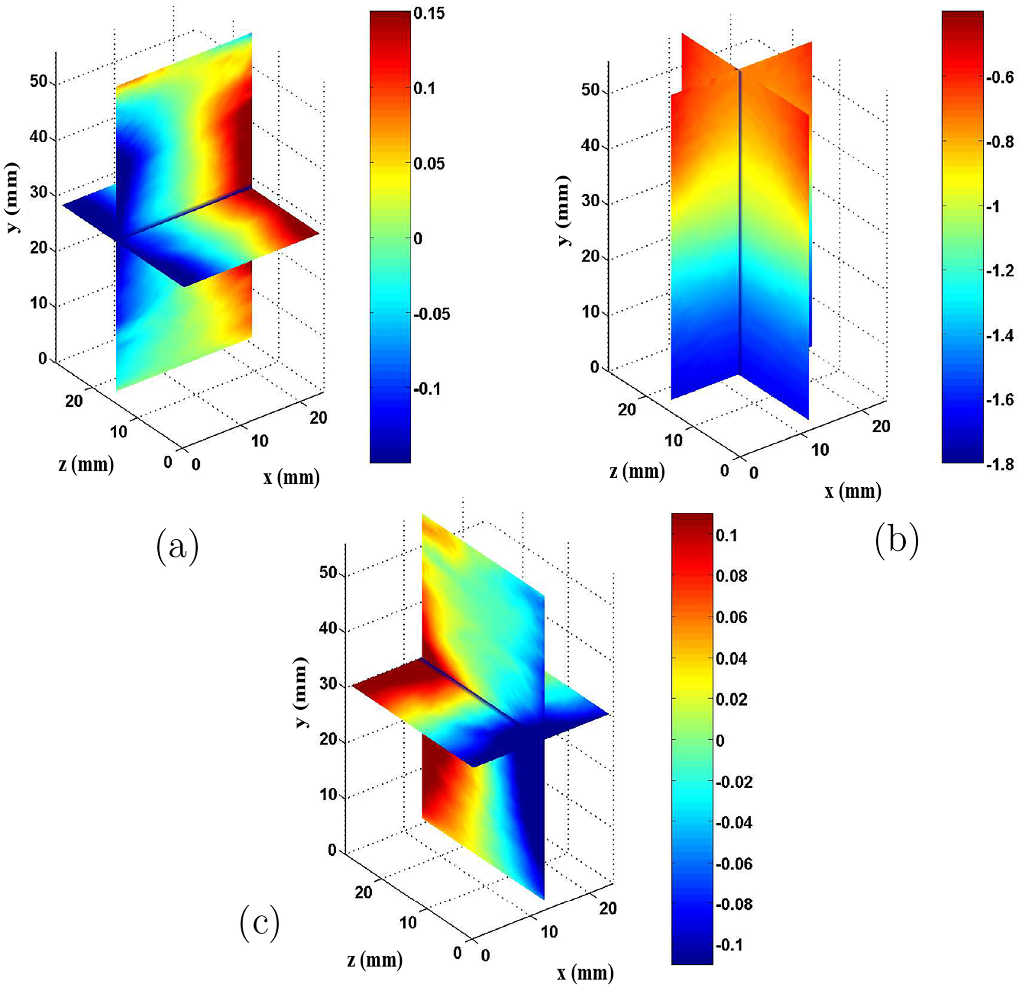
Displacement estimates from ultrasound phantom images (mm). (a) Lateral displacement (-direction), (b) axial displacement (-direction), (c) elevational displacement (-direction).
4.2. Modulus reconstructions
The measured displacements were then input to the inverse algorithm, using the same mesh size and location. The boundary conditions used to compute the predicted displacement field were such that the sides of the reconstructed volume (i.e. the and boundary surfaces) were assumed to have zero normal traction ( on and ). The remaining boundary conditions were specified displacements (Dirichlet conditions). A Poisson’s ratio of 0.4995 and a TVD regularization parameter of were used in the reconstructions. The weighting matrix was set such that the diagonal components , and and the off diagonal components were set to 0. The type of boundary conditions and the value of the parameters , and were selected from a series of independent tests performed on synthetic data, as described in Appendix A. The initial guess of was homogeneous with value 1 and the iterations were terminated at first iteration for which the value . The functional value, used to determine the stopping criterion, was calculated from the displacement matching term alone, without the regularization term. Figure 5 shows slices through the volume of a typical modulus reconstruction.
Figure 5.
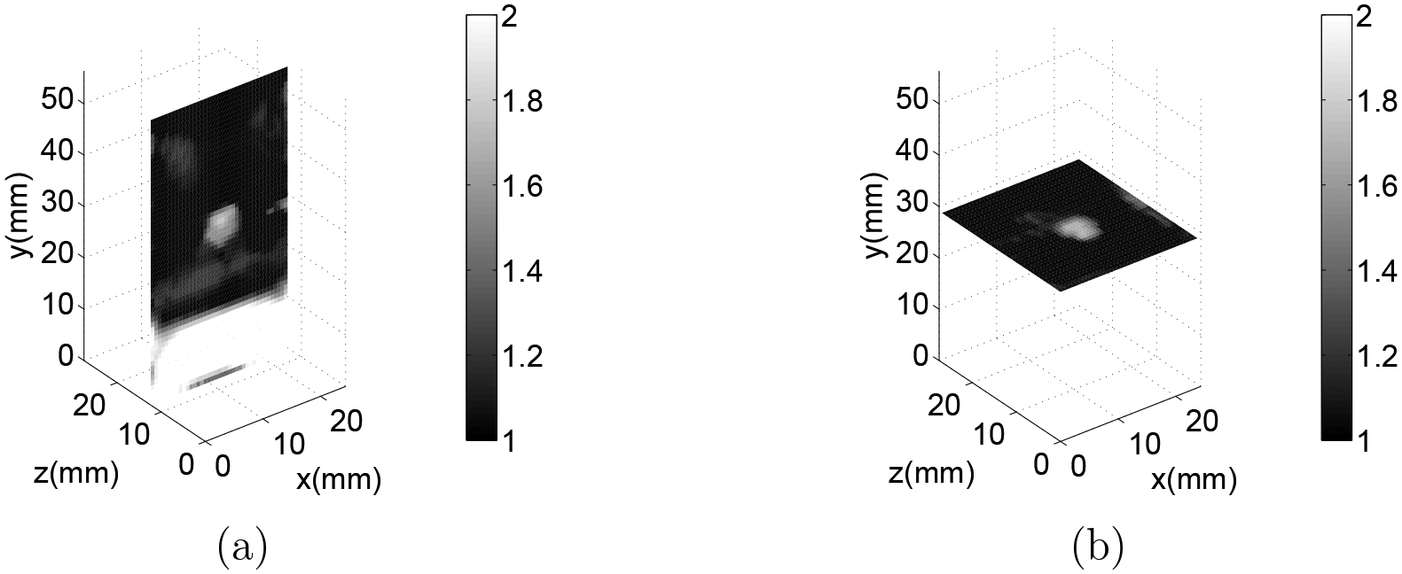
(a) slice of 3D modulus reconstruction for a small inclusion with a 12% by mass gelatin concentration through the center of the inclusion. (b) slice of 3D modulus reconstruction for this same inclusion through the center of the inclusion. Note that the cylindrical shape of this ~5 mm inclusion is apparent.
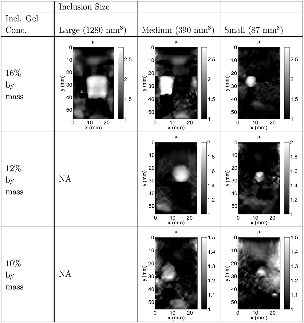
Table 1 shows the values of the recovered modulus contrasts of each inclusion type tested as well as the expected modulus contrast values for each inclusion calculated from the independent mechanical tests. In this table, is the reference modulus contrast of the independently measured gelatin samples for the inclusion relative to the background, is the recovered or reconstructed contrast reported for the inclusion relative to the background, is the strain contrast measured in the background relative to the inclusion and is the ratio of the reconstructed inclusion volume to the expected volume of the inclusion when it was made. To evaluate the recovered contrast and size of the inclusion in the reconstructions, the half maximum of the inclusion was determined by inspection. The average modulus of the elements with modulus values above the half maximum was evaluated and designated as the recovered inclusion modulus value. The volume of the inclusion was found by counting the number of elements with modulus values greater than the half maximum and multiplying this number by the volume of each element. Using the axial strain field, created from the measured displacements, a value of the average strain in the inclusion and in a homogeneous portion of the background were also calculated. Table 2 shows the central slice from the modulus reconstruction images of each of the seven reconstructions reported for the various inclusion sizes and contrasts.
Table 1.
Reconstructed modulus contrast accuracy reported for the inclusion sizes and gelatin concentrations.
| Inclusion Size | |||
|---|---|---|---|
| Inc. Gel Conc. | Large (1280 mm3) | Medium (390 mm3) | Small (87 mm3) |
| 16% by mass | |||
| . | |||
| 12% by mass | |||
| NA | |||
| 10% by mass | |||
| NA | . | ||
Table 2.
Reconstructed modulus image slices (the central slice from each phantom reconstruction) reported for their respective inclusion sizes and gelatin concentrations.
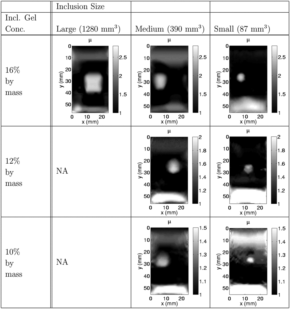
|
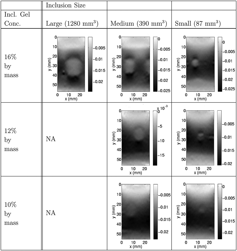
For comparison, Table 4 shows the central slice from the strain images of each of the seven reconstructions reported for the various inclusion sizes and contrasts. Table 3 demonstrates the effect of the choice of boundary conditions on the reconstructed modulus images. This was accomplished by repeating all the reconstructions reported in Table 2 with displacement (Dirichlet) boundary conditions on all surfaces. All other parameters of the reconstruction (regularization, convergence criterion etc.) were kept unchanged. This lead to the reconstructions shown in Table 3. We observe that these reconstructions are not as accurate as those reported with traction boundary conditions. For example, they completely fail to represent the inhomogeneity of the background medium.
Table 4.
Axial strain image slices (the central slice from each phantom reconstruction) reported for their respective inclusion sizes and gelatin concentrations.
|
Table 3.
Reconstructed modulus image slices (the central slice from each phantom reconstruction), using all Dirichlet boundary conditions, reported for their respective inclusion sizes and gelatin concentrations.
|
We use several benchmarks by which we evaluate our reconstructions. The first is a qualitative comparison to the strain images, which may be regarded as a “gold standard” in quasistatic elastography. A second is a comparison of the reconstructed inclusion contrast to the calibration measurements of the separate samples. A third is a geometric evaluation of the size of the inclusion and the presence of the layered background. We discuss these now.
The current standard in elastography practice is strain imaging. In Figure 7 we compare one such strain image with the corresponding modulus image. We see that the latter has fewer artefacts. In particular, the strain image has a “ghost” layer at the top, and the shape of the inclusion is not well resolved. Comparing Tables 2 and 4 shows that in all cases, the stiff inclusions are more visible in the modulus reconstructions than in the strain images. The inclusion locations and sizes are similar in both images, though they appear slightly larger in the strain images. In several of the strain images the cross-section of the inclusion appears to be circular, whereas in most modulus images it is (correctly) rectangular. In all but the lowest contrast case, Table 1 shows that the reconstructed modulus contrast is closer to the reference values than the strain contrast for the inclusion. In these qualitative comparisons, the modulus reconstructions compare very favorably to the strain images.
Figure 7.
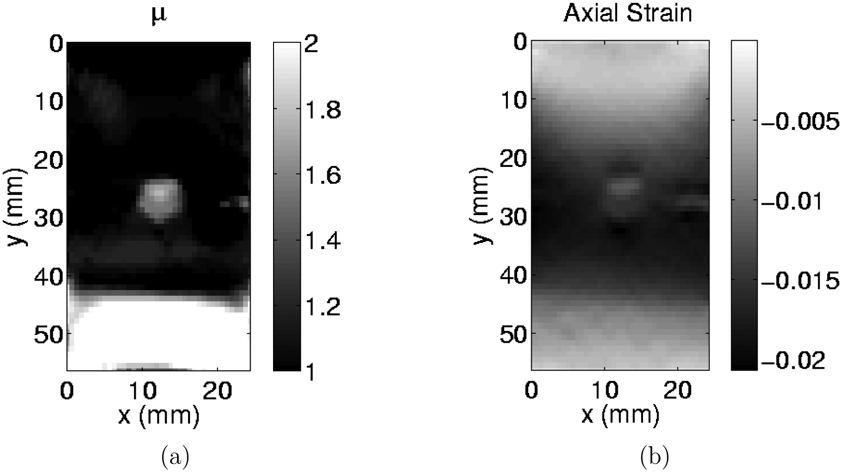
(a) slice of modulus reconstruction for a small inclusion with a 12% by mass gelatin concentration. (b) slice of the axial strain for this same inclusion. (Images are extracted from Tables 2 and 4)
Quantitatively, we may compare the reconstructed stiffness contrast to the calibration measurements of the separate samples, as reported in Table 1. This table shows that for the two higher concentrations, the reconstructed contrasts tend to be lower than the reference values. This apparent bias could be explicable by a number of reasons. For one, we use regularization in both our displacement estimation algorithm and in our modulus reconstruction methods. Regularization tends to bias reconstructed contrast downward; c.f. Figure 6(d), in which the line plot with simulated data shows a diminished inclusion contrast in the 3D reconstruction. For another, we compute the inclusion stiffness as the arithmetic mean of pixel values within half-maximum. This average is always lower, and typically significantly lower, than the peak value of the inclusion stiffness. Finally, the reference contrast values themselves may be in error as discussed below.
Figure 6.
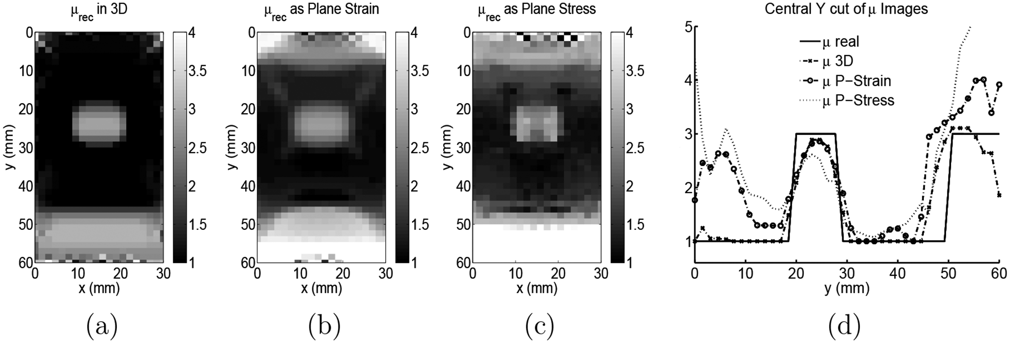
(a) Example slice of modulus reconstruction using 3D reconstruction and all 3 vector components. (b) 2D modulus reconstruction using the center slice of simulated 3D displacement data and a plane strain reconstruction. (c) 2D modulus reconstruction using the center slice of simulated 3D displacement data and a plane stress reconstruction. (d) Center axial line of all three modulus reconstructions in addition to the original modulus distribution used to create the displacements.
For the two lowest contrast inclusions the discrepancy between the reference contrast and the reconstructed contrast is likely due to error in the reference contrast. The independent mechanical tests suggest that the inclusions should be invisible, yet they are clearly seen in both strain and modulus images. Furthermore, a lack of contrast is at odds with the gelatin concentrations used in the background and the inclusion, approximately 8% and 10%, respectively. As we discuss in detail below, the variability of gelatin with temperature, in conjunction with the variability in the mechanical testing itself, is likely to be responsible for the lack of measurable contrast in the mechanical tests at the lowest contrast. The fact that the inclusions were resolved in the strain images and the reconstructed modulus images is highly suggestive that some contrast does exist between these gelatin concentrations.
The volume of the reconstructed inclusion relative to its actual volume shows significant relative variability, but no apparent bias. In nearly all cases it is within ±1/2 voxel side length in the linear dimensions of the sample. It seems to be most accurate for the medium sized inclusions and highest contrast. Certainly the volume of the reconstructed inclusion will depend on the somewhat arbitrary selection of the inclusion boundary which was chosen at the half maximum of the inclusion modulus value.
4.3. Three dimensional effects
Three-dimensional reconstructions represent an improvement over their two-dimensional counterparts not only because they reveal the 3D structure of the underlying material, but also because they incur no assumptions regarding the stress/strain-state. In 2D reconstructions a state of plane stress or plane strain must be assumed, even though the actual state may be very different from both these cases. This may lead to errors in reconstructions as we demonstrate in the following example.
Figure 6 shows a comparison between modulus images reconstructed from finite-element simulated 3D data. The generated data is designed to model a typical ultrasound tissue mimicking phantom (see Section 2.1) in size, geometry and modulus contrast (1 to 3 for background to inclusion and calibration layer). The boundary conditions applied to generate the data are made to approximate those of a typical experimental protocol and only that portion of the displacement field which falls directly below the surface at the acoustic window (i.e. the “imaged” volume) is considered for the inverse problem. In this example, white Gaussian noise is added to the resulting displacement field such the signal to noise ratios are approximately 20, 1800 and 20 for the lateral, axial and elevational displacements, respectively.
Figure 6(a) is the center slice of the reconstruction which utilizes all 3 components of the displacement field in the entire volume. Figure 6(b) and (c) are reconstructions done using the axial and lateral displacement components only of the central slice of the simulated data and a plane strain and plane stress approximation, respectively. Mixed boundary conditions were used on the lateral sides for all three reconstructions as described above. Figure 6(d) is a center line cut though the inclusion of all three reconstructions and the original modulus distribution used to create the simulated displacements.
5. Discussion
5.1. Displacement estimation
This paper introduces a method to measure the displacement from sets of ultrasound images of breast tissue or breast tissue mimicking materials at two different deformation states. The novel features of this method include the use of finite element interpolation, the use of global information for each nodal estimation and the systematic incorporation of prior knowledge to stabilize the estimated displacements. This is in contrast to typical feature tracking algorithms common in elastography, utilizing rigid block matching methods which tend to result in noisy displacement measurements. The finite element interpolation allows for distorted (strain compensated) elements and nonuniform meshes. The use of regularization improves the displacement estimates to some extent. Large values of the regularization parameter, however, can introduce unwanted artefacts in the displacement estimates, decreasing the accuracy of the algorithm. The incompressibility constraint also helps to decrease the noise in the solution, however, it is noted that this constraint may not be appropriate for all applications (i.e. tissue types). The size of the finite element mesh was chosen based on the upper limit of the matrix size that our hardware would allow. However, it is noted that when computational speed and size are minimal factors, this value should be chosen as the expected resolution of the displacement measurements calculated from the resolution and SNR of the ultrasound system (Walker & Trahey 1995, Weinstein & Weiss 1983, Weinstein & Weiss 1984).
As alluded to earlier, one of the drawbacks of this algorithm is the presence of local minima. The prevalence of these minima is due to the highly oscillatory nature of the RF US images. To avoid these, the displacement accuracy metric (, see equation (14)) was calculated for each element at each iteration. Experience has shown that metric values which are higher than 0.2 typically indicate regions which are stuck in local minima (a metric value of 0.2 would correspond to a peak normalized cross correlation value of approximately 0.9). Although several methods may be employed to avoid local minima, we chose to identify these regions with the norm measure and manually smooth these areas with surrounding areas which are not in local minima.
5.2. Modulus reconstruction
The inversion and reconstruction algorithm introduced in this paper provides a technique to infer underlying mechanical properties of tissue, given displacement measurements and an appropriate choice of model. This method utilizes a quasi-Newton method for optimization. The novel features of this algorithm include the use of total variation diminishing (TVD) regularization with piece-wise constant interpolation and the ability to reconstruct three dimensional structure.
The reference stiffness measurements exhibited a high degree of variability. This is thought to be due to a combination of limitations of the measurement protocol and inherent variability of gelatin properties. For example, despite efforts to limit slipping at the boundary during mechanical compression tests, it is possible that some visibly undetectable degree of slipping took place. If so, this presumably occurred to a different extent in each experiment. Furthermore, gelatin stiffness itself is known to have a high variability depending on the length of time between setting and testing, due to water loss, as well as the temperature at which it was tested (Hall et al. 1996). To reduce these effects, both the imaging phantoms and the calibration samples were tested within 24 hours of their construction. They were tested immediately following their removal from refrigeration and kept sealed during refrigeration to limit water loss. The difference in size between the imaging phantoms and the calibration samples may also have contributed to the error. For instance, the small size of the calibration samples could result in a higher temperature variation across the samples. In addition, the larger length of the imaging experiment and the relatively large size of the phantoms could result, at least to some degree, to a larger temperature variation within the phantom volume, as well as some possible water loss within the phantom, during testing. The effect of the latter would be to stiffen the phantom non-uniformly, beginning with the exposed surfaces of the phantom (not the reconstructed surface). The temperature variation, resulting from both the length of the exam and the US image heating, would effectively soften the phantom non-uniformly. Although it is assumed in this work that these effects are minimal, they cannot be ignored. We believe that a combination of all these effects are responsible for the apparent inability to measure the contrast in the reference samples in the lowest contrast inclusions. Even considering all these possible sources of error, it was somewhat reassuring that the reconstructed modulus contrast was within about 35% of the reference values for all cases considered.
Choosing the value of the regularization constant remains a challenge. The “strength” of the regularization term in the functional is affected not only by the magnitude of the parameter, but also the size and contrast of the underlying modulus distribution. Thus, regularization will tend to play a larger role in modulus distributions with higher contrasts and larger sizes. We also note that the presence of the surrounding artefacts is more obvious for lower inclusion contrasts than larger. It is possible that increasing the regularization in these cases, to try and further minimize the artefacts, may cause the low contrast inclusion to be lost. To a certain extent, an optimal choice of regularization constant can be selected using a priori knowledge of the target contrast of inclusions. Such results present an unrealistic impression of the effectiveness of inversion in practice, however, where such knowledge would be unavailable. In this work we tried to avoid such bias by selecting the regularization parameter through simulated experiments. We then used precisely the same regularization parameter for all subsequent inversions. In retrospect, we feel it likely that the reconstructions above are over-regularized, and therefore biased toward low contrasts. An opportunity exists in the field to develop an adaptive automated regularization method for each construction, to simultaneously control noise and preserve contrast.
Our study indicates that the algorithm used for modulus reconstruction is sensitive to the choice of boundary conditions. This dependence needs to be explored in future research. It also appears to indicate that traction boundary conditions lead to better reconstructions. This implies that devices that are able to measure surface traction in addition to making ultrasound measurements will be very useful in elasticity imaging. Another approach to mitigating the effect of boundary conditions might be to use more than one deformation field in evaluating the shear modulus. How much this would help is yet to be determined.
The bottom layer was remarkably difficult to resolve. This is due, in part, to the role of boundary conditions in computing the predicted displacement field and to the uniqueness issues tied closely to those boundary conditions. In this inverse problem, the use of Dirichlet (e.g. displacement) boundary conditions decreases the sensitivity of the inversion near these boundaries (see Table 3). That is, in areas where the boundaries are all Dirichlet, the predicted displacements are fixed and therefore independent of the estimate of . Thus in equation (9) the derivative of with respect to in these regions is practically zero. A direct consequence of this is that in these regions the value of tends to remain “frozen” at its initial value and the modulus estimate does not improve. Since the bottom layer is adjacent to a boundary, reconstructions with all displacement boundary conditions resulted in little to no recovery of this layer. On the other hand, using traction boundary conditions adds information to the reconstruction additional to the measured displacement field (see Table 2). It was found during simulations that with the sides of the reconstructed volume (i.e. the and boundary surfaces) assumed to have zero normal traction ( on and ) and the remaining boundary conditions Dirichlet conditions, the bottom layer and the field as a whole resulted in the most accurate modulus distributions. Although this choice of boundary conditions are inexact we expect, based on our phantom geometry and experimental setup, that they are a reasonable approximation. Indeed, the information they add evidently improves the reconstruction significantly. At the same time, however, the approximate nature of these boundary conditions did introduce some artefacts into the images, particularly at the edges where the calibration layer lies. This, we believe, led to the high variability observed in the accuracy of the reconstructed bottom layer (see the figures in Table 2).
It is clear from Figure 6 that the three dimensional modulus reconstruction results in a better representation of underlying modulus. In this case, the plane strain reconstruction is better than the plane stress, but neither is as good as the 3D reconstruction. In addition, it’s worth noting that while plane strain seems better in this example, other examples might be created where plane stress gives a more accurate reconstruction than does plane strain.
The adjoint method for gradient evaluation is crucial for the practical solution of this problem. The modulus reconstructions were performed on a 40×60×40 element mesh, which leads to 96×103 ≈ 105 optimization variables. Any scheme whose major computational cost scales poorly, even linearly, with the number of optimization variables would have been impractical in solving this problem. The adjoint method gives us the gradient with just two forward solves, independent of the number of optimization variables. This technique makes the solution of this problem feasible.
It has been well documented that the inverse problem considered here has a non-unique solution (Barbone & Gokhale 2004, Barbone & Bamber 2002, Richards 2007). That is, several distinct modulus distributions are all equally consistent with the measured displacement field. We note, however, that our reconstructions are based on more information than just the measured displacement field. In particular, information is added in three specific places: the assumed boundary conditions, the optimization formulation, and the regularization function.
The sides of the reconstructed volume (i.e. those surfaces parallel to the axial direction) are assumed to have zero normal traction. That is, we assume there is no confining pressure around the sides of the phantom. This is roughly consistent with the physical experiment. This also helps with the reconstruction as specifying traction boundary conditions substantially reduces the dimension of the solution space, and thereby alleviates the non-uniqueness of the problem (Barbone & Bamber 2002, Richards 2007).
The modulus is reconstructed relative to the background value, which we arbitrarily set at unity. We set this as the lower limit for the modulus distribution, and initialize our iterations there. Thus, we bias the search to seek stiff inclusions in a compliant homogeneous background. Finally, the TVD regularization used here biases towards piece-wise constant modulus distributions. The results indicate that this seems to be a relatively weak effect in our reconstructions. These three sources of information inform our reconstructions. Significantly altering any one of them could significantly change the reconstruction, even with exactly the same input displacement data. Thus the reconstructions represent a synthesis of these different sources of information, above and beyond what is contained in the measured displacement field.
6. Conclusions
We have developed and implemented an algorithm for the accurate measurement of a three dimensional displacement field from ultrasound images of deforming tissue. The novel features of this algorithm include the use of finite element discretization, the inclusion of a priori knowledge of the material’s incompressibility and the use of regularization. We have also developed an efficient formulation to solve the three dimensional inverse elasticity problem using a full three dimensional displacement field measurement. The novel features of this approach include the use of a gradient based algorithm and the efficient computation of the gradient using the adjoint equations. By using these techniques we have successfully imaged and reconstructed phantom inclusions as small as 5.0 mm and with contrasts approaching unity. The development of an accurate, quantitative method by which to measure and image the mechanical properties of materials, such as is outlined in this paper, is a significant step forward in the field of elasticity imaging. It offers a noninvasive method to interrogate mechanical properties in vivo for the purposes of diagnosis and monitoring.
Future work will include further investigation into the uniqueness of the three dimensional inverse elasticity problem and the relationship between the imposed boundary conditions and the modulus reconstructions. In addition, an initial clinical investigation of three dimensional breast ultrasound elasticity imaging is currently underway.
Figure 1.
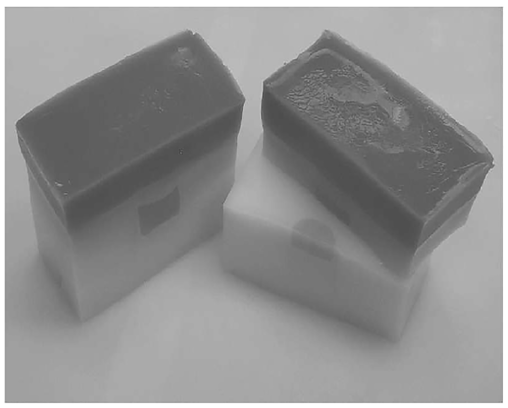
Ultrasound Elasticity Gelatin Phantom
Figure 4.
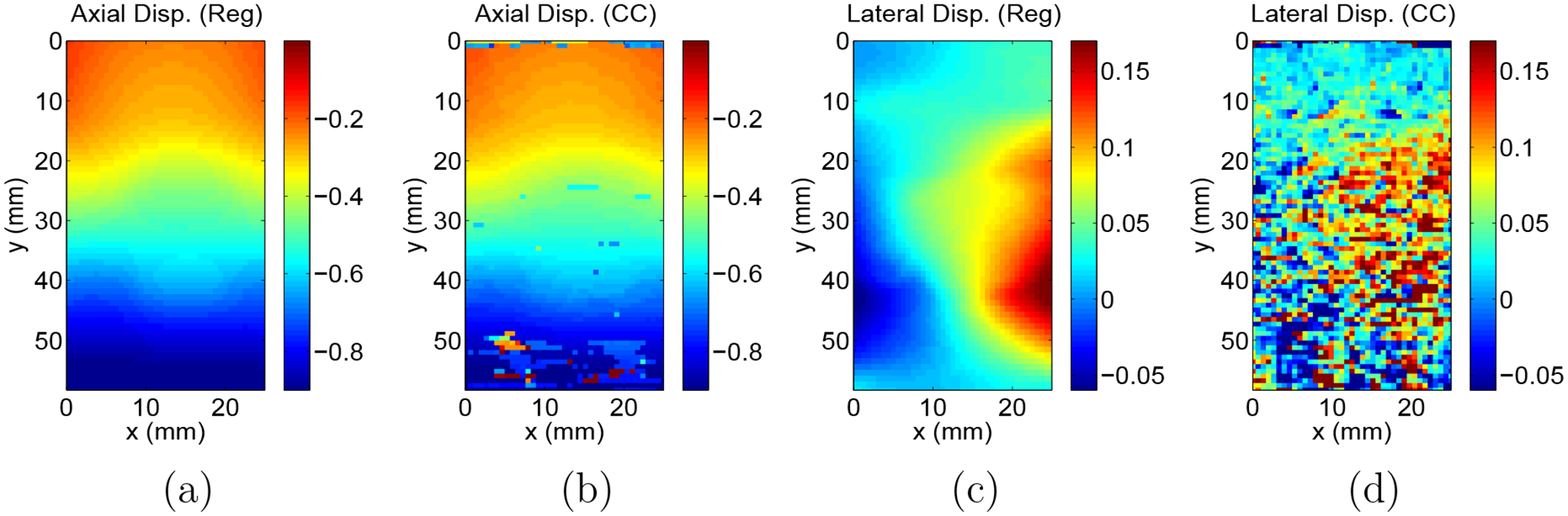
Example slice of axial displacements measured using the image registration technique (a) and using a cross correlation method (b). Corresponding slice of lateral displacements measured using the image registration technique (c) and using a cross correlation method (d))
Acknowledgments
The authors would like to thank the Biomedical Microdevices and Microenvironments Laboratory and the Physical Acoustics Laboratory at Boston University for their generous lending of research space and equipment. This work benefitted greatly from discussions with Dr. Jonathan M Rubin at the University of Michigan. This work was supported in part by NSF Award No. EEC-9986821, DOD Breast Cancer Research Program Award No. W81XWh-04-1-0763, and NIH Grants RO1CA91713 and R21CA109440.
Appendix A. Parameter Value Evaluation
In this section, we describe a series of experiments for each algorithm (displacement measurement and inversion), which are designed to determine the appropriate choice of the algorithms’ parameters. Once these parameters are determined they are used without any modifications in the actual reconstruction experiments. For each algorithm, artificial input is created from a known solution so that for the given input we have a reference or “true” value to compare to the algorithm output. For example, in the case of the displacement estimation algorithm, we acquired a single 3D US RF image using the phantoms and experimental setup described in Section 2. Then a second, pre-deformation, image is created artificially by defining the spatial locations of the first image’s pixels and interpolating that image at as is shown in equation (1). In these experiments, is chosen to correspond to an unconfined compression test with slip boundaries of a homogeneous block of incompressible linear elastic material at a strain level of 4%. Thus the displacement field is linear in each direction and volume conserving. The second image was interpolated using MATLAB’s Interp3 function and cubic interpolation (The MathWorks, Inc., 3 Apple Hill Drive Natick, MA 01760). Then these images were input to the displacement estimation algorithm, with various values of the regularization parameter and the incompressibility parameter , which then resulted in a corresponding measured displacement field .
The error in the resulting measurement was then quantified as the Euclidean norm of the difference in the measurement and reference displacement field ) for each displacement vector component (i). Several values of were tested within a range spanning the approximate expected value and for each value of several values of , again spanning the relevant range, were also tested. The experiment was repeated for 5 sets of images, where the initial, experimentally created image, was taken of different phantoms or different regions within the same phantom to ensure that the resulting image sets were uncorrelated. The experiment was also repeated for various finite element mesh sizes to determine the accuracy of the measurement as a function of the resolution.
The values of the parameters which consistently minimized the total displacement measurement error () were those used in the displacement estimation of all the subsequent phantom experiments in this paper. In these experiments there was no significant change in accuracy for the different mesh sizes and thus the mesh size used in this paper represented the upper limit that our computational resources would allow. It should be noted that previous experiments have shown that the electronic noise of the imaging system is not the dominant source of error affecting the accuracy of this algorithm and thus electronic noise was neglected in this parameter evaluation study (Richards 2007).
A similar set of experiments was performed for the reconstruction algorithm. Here a modulus distribution is created to model a typical ultrasound tissue-mimicking phantom in size and geometry, including an inclusion and bottom layer. The size of the inclusion and the modulus contrast of the inclusion and bottom layer were chosen to be approximately equivalent to the large sized inclusion and the highest contrast of those tested in the actual phantom experiments. An artificial displacement field was then created, using this modulus distribution and a forward finite element analysis. This displacement field was created on a finite element mesh which was spatially refined by 1.25 times that of the subsequent reconstruction meshes to ensure that the forward problem was well resolved. The boundary conditions applied to this modulus distribution were selected to approximate those of a typical experimental protocol. Then only that portion of the displacement field, which would correspond to the imaged volume experimentally, was then considered for this parameter evaluation.
The relevant parameters for the reconstruction algorithm are the Poisson’s ratio , the boundary conditions used in the reconstruction, the optimal weighting of the displacement estimates and the regularization parameter . To determine the choice of the Poisson’s ratio for the reconstructions, various displacement fields were created using several different values of the Poisson’s ratio of nearly incompressible materials in the forward problem described above. These displacement fields were then input to the reconstruction algorithm to create a predicted modulus field . For each choice of Poisson’s ratio in the forward problem, several reconstructions were performed assuming a similar set of Poisson’s ratios in the inversion algorithm. Again, the error in the measurement is quantified by the Euclidean norm of the predicted and reference values . The results of these simulations suggested that the accuracy of the modulus reconstruction has little dependence on the choice of Poisson’s ratio used in the reconstruction or the “true” material Poisson’s ratio when both were greater than 0.495 and less than 0.5. The boundary conditions for this study’s reconstructions were prescribed displacements. was set to the second order identity tensor and the regularization parameter was set to zero.
Contrary to Poisson’s ratio, the choice of boundary conditions can have a large impact on the reconstruction accuracy. For the purposes of this paper, reconstructions with two types of boundary conditions were investigated using the same process of forward modeling and subsequent reconstruction. The first type of boundary conditions investigated all prescribed displacement, or Dirichlet, boundary conditions. The second type of boundary conditions investigated allowed a portion of the boundary to be traction free in the direction of the surface normal. In the latter case, the sides of the reconstructed volume (i.e. those surfaces parallel to the axial direction) were assumed to have zero normal traction and the remaining boundary conditions were Dirichlet conditions. It was found that the “zero normal traction” yielded the highest accuracy for our modulus geometry and thus these boundary conditions were used in all of the gel phantom reconstructions presented here. However, for comparison purposes, reconstructions using all Dirichlet boundary conditions for all the phantoms tested are provided in Table 3. There was no noise introduced in this study and as such was again set to the identity matrix and the regularization parameter was set to zero.
The weighting matrix was determined from estimates of error in the displacement components. In particular, the diagonal components and and the off diagonal components were set to 0. These values were based on our estimate that the axial (y) displacements are a factor of 10 times more accurate than the lateral (x) and elevational (z) displacements.
To determine the appropriate choice of the reconstruction regularization parameter , a series of reconstructions were performed on artificial displacement fields, created as described above. White Gaussian noise was added to these displacement estimates, prior to reconstruction, with error magnitudes equal to those realized in practice (calculated in the displacement estimation study). A series of reconstructions are performed with various values of the regularization parameter producing a corresponding predicted modulus distribution. The accuracy was again monitored by calculating the Euclidian norm and the value of the regularization parameter which minimized this difference was used for all the subsequent modulus reconstructions in this paper.
It is important to note that, although the parameter evaluations of this section were determined from studies of only one possible realization of the displacement field and one possible realization of the actual modulus distribution , the optimal values of the parameters found here were held constant for all the measurements and reconstructions done in the actual phantom experiments.
References
- Bamber JC, Barbone PE, Bush NL, Cosgrove DO, Doyley MM, Fueschel FG, Meaney PM, Miller NR, Shiina T & Tranquart F 2002. The Insitute of Electronics, Information and Communication Engineers Transactions on Information and Systems E85-D, 5–15. [Google Scholar]
- Barbone PE & Bamber JC 2002. Physics in Medicine and Biology 47, 2147–2164. [DOI] [PubMed] [Google Scholar]
- Barbone PE & Gokhale NH 2004. Inverse Problems 20, 283–296. [Google Scholar]
- Burnside ES, Hall TJ, Sommer AM, Hesley GK, Sisney GA, Svensson WE & Hangiandreou NJ 2007. Radiology 245, 401–410. [DOI] [PubMed] [Google Scholar]
- Doyley MM, Meaney PM & Bamber JC 2000. Physics in Medicine and Biology 45. [DOI] [PubMed] [Google Scholar]
- Doyley M, Srinivasan S, Pendergrass S, Wu Z & Ophir J 2005. Ultrasound in Medicine and Biology 31, 787–802. [DOI] [PubMed] [Google Scholar]
- Garra BS, Céspedes EI, Ophir J, Spratt SR, Zuurbier RA, Magnant CM & Pennanen MF 1997. Radiology 202, 79–86. [DOI] [PubMed] [Google Scholar]
- Giuseppetti GM, an BD Cioccio AM & Baldassarre S 2005. Radiologia Medica 110, 69–76. [PubMed] [Google Scholar]
- Gokhale NH, Richards MS, Oberai AA, Barbone PE & Doyley MM 2004. IEEE International Symposium on Biomedical Imaging: Macro to Nano 1, 543–546. [Google Scholar]
- Hall TJ, Bilgen M, Insana MF & Chaturvedi P 1996. Proceedings of the IEEE Ultrasonics Symposium 2, 1193–1196. [Google Scholar]
- Hall TJ, Zhu Y & Spalding CS 2003. Ultrasound in Medicine and Biology 29, 427–435. [DOI] [PubMed] [Google Scholar]
- Hughes TJR 1999. The Finite Element Method Dover Publications. [Google Scholar]
- Itoh A, Ueno E, Tohno E, Kamma H, Takahashi H, Shiina T, Yamakawa M & Matsumaura T 2006. Radiology 239, 341–350. [DOI] [PubMed] [Google Scholar]
- Kallel F & Bertrand M 1996. IEEE Transactions on Medical Imaging 15, 229–313. [DOI] [PubMed] [Google Scholar]
- Krueger M, Pesavento A, Ermert H, Hiltawsky K, Heuser L, Rosenthal H & Jensen A 1998. Ultrasonics Symposium, 1998. Proceedings., 1998 IEEE 2, 1757–1760 vol.2. [Google Scholar]
- Lindop JE, Treece GM, Gee AH & Prage RW 2006. Ultrasound in Medicine and Biology 37 (4), 529–545. [DOI] [PubMed] [Google Scholar]
- Lorenz A, Pesavento A, Pesavento M & Ermert H 1999. Ultrasonics Symposium, 1999. Proceedings. 1999 IEEE 2, 1657–1660 vol. 2. [Google Scholar]
- Nocedal J 1980. Mathematics of Computation 35, 773–782. [Google Scholar]
- Oberai AA, Gokhale NH, Doyley MM & Bamber JC 2004. Physics in Medicine and Biology 49, 2955–2974. [DOI] [PubMed] [Google Scholar]
- Oberai AA, Gokhale NH & Feijóo GR 2003. Inverse Problems 19, 297–313. [Google Scholar]
- Ophir J, Céspedes I, Ponnekanti H, Yazdi Y & Li X 1991. Ultrasonic Imaging 13, 111–134. [DOI] [PubMed] [Google Scholar]
- Raghavan KR & Yagle AE 1994. IEEE Transactions on Nuclear Science 41, 1639–1648. [Google Scholar]
- Regner DM, Hesley GK, Hangiandreou NJ, Morton MJ, Nordland MR,, Meixner DD, Hall TJ, Farrell MA, Mandrekat JN, Harmsen S & Charboneau JW 2006. Radiology 238, 425–437. [DOI] [PMC free article] [PubMed] [Google Scholar]
- Richards M 2007. Qunatitative Three Dimensional Elasticity Imaging PhD thesis Boston University. [Google Scholar]
- Schenk O & Gartner K 2004. Journal of Future Generation Computer Systems 20, 475–487. [Google Scholar]
- Schenk O & Gartner K 2006. Electronic Transaction On Numerical Analysis 23, 158–179. [Google Scholar]
- Skovoroda AR, Emelianov SY & O’Donnell M 1995. IEEE Transactions on Ultrasonics, Ferroelectronics, and Frequency Control 42, 747–765. [Google Scholar]
- Steele DD, Chenevert TL, Skovoroda AR & Emelianov AY 2000. Physics in Medicine and Biology 45, 1633–1648. [DOI] [PubMed] [Google Scholar]
- Sumi C 2006. IEEE Transactions on Ultrasonics, Ferroelectrics, and Frequency Control 53 (12), 2416–2434. [DOI] [PubMed] [Google Scholar]
- Thomas A, Fischer T, Frey H, Ohlinger R, Grunwald S, Blohmer J, Winzer K, Weber S, Kristiansen G, Ebert B & Kummel S 2006. Ultrasound in Obstetrics and Gynecology 28, 335–340. [DOI] [PubMed] [Google Scholar]
- Treece GM, Lindop JE, Gee AH & Prager RW 2008. Ultrasound in Medicine 8 Biology 34(3), 463–474. [DOI] [PubMed] [Google Scholar]
- Vogel CR 2002. Computational Methods for Inverse Problems SIAM. [Google Scholar]
- Walker WF & Trahey GE 1995. IEEE Transactions on Ultrasonics, Ferroelectrics, and Frequency Control 42, 301–308. [DOI] [PubMed] [Google Scholar]
- Weinstein E & Weiss A 1983. IEEE Transactions on Acoustic, Speech and Signal Processing 31, 472–485. [Google Scholar]
- Weinstein E & Weiss A 1984. IEEE Transactions on Acoustic, Speech and Signal Processing 31, 1064–1078. [Google Scholar]
- Weismann C 2005. Springer Tokyo chapter Recent Advances in Multidimensional 3D/4D Breast Imaging, pp. 146–150. [Google Scholar]
- Zhi H, Ou B, Luo BM, Feng X, Wen YL & Yang HY 2007. Journal of Ultrasound in Medicine 26, 807–815. [DOI] [PubMed] [Google Scholar]