Dhaka: variational autoencoder for unmasking tumor heterogeneity from single cell genomic data

Abstract

Motivation

Intra-tumor heterogeneity is one of the key confounding factors in deciphering tumor evolution. Malignant cells exhibit variations in their gene expression, copy numbers and mutation even when originating from a single progenitor cell. Single cell sequencing of tumor cells has recently emerged as a viable option for unmasking the underlying tumor heterogeneity. However, extracting features from single cell genomic data in order to infer their evolutionary trajectory remains computationally challenging due to the extremely noisy and sparse nature of the data.

Results

Here we describe ‘Dhaka’, a variational autoencoder method which transforms single cell genomic data to a reduced dimension feature space that is more efficient in differentiating between (hidden) tumor subpopulations. Our method is general and can be applied to several different types of genomic data including copy number variation from scDNA-Seq and gene expression from scRNA-Seq experiments. We tested the method on synthetic and six single cell cancer datasets where the number of cells ranges from 250 to 6000 for each sample. Analysis of the resulting feature space revealed subpopulations of cells and their marker genes. The features are also able to infer the lineage and/or differentiation trajectory between cells greatly improving upon prior methods suggested for feature extraction and dimensionality reduction of such data.

Availability and implementation

All the datasets used in the paper are publicly available and developed software package and supporting info is available on Github https://github.com/MicrosoftGenomics/Dhaka.

Supplementary information

Supplementary data are available at Bioinformatics online.

1 Introduction

Tumor cells are often very heterogeneous. Typical cancer progression consists of a prolonged clinically latent period during which several new mutations arise leading to changes in gene expression and DNA copy number for several genes (Andor et al., 2016; de Bruin et al., 2014; Min et al., 2015). As a result of such genomic variability, we often see multiple subpopulations of cells within a single tumor.

The goal of effective cancer treatment is to treat all malignant cells without harming the originating host tissue. Clinical approaches should thus take into account the underlying evolutionary structure in order to identify treatments that can specifically target malignant cells while not affecting their normal cell of origin. It is also important to determine if the ancestral tumor clones eventually disappear (chain like evolution) or if several genotypically different clones of cells evolved in parallel (branched evolution) (de Bruin et al., 2014). Tumors resulting from these two evolutionary trajectories respond differently and ignoring the evolutionary process when determining treatment can lead to therapy resistance and possible cancer recurrence. Thus, characterization of the hidden subpopulations and their underlying evolutionary structure is an important issue for both the biological understanding and clinical treatment of cancer. Prior studies have mainly relied on bulk sequencing to investigate tumor evolution (Navin and Hicks, 2010; Russnes et al., 2011). In such experiments thousands of cells are sequenced together, which averages out the genomic characteristics of the individual cells making it hard to infer these subpopulations. More recently, single cell sequencing has emerged as a useful tool to study such cellular heterogeneity (Giustacchini et al., 2017; Tirosh et al., 2016b; Venteicher et al., 2017; Zahn et al., 2017).

While single cell data are clearly much more appropriate for addressing tumor heterogeneity and evolution, it also raises new computational and experimental challenges. Due to technical challenges (e.g. the low quantity of genetic material and the coverage for each of the cells sequenced) the resulting data are often very noisy and sparse with many dropout events (Gawad et al., 2016; Zong et al., 2012). These issues affect both scRNA-Seq and scDNA-Seq experiments which are used for copy number and mutation estimation. Given these issues, it remains challenging to identify meaningful features that can accurately characterize the single cells in terms of their clonal identity and differentiation state. To address this, several methods have been proposed to transform the observed gene expression or copy number profiles in order to generate features that are more robust for downstream analysis. However, as we show below, many of the feature transformation techniques that are usually applied to genomic data fail to identify the subpopulations and their trajectories. For example, while t-distributed Stochastic Neighbor Embedding (t-SNE) (Maaten and Hinton, 2008) and diffusion maps (Roweis and Saul, 2000) are very successful in segregating cells between different tumor samples, they are less successful when trying to characterize the evolutional trajectories of a single tumor. Recently, several unsupervised feature transformation techniques were proposed for analysis of single-cell RNA-seq data (DeTomaso and Yosef, 2016; Li et al., 2017; Pierson and Yau, 2015; van Dijk et al., 2017; Wang et al., 2017). Among these tools, ZIFA (Pierson and Yau, 2015) explicitly models the drop out event in single cell RNA-seq data to improve the reduced dimension representation whereas SIMLR (Wang et al., 2017) developed a new similarity learning framework that can be used in conjunction with t-SNE to reduce dimension of the data. MAGIC (van Dijk et al., 2017) is another dimensionality reduction method that uses data diffusion to denoise the cell count matrix and fill in missing transcripts. In addition to dimensionality reduction methods, several single cell clustering algorithms have been proposed as well (Fan et al., 2016; Xu and Su, 2015). SNN-cliq (Xu and Su, 2015) constructs a shared k-nearest neighbor graph across all cells and then finds maximal cliques and PAGODA relies on prior set of annotated genes to find transcriptomal heterogeneity. All these methods can successfully distinguish between different groups of cells in a dataset. However, such methods are not designed for determining the relationship between the detected clusters which is the focus of tumor evolutionary analysis. In addition, most current single cell clustering methods are focused on only one type of genomic data (e.g. scRNA-Seq) and do not work well for multiple types of such data.

Another direction that has been investigated for reducing the dimensionality of scRNA-Seq data is the use of neural networks (NN) (Gupta et al., 2015; Lin et al., 2017). In Lin et al. (2017), the authors used prior biological knowledge including protein–protein and protein–DNA interaction to learn the architecture of a NN and to subsequently project the data to a lower dimensional feature space. Unlike these prior approaches, which were supervised, we are using NN in a completely unsupervised manner and so do not require labeled data as prior methods have. Specifically, in our software ‘Dhaka’ we have used a variational autoencoder (VAE) based approach that combines Bayesian inference with unsupervised deep learning, to learn a probabilistic encoding of the input data. Another VAE based single cell method was also proposed very recently for RNA-seq data, scVI (Lopez et al., 2017). The method uses explicit modeling of technical effects in RNA-seq data generation (batch effect, technical drop outs) and then uses t-SNE for visualization (Lopez et al., 2017). In contrast, here we aim for a generalized dimensionality reduction method across different platforms (RNA-seq, copy number). Specifically, in this paper we have analyzed four scRNA-Seq and two scDNA-Seq datasets. We used the VAE to project the expression and copy number profiles of tumor populations and were able to capture clonal evolution of tumor samples even for noisy sparse datasets with very low coverage. We also compare the performance of Dhaka with four generalized dimensionality reduction methods, principal component analysis (PCA) (Jolliffe, 1986), t-SNE (Maaten and Hinton, 2008), non-negative matrix factorization (NMF) (Lee and Seung, 2001), regular autoencoders (Hinton and Salakhutdinov, 2006) and four specialized single cell dimensionality method, ZIFA (Pierson and Yau, 2015), SIMLR (Wang et al., 2017), MAGIC (van Dijk et al., 2017) and scVI (Lopez et al., 2017). While it is difficult to include all the existing methods for single cell visualization for comparative performance analysis, we have tried to compare to methods that are methodologically very different from each other and have been shown to perform well on multiple single cell datasets. Dhaka shows significant improvement over the prior methods thus corroborating the effectiveness of our method in extracting important biological and clinical information from cancer samples.

2 Materials and methods

2.1 VAE

We used a VAE to analyze single cell genomic data. For this, we adapted a VAE initially proposed by Kingma and Welling (2013). Autoencoders are multilayered perceptron NN that sequentially deconstruct data (x) into latent representation (z) and then use these representations to reconstruct outputs that are similar (in some metric space) to the inputs. The main advantage of this approach is that the model learns the best features and input combinations in a completely unsupervised manner. In VAEs unsupervised deep learning is combined with Bayesian inference. Instead of learning an unconstrained representation of the data we impose a regularization constraint. We assume that the latent representation is coming from a probability distribution, in this case a multivariate Gaussian ($N({\mu }_z,{\sigma }_z)$). The intuition behind such representation for single cell data is that the heterogeneous cells are actually the result of some underlying biological process leading to the observed expression and copy number data. These processes are modeled here as distribution over latent space, each having their distinct means and variances. Hence the autoencoder actually encodes not only the means (μ_z) but also the variances (σ_z) of the Gaussian distributions. The latent representation (z) is then sampled from the learned posterior distribution $q_{\varphi }(z|x)\sim N({\mu }_z,{\sigma }_{z}I)$. Here $\varphi$ are the parameters of the encoder network (such as biases and weights). The sampled latent representation is then passed through a similar decoder network to reconstruct the input $\overline{x}\sim p_{\theta }(x|z)$, where θ are the parameters of the decoder network. Although the model is trained to minimize the error between the inputs and the reconstructed outputs, we are actually interested in the latent representation z of the data since it represents the key information needed to accurately reconstruct the inputs.

2.2 Model structure

Figure 1 presents the structure of the autoencoder used in this paper. The input layer consists of nodes equal to the number of genes we are analyzing for each cell. The input to the Dhaka package is log2 transformed TPM counts. We have used Rectified Linear unit (ReLu) activation function in all the layers except the final layer of getting the reconstructed output. We used sigmoid activation function in the final layer (We have option of using ReLU activation in the final layer as well. Performance with ReLU activation function can be found in the Appendix.). We have used three intermediate layers with 1024, 512 and 256 nodes and a 3D latent layer. The latent layer has three nodes for mean (μ_z) and three nodes for variance (σ_z), which generate the 3D latent variable z. The size of the latent dimension (i.e. the representation we extract from the model) is a parameter of the model. As we show in Section 3, for the data analyzed in this paper three latent variables are enough to obtain accurate separation of cell states for both the expression and copy number datasets. Increasing this number did not improve the results and so all figures and subsequent analysis are based on this number. However, the method is general and if needed can use more or less nodes in the latent layer.

Fig. 1.

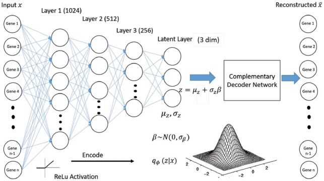
Structure of the VAE used in Dhaka. We have three intermediate dense layers of 1024, 512 and 256 nodes between the input and latent layer. All the layers in the encoder and decoder network use ReLu activation except the output layer (sigmoid activation). The latent layer has three nodes each for encoding mean and variances of the Gaussian distribution. The input of the decoder network, the latent representation z is then sampled from that distribution using the reparameterization trick (Kingma and Welling, 2013)

All datasets we analyzed had more than 5 K genes and the reported structure with at least 1024 nodes in the first intermediate layer (Fig. 1) was sufficient for them. We used three intermediate layers to gradually compress the encoding to a 3D feature space. We have also compared three different structures of autoencoders: (i) the proposed three intermediate layers, (ii) one intermediate layer and (iii) five intermediate layers in the Section 3.

2.3 Learning

To learn the parameters of the autoencoder, $\varphi$ and θ, we need to maximize $\log (p(x|\varphi ,\theta ))$, the log likelihood of the data points x, given the model parameters. The marginal likelihood $\log (p(x))$ is the sum of a variational lower bound (Kingma and Welling, 2013) and the Kullback–Leibler (Joyce, 2011) divergence between the approximate and true posteriors.

$$\log (p(x))=L(\varphi ,\theta ;x)+D_{\mathit{KL}}(q_{\varphi }(z|x)\left|\right|p_{\theta }(z|x)).$$

The likelihood L can be decomposed as following:

$$L(\varphi ,\theta ;x)=E_{z\sim q_{\varphi }(z|x)}[\log (p_{\theta }(x|z))]-D_{\mathit{KL}}(q_{\varphi }(z|x)||p_{\theta }(z)).$$

The first term can be viewed as the typical reconstruction loss intrinsic to all autoencoders, the second term can be viewed as the penalty for forcing the encoded representation to follow the Gaussian prior (the regularization part). We then use ‘RMSprop’, which relies on a variant of stochastic minibatch gradient descent, to minimize—L. In ‘RMSprop’, the learning rate weight is divided by the running average of the magnitudes of recent gradients for that weight leading to better convergence (Tieleman and Hinton, 2012). Detailed derivation of the loss computation can be found in Kingma and Welling (2013). To demonstrate the robustness of the training, we have shown the loss function plot from 50 independent trials on the Oligodendroglioma dataset (Supplementary Fig. S2). The low standard error (SE) in the plot corroborates the robustness of training in Dhaka.

An issue in learning VAE with standard gradient descent is that gradient descent requires the model to be differentiable, however the presence of stochastic sampling layer in VAE makes the model undifferentiable. To enable the use of gradient descent in our model, we use the reparameterization trick introduced in Kingma and Welling (2013). We introduce a new random variable β. Instead of sampling z directly from the $N({\mu }_z,{\sigma }_{z}I)$, we set

$$z={\mu }_z+{\sigma }_z*\beta .$$

Where β is the Gaussian noise, $\beta \sim N(0,{\sigma }_{\beta })$. Using β we do not need to sample from the latent layer and so the model is differentiable and gradient descent can be used to learn model parameters (LeCun et al., 2015). ${\sigma }_{\beta }$ is the standard deviation of the Gaussian noise and is an input parameter of the model.

3 Results

3.1 Simulated dataset

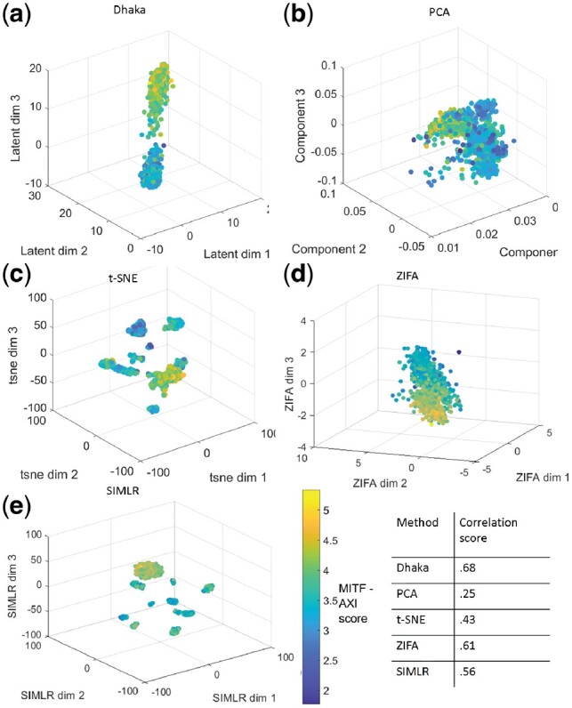
We first performed simulation analysis to compare the Dhaka method with prior dimensionality reduction methods that have been extensively used for scRNA-Seq data: t-SNE (Maaten and Hinton, 2008), PCA (Jolliffe, 1986), ZIFA (Pierson and Yau, 2015), SIMLR (Wang et al., 2017), NMF (Lee and Seung, 2001), regular autoencoder (Hinton and Salakhutdinov, 2006), MAGIC (van Dijk et al., 2017) and scVI (Lopez et al., 2017). Due to space constraint, we present the comparison with the first four methods here and the last four in the Appendix (Supplementary Fig. S5).We generated a simulated dataset with 3 K genes and 500 cells. In the simulated dataset, cells are generated from five different clusters with 100 cells each. There are a total of 3000 genes in the dataset. All the 3000 genes contain variable amount of noise, among which 500 genes have cluster specific expression to some extent and the remaining 2500 genes does not have any cluster specific expression, i.e. completely noisy. Detailed description of the simulated data generation can be found in Appendix 1.2.

We have used a Gaussian Mixture Model to cluster the reduced dimension data obtained from Dhaka and other competing methods and Bayesian information criterion (BIC) to select the number of clusters. We next compute the Adjusted Rand Index (ARI) metric to determine the quality of resulting clustering for each dimensionality reduction method. Figure 2 shows the result of Dhaka, PCA, t-SNE, ZIFA and SIMLR projection for the simulated data. As can be seen, the Dhaka autoencoder has the highest ARI score of 0.73. The closest is SIMLR (ARI: 0.70) and the ZIFA (ARI: 0.58). Although the Dhaka autoencoder identifies four clusters compared to SIMLR identifying 5, the cluster labels are better preserved in Dhaka leading to the higher ARI score. Among the comparing methods presented in the Appendix (Supplementary Fig. S5) only the regular Autoencoder has a high ARI score 0.72, with four identified clusters. The other methods (NMF, MAGIC and scVI) have score below 0.2. Implementation details of the competing methods can be found in Appendix 1.6. The VAE in Dhaka is optimized with no guaranteed global convergence. Hence we will see slightly different outputs with each run of the algorithm. We analyzed the robustness of the method to random initializations on the simulated dataset. With 10 random initializations we observed mean ARI of 0.73 with of 0.01. This relatively low SE corroborates the robustness of the proposed method.

Fig. 2.

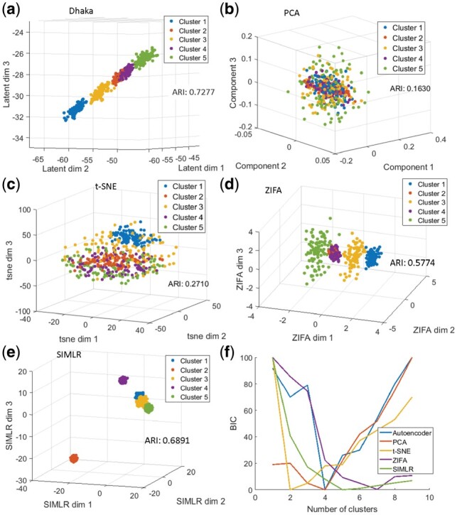
Comparison of the Dhaka method with t-SNE, PCA, ZIFA and SIMLR on simulated dataset with 2500 completely noisy genes (83% of total genes) without any cluster specific expression. (a) Dhaka, (b) PCA, (c) t-SNE, (d) ZIFA, (e) SIMLR. The colors correspond to the ground truth cluster ids. (f) Plot of BIC calculated from fitting Gaussian Mixture Model to the 3D projection of the data to estimate number of clusters. The number with lowest BIC is considered as the estimated number of clusters

We have also compared three different structures of the autoencoder (structure 1: $\mathit{Input}\to 1024\hspace{1em}\mathit{nodes}\to 512\hspace{1em}\mathit{nodes}\to 256\hspace{1em}\mathit{nodes}\to 3\hspace{1em}\mathit{latent}\hspace{1em}\mathit{dims}$, structure 2: $\mathit{Input}\to 1024\hspace{1em}\mathit{nodes}\to 3\hspace{1em}\mathit{latent}\hspace{1em}\mathit{dims}$ and structure 3: $\mathit{Input}\to 1024\hspace{1em}\mathit{nodes}\to 512\hspace{1em}\mathit{nodes}\to 256\hspace{1em}\mathit{nodes}\to 128\hspace{1em}\mathit{nodes}\to 64\hspace{1em}\mathit{nodes}\to 3\hspace{1em}\mathit{latent}\hspace{1em}\mathit{dims}$) in terms of ARI and runtime (Table 1) on the simulated data. The VAE structure 1 (Fig. 1) gives the best ARI score. When we reduce the number of intermediate layers to 1, we see that the runtime decreases slightly but the ARI also decreases from 0.73 to 0.5. We have also tested the effect of increasing the number of intermediate layers to 5. We see that increasing the number of layers increases the runtime significantly without improving the ARI score. Hence, we used the proposed structure 1 in all of our analysis. We have also compared the runtime with other competing methods, PCA, t-SNE, ZIFA, SIMLR, NMF, MAGIC, scVI and Autoencoder (see Appendix 1.2, Supplementary Table S2). We see that, PCA, NMF and MAGIC are faster than the proposed method but has very poor ARI score (below 0.20) compared to Dhaka (0.73).

Table 1.

Comparison between autoencoder structures

	Structure 1	Structure 2	Structure 3
ARI	0.73	0.5	0.71
Runtime (s)	3.43	2.13	9.21

Note: Python 3.5, 32 GB RAM, 3.4 GHz Windows.

3.2 Gene expression data

We have next tested the method on four single cell RNA-seq tumor datasets: (i) Oligodendroglioma (Tirosh et al., 2016b), (ii) Glioblastoma (Patel et al., 2014), (iii) Melanoma (Tirosh et al., 2016a) and (iv) Astrocytoma (Venteicher et al., 2017). We discuss the first three below and the fourth in the Appendix. We have compared the performance of Dhaka with eight competing methods. Due to space constraints, results from PCA, t-SNE, ZIFA and SIMLR are presented here and results from MAGIC, NMF, regular autoencoder and scVI are moved to the Appendix.

3.3 Analysis of Oligodendroglioma data

Oligodendrogliomas are a type of glioma that originates from the oligodendrocytes of the brain or from a glial precursor cell. In the Oligodendroglioma dataset the authors profiled six untreated Oligodendroglioma tumors resulting in 4347 cells and 23 K genes. The dataset is comprised of both malignant and non-malignant cells. Copy number variations (CNV) were estimated from the log2 transformed transcript per million RNA-seq expression data. The authors then computed two metrics, lineage score and differentiation score by comparing pre-selected 265 signature genes’ CNV profile for each cell with that of a control gene set. Based on these metrics, the authors determined that the malignant cells are composed from two subpopulations, oligo-like and astro-like, and that both share a common lineage. The analysis also determined the differentiation state of each cell.

Here we are using the RNA-seq expression data directly skipping the CNV analysis. With only three latent dimensions our algorithm successfully separated malignant cells from non-malignant microglia/macrophage cells (Fig. 3a). We next analyzed the malignant cells only using their relative expression profile (see Appendix 1.3), to identify the different subpopulations and the relationship between them. Figure 3b and c shows the projected Dhaka output, where we see two distinct subpopulations originating from a common lineage, thus recapitulating the finding of the original paper. Dhaka was not only able to separate the two subpopulations, but also to uncover their shared glial lineage. To compare the results with the original paper, we have plotted the scatter plot with color corresponding to lineage score (Fig. 3b) and differentiation score (Fig. 3c) from Tirosh et al. (2016b). We can see from the figure that Dhaka can separate oligo-like and astro-like cells very well by placing them in opposite arms of the v-structure. In addition, Figure 3c shows that most of the cells with stem like property are placed near the bifurcation point of the v-structure. In this projection, Latent dim 1 and 2 correlates with lineage score (correlation score 0.83 and 0.65, respectively), whereas Latent dim 3 correlates with differentiation score (correlation score 0.58). However, since VAEs are stochastic in nature, there is no guarantee that same latent dimension will always correlate with the same score unlike PCA. Although Dhaka can consistently capture the v-structures, the correspondence between the latent dimensions and lineage/differentiation score might change from one run to the next (see Supplementary Fig. S3).

Fig. 3.

Oligodendroglioma dataset. (a) Dhaka projection separating malignant cells from non-malignant microglia/macrophage cells. (b) and (c) Dhaka output from relative expression profile of malignant cells using 265 signatures genes. (b) Each cell is colored by their assigned lineage score which differentiates the oligo-like and astro-like subpopulations. (c) Each cell is colored by their assigned differentiation score, which shows that most stem like cells are indeed placed near the bifurcation point

The analysis discussed above was based on the 265 signature genes that were reported in the original paper. We next tested whether a similar structure can be learned from auto-selected genes, instead of using these signature genes. Malignant and non-malignant cells were clearly separated in this scenario too (Supplementary Fig. S4). Figure 4a shows the Dhaka projection of the malignant cells only using 5000 auto-selected genes based on $\overline{A}$ score (see Appendix 1.1). As we can see from Figure 4a, Dhaka can learn similar structure without the need for supervised prior knowledge. We also compared the Dhaka output for this data to PCA, t-SNE, ZIFA, SIMLR, MAGIC, NMF, scVI and regular autoencoder (Fig. 4b–e, Supplementary Fig. S6-l). As can be seen, PCA, ZIFA, regular autoencoder and NMF can separate the oligo-like and astro-like structure to some extent, but their separation is not as distinct as the autoencoder output. On the other hand, t-SNE, SIMLR, scVI and MAGIC can recover clusters of cells from the same tumor but completely fails to identify the underlying lineage and differentiation structure of the data. To quantify how well the lineage and differentiation metrics are preserved in the projections we have computed Spearman rank correlation score (Zar, 1998) of the scoring metrics (lineage and differentiation scores) with the projections of Dhaka and other comparing methods. Since the ground truth is a 2D metric, we computed correlation with 2D projections from Dhaka and other competing methods (see Supplementary Fig. S8a for 2D projection from Dhaka). From the correlation scores we can clearly see that Dhaka performs significantly better than the other methods. We have also computed and compared the correlation score on the 265 signature gene scenario (see Supplementary Fig. S7). With using only signature genes the correlation score from Dhaka is 0.76, whereas the nearest competing methods t-SNE and SIMLR scores 0.57 and 0.52, respectively. Method of correlation score computation can be found in Appendix 1.4.

Fig. 4.

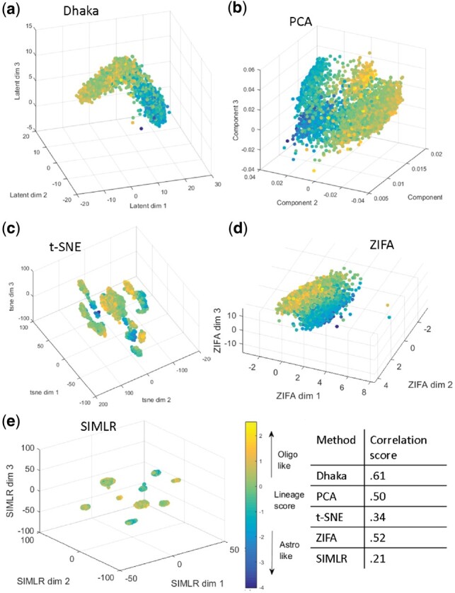
Comparison of Dhaka with PCA, t-SNE, ZIFA and SIMLR on Oligodendroglioma dataset with 5000 auto-selected genes. (a) Dhaka, (b) PCA, (c) t-SNE, (d) ZIFA, (e) SIMLR projections colored by lineage score. The Spearman rank correlation scores of the scoring metric (lineage and differentiation score) and the learned projections are shown in tabular form. We can see that Dhaka preserves the original scoring metric the best

3.4 Robustness analysis

A key issue with the analysis of scRNA-Seq data is dropout. In scRNA-Seq data we often see transcripts that are not detected even though the particular gene is expressed, which is known as the ‘dropout’. This happens mostly because of the low genomic quantity used for scRNA-Seq. We have tested the robustness of Dhaka to dropouts in the Oligodendroglioma dataset. We tested several different dropout percentages ranging from 0 to 50% (Supplementary Fig. S9a). Supplementary Figure S9c, e and g shows the histogram of dropout fractions of the genes in the dataset after artificially forcing 20, 30 and 50% more genes to be dropped out. Note that we cannot go beyond 50% in our analysis since several genes are already zero in the original data. Supplementary Figure S9b, d, f and h shows the projection of the Dhaka after adding 0, 20, 30 and 50% more drop out genes, respectively. We observe that when the additional drop-out rate is 30% or less, Dhaka can still retain the v-structure even though the cells are a bit more dispersed. At 50% we lose the v-structure, but the method can still separate oligo-like and astro-like cells even with this highly sparse data.

3.5 Analysis of marker genes in the Oligodendroglioma dataset

We further investigated the Dhaka learned structure to discover genes that are correlated with the lineages. To obtain trajectories for genes in the two lineages of the Oligodendroglioma dataset, we first segmented the Dhaka projected output into nine clusters using Gaussian mixture model (Fig. 5). Clusters 1–4 correspond to the oligo-branch and clusters −4 to −1 correspond to the astro-branch, while cluster 0 represents the bifurcation point. The choice to divide the cells into nine clusters is arbitrary to show the difference between the two branches. After computing the average expression profile of genes in the oligo and astro-branches, we performed two tailed t-test to identify differentially expressed genes among the group of cells in the two lineages. With Bonferroni corrected P-value <0.05, we find 1197 differentially expressed genes among 23 K original genes. We have also separately identified genes that are up regulated and down regulated in the two lineages (see list of genes in the supporting website). Expression profiles of a few of these genes are shown in Figure 5b–e. While a number of the genes found were known to be related to Oligodendroglioma pathway, many were only known to be related to other types of cancers or neurological disorders, but so far have not been associated with Oligodendroglioma. For example, TFG which is up regulated in the oligo-branch was previously affiliated in neuropathy (Ishiura et al., 2012). DDX39B gene is not directly related to cancer but is found to be localized near genes encoding for tumor necrosis factor α and β (Kikuta et al., 2012). Both HEXB and RGMA genes are up regulated in the astro-branch. These genes were previously identified in neurological disorders such as Sandhoff disease (Redonnet-Vernhet et al., 1996) and multiple sclerosis (Nohra et al., 2010), respectively. Our analysis suggests that they are key players in the Oligodendroglioma pathway as well.

Fig. 5.

New gene markers for astro-like and oligo-like lineages. (a) Segmenting autoencoder projected output to nine clusters. Clusters −4, −3, −2, −1 belongs to astro branch and clusters 1, 2, 3, 4 belong to oligo-branch. Cluster 0 represents the origin of bifurcation. (b–e) Expression profiles of couple of the top differntially expressed genes in the two lineages. (b) and (c) Up regulated in the oligo-branch, (d) and (e) up regulated in the astro-branch

3.6 Analysis of Glioblastoma data

The next dataset we looked at is the Glioblastoma dataset (Patel et al., 2014). This dataset contains 420 malignant cells with $\sim 6000$ expressed genes from six tumors. In this relatively small cohort of cells the authors did not find multiple subpopulations. However, they identified a stemness gradient across the cells from all six tumors (Patel et al., 2014), meaning the cells gradually evolve from a stem-like state to a more differentiated state. When we applied the Dhaka autoencoder to the expression profiles of the malignant cells, the cells were arranged in a chain like structure (Fig. 6a). To correlate the result with the underlying biology, we computed stemness score from the signature genes reported in the original paper (78 genes in total) (Patel et al., 2014). The score is computed as the ratio of average expression of the stemness signature genes to the average expression of all remaining genes (Patel et al., 2014). When we colored the scattered plot according to the corresponding stemness score of each cell, we see a chain like evolutionary structure where cells are gradually progressing form a stem-like state to a more differentiated state. As before, PCA, t-SNE, ZIFA, SIMLR, MAGIC, scvi and regular autoencoder projections (Fig. 6b–e, Supplementary Fig. S6a–d) fail to capture the underlying structure of this differentiation process. Only NMF can capture the linear trend in the data but results in much lower correlation score. We do see some outliers in Dhaka projections (blue dots near the yellow ones), however these outliers are similarly visible in results of other methods as well (Fig. 6). When we quantify the correlation of the Dhaka projection with the stemness score we can see that it clearly outperforms the other competing methods despite the outliers.

Fig. 6.

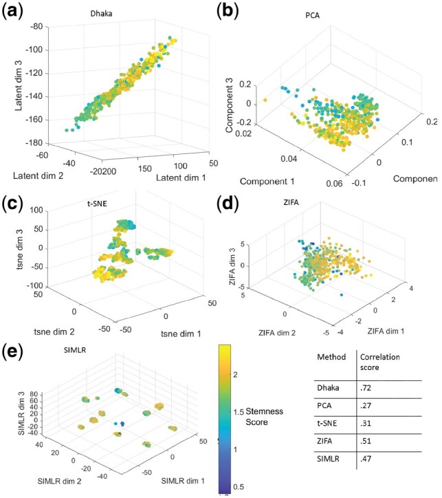
Comparison of Dhaka with PCA, t-SNE, ZIFA and SIMLR on Glioblastoma dataset. (a) Dhaka, (b) PCA, (c) t-SNE, (d) ZIFA, (e) SIMLR projections colored by stemness score. The Spearman rank correlation scores of the stemness score and the learned projections are shown in tabular form. We can clearly see that Dhaka preserves the original stemness score the best

After learning the structures we also wanted to see whether we can identify new marker genes for the stemness to differentiated program. For this, we reduced the latent dimension to 1 (since we see almost linear projection). Next, we computed Spearman rank correlation (Zar, 1998) of the 1D projection with every gene in the dataset. We have plotted a few of the top ranked positive (up regulated in the stem-like cells) and negative correlated genes (down regulated in the stem-like cells) (Fig. 7a). Despite the noisy expression profile, we do see a clear trend when a line is fitted (red). Among the discovered markers, TPT1 was identified as one of the key tumor proteins (Arcuri et al., 2004). Both RPS27 and TPT1 were found to be significant in other forms of cancer, such as Melanoma (Dai et al., 2010) and prostate cancer (Arcuri et al., 2004) and our results indicate that they may be involved in Glioblastoma as well. Among the down regulated genes, CLU was identified in the original paper (Patel et al., 2014) to be affiliated in Glioblastoma pathway whereas CANX was previously not identified as a marker for Glioblastoma. A complete list of correlated marker genes can be found in the supporting website.

Fig. 7.

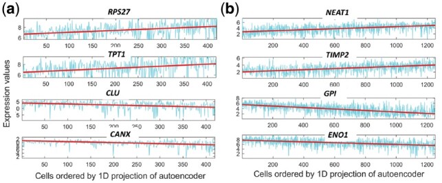
New marker gene: (a) Glioblastoma stemness program (b) Melanoma MITF-AXL program

3.7 Analysis of Melanoma data

The Melanoma cancer dataset (Tirosh et al., 2016a) profiled 1252 malignant cells with $\sim 23K$ genes from 19 samples. The expression values are log2 transformed transcript per million. When we used the relative expression values of 5000 auto-selected genes (based on $\overline{A}$ score) to the Dhaka autoencoder we saw two very distinct clusters of cells, revealing the intra-tumor heterogeneity of the Melanoma samples (Fig. 8a). In the original paper, the authors identified two expression programs related to MITF and AXL genes that give rise to a subset of cells that are less likely to respond to targeted therapy. The signature score for these programs were calculated by identifying genesets correlated with these two programs. The authors identified a total of 200 signature genes. We computed MITF-AXL signature score by computing the ratio of average expression of the signature genes and average expression of all remaining genes. When we colored the scattered plot with the MITF-AXL score, we indeed see that the clusters correspond to the MITF-AXL program, with one cluster scoring high and the other scoring low for these signature genes. Again, as can be seen from the figures and the correlation scores, such heterogeneity is not properly captured by t-SNE, PCA, ZIFA, SIMLR, MAGIC, NMF, regular autoencoder and scVI (Fig. 8b–e, Supplementary Fig. S6e–h).

Fig. 8.

Comparison of Dhaka with PCA, t-SNE, ZIFA and SIMLR on Melanoma dataset. (a) Dhaka, (b) PCA, (c) t-SNE, (d) ZIFA, (e) SIMLR projections colored by MITF-AXL score. The Spearman rank correlation scores with the scoring metric (MITF-AXL score) and Dhaka and the reported method projections are shown in tabular form. We can clearly see that Dhaka preserves the original MITF-AXL score the best

For this case too, we see almost a linear projection. To find new gene markers, we again computed 1D latent projection of the single cells and computed gene correlation. We have plotted a set of new marker genes both up and down regulated (Fig. 7b). The NEAT1 is a non-coding RNA, which acts as a transcriptional regulator for numerous genes, including some genes involved in cancer progression (Geirsson et al., 2003). TIMP2 gene plays a critical role in suppressing proliferation of endothelial cells and now we can see it is also relevant in the Melanoma cells (Vairaktaris et al., 2009). Among the down regulated genes, GPI functions as tumor-secreted cytokine and an angiogenic factor, which is very relevant to any cancer progression (Funasaka et al., 2001). The last correlated down regulated gene ENO1 is also known as tumor suppressor (Abu-Odeh et al., 2014). We have also looked whether the projection can recover some known gene marker dynamics or not. Four of the known gene markers are plotted in Supplementary Figure S8 (in Appendix). A complete set of gene markers can be found in the supporting website.

We also investigated whether Dhaka can capture the same trends in 2D projections as well. We have computed 2D projections of Oligodendroglioma, Glioblastoma and Melanoma (Supplementary Fig. S8). We can see that similar structure was captured in 2D projection as well. Although we see a decrease in correlation score for Glioblastoma and Melanoma.

We have also analyzed another scRNA-seq tumor dataset, Astrocytoma. For this dataset as well, Dhaka successfully separated malignant and non-malignant cells. It also correctly projected the cells in intermediate differentiation state as mentioned in the original paper of the dataset (Venteicher et al., 2017). Due to space constraint we have moved the analysis to the Appendix (Appendix 1.8, Supplementary Fig. S12).

3.8 CNV data

To test the generality of the method we also tested Dhaka with CNV data. We used copy number profiles from two xenograft breast tumor samples (xenograft 3 and 4, representing two consecutive time points) (Zahn et al., 2017). A total of 260 cells were profiled from xenograft 3 and 254 from xenograft 4. Both of these datasets have around 20 K genomic bin count. Cells were sequenced at a very low depth of 0.05X which results in noisy profiles. Copy numbers were estimated using a hidden Markov model (Wang et al., 2007). When we analyzed the copy number profile for xenograft 3, Dhaka identified one major cluster of cells and one minor cluster of cells (Fig. 9a). The identified clusters agree with the phylogenetic reconstruction analysis in the original paper. Figure 9b shows the copy number profiles of cells organized by phylogenetic analysis. Even though the copy number profiles are mostly similar in most parts of the genome, we do see that there is a small number of cells that have two copies (as opposed to one in the majority of cells, marked by red circle) in the x chromosome. Dhaka was able to correctly differentiate the minor cluster of cells from the rest. Next, we analyzed the xenograft 4 samples. The projected Dhaka output showed only one cluster which overlaps the major cluster identified for xenograft 3. We believe that the minor cluster from xenograft 3 probably did not progress further after serial passaging to the next mouse, whereas the major cluster persisted. This observation also agrees with the claim stated in the original paper (Zahn et al., 2017) that after serial passaging only one cluster remained in xenograft 4 which is a descendant of the major cluster in xenograft 3. We compared the copy number performance with other generalized methods as well, t-SNE, PCA, NMF and regular autoencoder (Supplementary Fig. S11). We can see that the separation between the major and minor clusters in xenograft 3 is most distinct in the projection from Dhaka. Also, the alignment of xenograft 4 cells with the major cluster from xenograft 3 is better preserved in Dhaka projection.

Fig. 9.

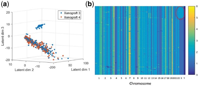
Dhaka output of two xenograft breast tumor samples’ copy number profile. (a) Identification of two subpopulations of cells in xenograft 3 and one subpopulation in xenograft 4. (b) Copy number profile of cells in xenograft 3 ordered by phylogenetic analysis, which shows that there are indeed two groups of cells present in the data (minor cluster having two copies of X chromosome marked by red circle). The colors correspond to the number of copies in each genomic bin count

4 Discussion

In this paper, we have proposed a new way of extracting useful features from single cell genomic data. The method is completely unsupervised and requires minimal pre-processing of the data. Using our method we were able to reconstruct lineage and differentiation ordering for several single cell tumor samples. Dhaka successfully separated oligo-like and astro-like cells along with their differentiation status for Oligodendroglioma scRNA-Seq data and has also successfully captured the differentiation trajectory of Glioblastoma cells. Similar results were obtained for Melanoma and Astrocytoma. Dhaka projections have also revealed several new marker genes for the cancer types analyzed. The method is general and can be applied to other types of genomic data as well. When applied to CNV data the method was able to identify heterogeneous tumor populations for breast cancer samples. In future, we will investigate larger single cell copy number datasets with more cells and more subpopulations.

An advantage of the Dhaka method is its ability to handle dropouts. Several single cell algorithms require pre-processing to explicitly model the drop-out rates. As we have shown, our method is robust and can handle very different rates eliminating the need to estimate this value.

We have shown results for two different output activation layers in our model, sigmoid and ReLU. Compared to sigmoid, ReLU activation function does not restrict the output between 0 and 1. Hence we see a lower reconstruction loss while training the autoencoder. However, the output projections using ReLU do not improve the resulting correlations with the biological scoring metrics. We present the results for ReLU activation in Supplementary Fig. S1. As can be seen, for the Oligodendroglioma and Glioblastoma datasets we obtain similar correlation scores for ReLU and sigmoid activation ($\pm 0.03$). However for the Melanoma and simulated datasets the scores for ReLU are lower (a difference >0.05), which means that these correlations are similar to the ones we obtain for the methods we compared to. While it is not entirely clear what leads to the improved performance of sigmoid, we hypothesize that it may be a function of the non-linear shape of the sigmoid function as opposed to the linear shape of ReLU. This may enable the sigmoid function to more strongly focus on significant genes which may be less noisy than the more balanced weights obtained by ReLU.

While our focus here was primarily on the identification of subpopulations and visualization, the latent representation generated by Dhaka could be used in pseudotime ordering algorithms as well (Setty et al., 2016; Trapnell et al., 2014). These methods often rely on t-SNE/PCA as the first step and replacing these with the Dhaka method is likely to yield more accurate results as we have shown. The VAE proposed here does not only cluster the cells, it can also represent an evolutionary trajectory, e.g. the V-structure for the Oligodendroglioma. Hence it can also be useful in phylogenetic analysis. Potential future work would focus on investigating the biological significance of the learned features and identifying key genes that align with the progression and mutations that help drive the different populations.

Funding

This work is supported by an internship at Microsoft Research.

Conflict of Interest: none declared.

References

- Abu-Odeh M. et al. (2014) Characterizing WW domain interactions of tumor suppressor WWOX reveals its association with multiprotein networks. J. Biol. Chem., 289, 8865–8880. [DOI] [PMC free article] [PubMed] [Google Scholar]
- Andor N. et al. (2016) Pan-cancer analysis of the extent and consequences of intra-tumor heterogeneity. Nat. Med., 22, 105.. [DOI] [PMC free article] [PubMed] [Google Scholar]
- Arcuri F. et al. (2004) Translationally controlled tumor protein (TCTP) in the human prostate and prostate cancer cells: expression, distribution, and calcium binding activity. Prostate, 60, 130–140. [DOI] [PubMed] [Google Scholar]
- Dai Y. et al. (2010) Extraribosomal function of metallopanstimulin-1: reducing paxillin in head and neck squamous cell carcinoma and inhibiting tumor growth. Int. J. Cancer, 126, 611–619. [DOI] [PubMed] [Google Scholar]
- de Bruin E.C. et al. (2014) Spatial and temporal diversity in genomic instability processes defines lung cancer evolution. Science, 346, 251–256. [DOI] [PMC free article] [PubMed] [Google Scholar]
- DeTomaso D., Yosef N. (2016) FastProject: a tool for low-dimensional analysis of single-cell RNA-Seq data. BMC Bioinformatics, 17, 315.. [DOI] [PMC free article] [PubMed] [Google Scholar]
- Fan J. et al. (2016) Characterizing transcriptional heterogeneity through pathway and gene set overdispersion analysis. Nat. Methods, 13, 241. [DOI] [PMC free article] [PubMed] [Google Scholar]
- Funasaka T. et al. (2001) Tumor autocrine motility factor is an angiogenic factor that stimulates endothelial cell motility. Biochem. Biophys. Res. Commun., 284, 1116–1125. [DOI] [PubMed] [Google Scholar]
- Gawad C. et al. (2016) Single-cell genome sequencing: current state of the science. Nat. Rev. Genet., 17, 175.. [DOI] [PubMed] [Google Scholar]
- Geirsson A. et al. (2003) Human trophoblast noncoding RNA suppresses CIITA promoter III activity in murine B-lymphocytes. Biochem. Biophys. Res. Commun., 301, 718–724. [DOI] [PubMed] [Google Scholar]
- Giustacchini A. et al. (2017) Single-cell transcriptomics uncovers distinct molecular signatures of stem cells in chronic myeloid leukemia. Nat. Med., 23, 692–702. [DOI] [PubMed] [Google Scholar]
- Gupta A. et al. (2015) Learning structure in gene expression data using deep architectures, with an application to gene clustering. In: Bioinformatics and Biomedicine (BIBM). pp. 1328–1335. IEEE.
- Hinton G.E., Salakhutdinov R.R. (2006) Reducing the dimensionality of data with neural networks. Science, 313, 504–507. [DOI] [PubMed] [Google Scholar]
- Ishiura H. et al. (2012) The TRK-fused gene is mutated in hereditary motor and sensory neuropathy with proximal dominant involvement. Am. J. Hum. Genet., 91, 320–329. [DOI] [PMC free article] [PubMed] [Google Scholar]
- Jolliffe I.T. (1986) Principal component analysis and factor analysis. In: Principal Component Analysis. Springer, New York, pp. 115–128. [Google Scholar]
- Joyce J.M. (2011) Kullback-Leibler divergence. In: International Encyclopedia of Statistical Science. Springer, New York, pp. 720–722. [Google Scholar]
- Kikuta K. et al. (2012) Clinical proteomics identified ATP-dependent RNA helicase DDX39 as a novel biomarker to predict poor prognosis of patients with gastrointestinal stromal tumor. J. Proteomics, 75, 1089–1098. [DOI] [PubMed] [Google Scholar]
- Kingma D.P., Welling M. (2013) Auto-encoding variational Bayes. arXivv, 1312, 6114. [Google Scholar]
- LeCun Y. et al. (2015) Deep learning. Nature, 521, 436–444. [DOI] [PubMed] [Google Scholar]
- Lee D.D., Seung H.S. (2001) Algorithms for non-negative matrix factorization. In: Advances in Neural Information Processing Systems, pp. 556–562.
- Li X. et al. (2017) Network embedding-based representation learning for single cell RNA-seq data. Nucleic Acids Res., 45, e166.. [DOI] [PMC free article] [PubMed] [Google Scholar]
- Lin C. et al. (2017) Using neural networks for reducing the dimensions of single-cell RNA-seq data. Nucleic Acids Res., 45, e156. [DOI] [PMC free article] [PubMed] [Google Scholar]
- Lopez R. et al. (2017) A deep generative model for single-cell RNA sequencing with application to detecting differentially expressed genes. arXiv, 1710, 05086. [Google Scholar]
- Maaten L.v.d., Hinton G. (2008) Visualizing data using t-SNE. J. Mach. Learn. Res., 9, 2579–2605. [Google Scholar]
- Min J.-W. et al. (2015) Identification of Distinct Tumor Subpopulations in Lung Adenocarcinoma via Single-Cell RNA-seq. PLoS One, 10, e0135817.. [DOI] [PMC free article] [PubMed] [Google Scholar]
- Navin N.E., Hicks J. (2010) Tracing the tumor lineage. Mol. Oncol., 4, 267–283. [DOI] [PMC free article] [PubMed] [Google Scholar]
- Nohra R. et al. (2010) RGMA and IL21R show association with experimental inflammation and multiple sclerosis. Genes Immun., 11, 279–293. [DOI] [PubMed] [Google Scholar]
- Patel A.P. et al. (2014) Single-cell RNA-seq highlights intratumoral heterogeneity in primary glioblastoma. Science, 344, 1396–1401. [DOI] [PMC free article] [PubMed] [Google Scholar]
- Pierson E., Yau C. (2015) ZIFA: dimensionality reduction for zero-inflated single-cell gene expression analysis. Genome Biol., 16, 241.. [DOI] [PMC free article] [PubMed] [Google Scholar]
- Redonnet-Vernhet I. et al. (1996) Significance of two point mutations present in each HEXB allele of patients with adult GM2 gangliosidosis (sandhoff disease) homozygosity for the Ile207 Val substitution is not associated with a clinical or biochemical phenotype. Biochim. Biophys. Acta, 1317, 127–133. [DOI] [PubMed] [Google Scholar]
- Roweis S.T., Saul L.K. (2000) Nonlinear dimensionality reduction by locally linear embedding. Science, 290, 2323–2326. [DOI] [PubMed] [Google Scholar]
- Russnes H.G. et al. (2011) Insight into the heterogeneity of breast cancer through next-generation sequencing. J. Clin. Invest., 121, 3810.. [DOI] [PMC free article] [PubMed] [Google Scholar]
- Setty M. et al. (2016) Wishbone identifies bifurcating developmental trajectories from single-cell data. Nat. Biotechnol., 34, 637–645. [DOI] [PMC free article] [PubMed] [Google Scholar]
- Tieleman T., Hinton G. (2012) Lecture 6.5-rmsprop: divide the gradient by a running average of its recent magnitude. In: COURSERA: Neural Networks for Machine Learning. Coursera, Mountain View, California, Vol. 4, pp. 26–31. [Google Scholar]
- Tirosh I. et al. (2016a) Dissecting the multicellular ecosystem of metastatic melanoma by single-cell RNA-seq. Science, 352, 189–196. [DOI] [PMC free article] [PubMed] [Google Scholar]
- Tirosh I. et al. (2016b) Single-cell RNA-seq supports a developmental hierarchy in human oligodendroglioma. Nature, 539, 309–313. [DOI] [PMC free article] [PubMed] [Google Scholar]
- Trapnell C. et al. (2014) The dynamics and regulators of cell fate decisions are revealed by pseudotemporal ordering of single cells. Nat. Biotechnol., 32, 381–386. [DOI] [PMC free article] [PubMed] [Google Scholar]
- Vairaktaris E. et al. (2009) Gene polymorphisms related to angiogenesis, inflammation and thrombosis that influence risk for oral cancer. Oral Oncol., 45, 247–253. [DOI] [PubMed] [Google Scholar]
- van Dijk D. et al. (2017) MAGIC: a diffusion-based imputation method reveals gene-gene interactions in single-cell RNA-sequencing data. BioRxiv, 111591. [Google Scholar]
- Venteicher A.S. et al. (2017) Decoupling genetics, lineages, and microenvironment in IDH-mutant gliomas by single-cell RNA-seq. Science, 355, eaai8478.. [DOI] [PMC free article] [PubMed] [Google Scholar]
- Wang B. et al. (2017) Visualization and analysis of single-cell RNA-seq data by kernel-based similarity learning. Nat. Methods, 14, 414–416. [DOI] [PubMed] [Google Scholar]
- Wang K. et al. (2007) PennCNV: an integrated hidden Markov model designed for high-resolution copy number variation detection in whole-genome SNP genotyping data. Genome Res., 17, 1665–1674. [DOI] [PMC free article] [PubMed] [Google Scholar]
- Xu C., Su Z. (2015) Identification of cell types from single-cell transcriptomes using a novel clustering method. Bioinformatics, 31, 1974–1980. [DOI] [PMC free article] [PubMed] [Google Scholar]
- Zahn H. et al. (2017) Scalable whole-genome single-cell library preparation without preamplification. Nat. Methods, 14, 167–173. [DOI] [PubMed] [Google Scholar]
- Zar J.H. (1998) Spearman rank correlation. In: Peter,A. and Theodore,C. (eds) Encyclopedia of Biostatistics. John Wiley & Sons, Hoboken, NJ. [Google Scholar]
- Zong C. et al. (2012) Genome-wide detection of single-nucleotide and copy-number variations of a single human cell. Science, 338, 1622–1626. [DOI] [PMC free article] [PubMed] [Google Scholar]
Associated Data
This section collects any data citations, data availability statements, or supplementary materials included in this article.