PINet: Privileged Information Improve the Interpretablity and generalization of structural MRI in Alzheimer’s Disease

Abstract

The irreversible and progressive atrophy by Alzheimer’s Disease resulted in continuous decline in thinking and behavioral skills. To date, CNN classifiers were widely applied to assist the early diagnosis of AD and its associated abnormal structures. However, most existing black-box CNN classifiers relied heavily on the limited MRI scans, and used little domain knowledge from the previous clinical findings. In this study, we proposed a framework, named as PINet, to consider the previous domain knowledge as a Privileged Information (PI), and open the black-box in the prediction process. The input domain knowledge guides the neural network to learn representative features and introduced intepretability for further analysis. PINet used a Transformer-like fusion module Privileged Information Fusion (PIF) to iteratively calculate the correlation of the features between image features and PI features, and project the features into a latent space for classification. The Pyramid Feature Visualization (PFV) module served as a verification to highlight the significant features on the input images. PINet was suitable for neuro-imaging tasks and we demonstrated its application in Alzheimer’s Disease using structural MRI scans from ADNI dataset. During the experiments, we employed the abnormal brain structures such as the Hippocampus as the PI, trained the model with the data from 1.5T scanners and tested from 3T scanners. The F1-score showed that PINet was more robust in transferring to a new dataset, with approximatedly 2% drop (from 0.9471 to 0.9231), while the baseline CNN methods had a 29% drop (from 0.8679 to 0.6154). The performance of PINet was relied on the selection of the domain knowledge as the PI. Our best model was trained under the guidance of 12 selected ROIs, major in the structures of Temporal Lobe and Occipital Lobe. In summary, PINet considered the domain knowledge as the PI to train the CNN model, and the selected PI introduced both interpretability and generalization ability to the black box CNN classifiers.

1. Introduction

The lack of interpretability and generalization remained the major problems when applying CNN classifiers to medical image analysis. Currently, the general pipeline was to train a CNN model and generate the salience map based on the model. [1], [2], [3], [4]. Such pipeline heavily relied on the data and were lack of clinical meanings, which caused “overfitting issue” as most medical images had small number of image data. The CNN models can achieve promising performance in a specific dataset from one hospital but failed dramatically in other datasets, which may due to a slight collecting bias such as using 3T scanners instead of 1.5T scanners for MRI scans. Given the poor generalizability, their conclusions were not convincing for clinicians. For the second deflects, current available methods relied heavily on dataset itself, without considering domain knowledge from clinical studies or clinicians, which could lead to trivial findings with little medical meaning. As a result, the salience map from the model was capture confounding bias instead of the real cause of the abnormal brain structures. To overcome the above issues and identify interpretable features in AD, we proposed a stable and robust framework PINet to include the previous medical findings as Privileged Information (PI), which guides neural network to learn representative features. As clinicians can put forward different domain knowledge via PI, our PINet was able to explain the results and thus improved the interpretability to the black-box CNN classifiers. To demonstrate the capability of PINet, we applied it to predict the diagnosis of Alzheimer’s Disease through structural MRI scans. Alzheimer’s Disease (AD) caused brain atrophy and loss of cells, resulting in a continuous decline in thinking and behavioral skills. The control was denoted as the Cognitively Normal (CN) group. To date, CNN-based methods were widely applied in the early diagnosis of AD. [5], [6]. The early work of AD classifiers focused on improving the accuracy without focusing on the interpretablity [7], [8], [9].These models were using single modality and was sensitive to the dataset. To improve the generalization ability of the CNN model, previous work enlarged the dataset with EMR [10], [11], functional MRI (FMRI) [12], positron emission tomography (PET) [10], [13] and Image genetic data as additional dataset. These multi-modality model reported multiple brain areas with strong relationships with the potential cause of AD. Venugopalan et al. [11] found abnormal structure in the brain area of hippocampus, amygdala. Zhang et al. [[14]] reported significant different in the brain area of Cerebellum. But the multi-modality methods were constrained by the missing data ACM-BCB, September 3–6, 2023, Houston, TX Double Blind for submission from the dataset. For example, a patient had only MRI scans, and another patient had only PET images. Therefore, the multi-modality approaches were limited to the missing data issues. Meanwhile, findings from clinical ends reported significant difference in particular brain structural [15], [16], [17], [18], [19], [20], [21], [22] [23] [24]. The findings used statistic methods rather than CNN-based models, and interpret the abnormal brain structures with clinical meanings. Thus, our motivation was using these domain knowledge as the a strong guidance, and “teach” the neural network to converge into the desired directions with more medical meaning features. We denoted this prior domain knowledge as the Privileged Information (PI), and proposed the PINet to address the influence of the PI in training a robust model. PINet allowed the clinicians to manually control the guidance domain knowledge, which served as the key to open the black box of CNN models. In this context, the PI improved the interpretability of the models. PINet added two components to the standard CNN classifiers: (1) A Privileged Information Fusion (PIF) module to address the connections between the image features and the PI features. (2) A Pyramid Feature visualization (PFV) module to highlight significance features on the inputs and verify the effect of the PI features. To avoid the confounding bias such as the hard device from scanners (1.5T or 3T), in the experiment, PINet showed a better generalization ability than the baseline CNN models. The performance of PINet relied on the quality of the domain knowledge, and a confusing set of the PI can mislead the model and ended up with bad results. And PINet can be used as a discriminator to find the suitable set of the PI when the causes of the disease were unclear. Our main contribution can be summarized as the following three points:(1) Proposed a Privileged Information Fusion (PIF) module to fuse the PI in model training. PIF can reflect the influence of the PI and showed a more stable performance when transferring from 1.5T dataset to 3T dataset. (2) PINet served as discriminator to determine the correctness of PI. If the PI cannot reflect the potential cause of neuro-imaging, PINet was not able to converge. Hence it can used as a framework to find a suitable subset of PI. (3) Introduced a Pyramid Feature Visualization (PFV) approach. Compare with the previous methods, PFV can capture more informative brain structures.

2. METHODS

2.1. PINet Overview

As shown in Figure 1, the PINet forward the Input MRI data and Privileged Information (PI) into a CNN for feature extraction, and fused the image features and PI features via Privileged Information Fusion (PIF) and classified the latent features into AD or CN group. As a classifier, PINet was designed for N categories (N = 2 in the experiment). PINet proposed two components: Privileged Information Fusion (PIF) and Pyramid Feature Visualization (PFV). PIF was an add-on component to address the influence of the PI features and guide the model to learn representative image features. PVF was a visualization module to highlight the significant features into the input images, and reflected the impact of the PI in the prediction process.

Figure 1:

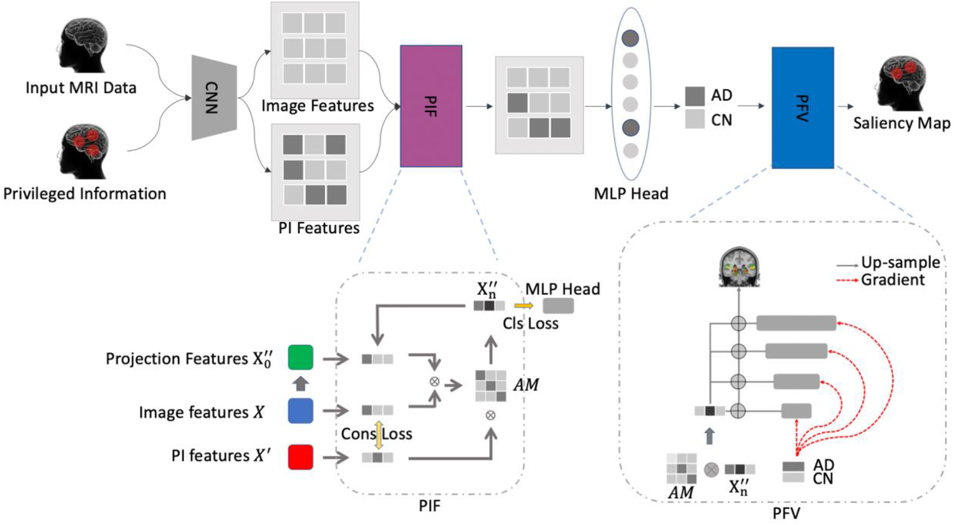
Overview of PINet. The network had considered the input MRI data and the domain knowledge as the Privileged Information. The image and PI features were fused via our proposed module Privileged Information Fusion (PIF), and project the latent space and put forward the MLP head for prediction. The Privileged Feature Visualization (PFV) module generated informative salience map and highlight the contributing features on the MRI inputs.

2.2. Privileged Information Fusion (PIF)

The CNN models learnt a mapping between the input data (e.g. the MRI scans) X and target ground truth (e.g. classification labels) y with a heuristic function (e.g. the backbone parameters of the neural network) with parameters $h_w(.)$ .A loss function $ℒ$ helped minimized the gap between the prediction and the ground truth:

$${\text{min}}_w{E}_{(X,y)~p(X,y)}[ℒ(y,h(X\mid w))]$$

Privileged information (PI)[25] from previous clinical findings was introduced as additional input that guided the neural network to converge to the desired direction and to learn interpretable features with clinical meaning. Here we introduced the PI (denoted as $X\prime$) in the training process as:

$${\text{min}}_w{E}_{\left(X,X^{\prime },y\right)~p(X,X^{\prime },y)}\left[ℒ\left(y,h\left(X,X^{\prime }\mid w\right)\right)\right]$$

In PINet, we used a backbone network to extract the image features (X) and corresponding PI features ($X\prime$). We project the image features (X) into a latent space $X_0^{″}$, and iterative update the projection features with attention mechanism R. We denoted the i-th iteration of updating the projection features as $X_i^{″}$. To encourage the network to learn the features as PI, we generated a consistency loss ${ℒ}_{\mathit{\text{cons}}}$, where $h_{\theta }$ was the model to extract the features from input data and privileged information. The consistency loss served as a “noise” filter to strengthen the features from privileged information.

$${ℒ}_{\mathit{\text{cons}}}=\left|\right|h_w(X)-h_w\left(X^{\prime }\right)|{|}_1$$

The consistency loss was a regularization to encourage the image features learn more similarity from the PI features. To address the connection between the image features and the PI features, we employed a “Transformer-like” structure to fuse the PI features into the image features, and project the fused features into a latent space for classification. We initialized the projection features $X_0^{″}$ using a two layer MLP as a “warm up”. Rather than putting forward the $X_0^{″}$ into a classification head, which is a standard CNN classifier, we calculated the association between image features X and projection features $X_0^{″}$, generated an attention map (AM) R, and then updated the new projection features $X_1^{″}$ by multiplying the PI features $X\prime$. The computation process was repeated for n times, and the final projection features $X_n^{″}$ was put forward to a classification head for the final prediction. We denoted each update of the projection features as one iteration. The whole fusion process was the Transformer-like structure with the image features serving as the key component K, PI features serving as the value component V, and the latent features in the projection space serveing as Query Q. In this way, we calculated the relevance Matrix R for updating the project features (denotation) via a cross-view transformer structure:

$$R_{ij}=<\frac{{x^{″}}_{ni}}{‖{x^{″}}_{ni}‖},\frac{x_j}{‖{\text{x}}_{\text{j}}‖}>$$

$${X^{″}}_{n+1}=\text{Softmax}(R)\left(X^{\prime }\right)$$

where n was the n-th iteration in the feature fusion process. The final latent projection features predicted the results $p_c$ with a MLP classification head. Finally, we updated the weights of X, $X\prime$ and $X_n^{″}$ with an end-to-end framework with a supervised cross-entropy loss:

$${ℒ}_{\mathit{\text{cls}}}=\frac{1}{N}\sum _i\sum _c^N\left(y_{ic}\mathit{\text{log}}\left(p_{ic}\right)\right.$$

The $y_{ic}$ and $p_{ic}$ represented for the class of the ith item of ground truth and prediction, respectively. And we have the total loss function as

$$ℒ=\alpha {ℒ}_{\mathit{\text{cls}}}+\beta {ℒ}_{\mathit{\text{cons}}}$$

2.3. Pyramid Feature Visualization (PFV)

PFV was inspired by feature pyramid network and gradient-based CAM. As figure 2 was shown, the original grad-cam had to up-sampling a large scale of regions before highlighting the features on the original data. All the visualization filtered the background and only kept the positions in particular brain areas. After filtering the guided back-propagation methods, only a few voxels overlayed with the original data. In comparison, our proposed Pyramid Feature Visualization (PFV) provided a trade-off between the up-sampling CAM and the guided gradients from the input data.

Figure 2:

Comparison of visualization methods using the structure of the left and right Hippocampus as reference. Our proposed visualization methods were able to capture informative structures while the vanilla saliency map capture irrelevant brain structures, and other methods had only a few points and lost the brain structures.

The original GradCam was represented by the following:

$${\text{GradCam}}_c=\text{ReLU}\left(\sum _k\sum _i\sum _j\frac{\partial y_c}{\partial f_{ij}^k}{f}^k(X)\right)$$

where $f_{ij}^k$ was the feature in the position of (i,j) in the kth feature map, and $f^k\left(X\right)$ was the output of the kth feature map. In our PFV, we presented pyramid gradient maps(PGM) in each down-sampling stages. The PGM were shown via the red dot lines in Figure 1. The idea was that up-sampling features will interpolate with adjacent features, while few of the features were contributing to the prediction. And aggregating the gradient maps from each down-sampling stage can serve as a refinement of highlighting the contributing features. In addition, gently aggregating the gradient maps can also capture the adjacent features with relatively small gradients. On the contrary, if we directly up-sampling the feature map back to the original size, say 32 times, the irrelevant voxels in the nearby brain areas were also captured, and the highlight areas will be too wide.

$${\text{PGM}}_c=\sum _s{\alpha }_s{\text{GradCam}}_c^s$$

For our investigation specifically, PVF also evaluated the features that were selected from attention maps. We produced the Pyramid Attention Maps (PAM) as an attribute to indicate the significant features from neural networks and treat it as an additional filter rule in selecting the features:

$$\text{PAM}=\sum _{\text{i}}{X}_i^{″}\cdot R\cdot X_i^{\prime }$$

In summary, the attention map reflected the effect from PI features$X\prime$, while the gradient maps showed the influence from original image features X. The final visualization from PFV was a weighted combination of the two contributing salience maps:

$$\text{PFV}={\alpha }_1\text{PGM}+{\alpha }_2\text{PAM}$$

3. Results and discussion

3.1. Dataset and Implementation

In this study, we used the dataset from ADNI (adni.loni.usc.edu) dataset. In training and validation, we used data from 1.5T scanners with at least one year of screening from the date of clinically confirmed diagnosis. In testing, we collected data from 3T scanners with at least one year of screening from confirmed diagnosis. In total, we collected 590 instances for training and validation, with 236 AD instances, 354 cognitively normal (CN) instances in the training set, and 55 AD, 95 CN in the validation set. In the testing set, we collected 44 instances with 13 AD and 31 CN. All the instances were pre-processed with the standard registration from FSL with a MNI-152-1mm template, and the input size was 182 × 218 × 182. We removed the artifacts from background using the the from FSL. PINet was trained with 40 epoches, with learning rate lr = 1e⁻⁴, and AdamW optimizer. We saved the weights in Nifti format and visualized them using the tools in FSL (A UI tool named as fsleyes), which can screenshot and saved as png format. In FSL, we set the minimum threshold as min = 0.54 and the maximum threshold as max = 0.58, and used “ACTC” color bar to highlight the features.

3.2. Quantitative Results

We built up a CNN baseline and perform an ablation study to verify how different combinations of privilege information affected the results. The comparison used the same training/validation/testing set with the same backbone networks (ResNet-10). In all the experiments, we were using the positions of ROIs from AAL3 templates as the PI. AAL3 was the third version of the automated anatomical atlas, which provided an alternative parcellation to describe the individual functions of each brain structure in MNI-152 space. AAL3 divided the brain structures into 170 subparts, each of which indicated a unique brain structure. In our experiments, we first employed the total 170 ROIs as the and trained a model from scratch. As shown in Table 1, compared with the CNN baseline without the PIF component, the model trained with had better performance in both the validation set and testing set. In particular, we found the drop rate of transferring from 1.5T to 3T dataset was 13% in our proposed model, while the drop rate was 29% in the CNN baseline. Note that we have removed the background artifacts, using all the ROIs from the AAL3 template was equivalent to adding attention modules to address the relations among the brain areas. In this case, the improvement was from adding a Transformer-like module into the original CNN structures. The difference was that the vanilla CNN structures considered the distance of all brain areas evenly, but the attention mechanism took one more step and considered the distances among brain areas differently, which was making more sense and thus improved the performance. The next step was to evaluate the effect of the selection from different PI. Here we presented two series of experiments: (1) fine-tuning from the model using 170 ROIs. (2) Trained from the scratch model directly. In the first experiment, we compared two different selections of privileged information. We exported the top K mean weights of the brain areas from the validating set and selected the same K brain areas based on the previous findings. In our experiment, we choose K = 12 ROIs. (The range of the weights were in [0.5, 0.61], and we have 11 weights that were larger than 0.6. Since the brain should be symmetric, therefore we chose K=12 for a even number.) The top 12 ROIs from the model was: The left part of (weight=0.6123), the left part of Pallidum (weight=0.6115), the left and right part of Thalamus (weight=0.609, 0.609), the left and right part of Lateral Geniculate Nucleus of Thalamus (weight=0.6085, 0.6017), the left part of Putamen (weight=0.6071), the left part of Pulvinar Nuclei of Thalamus (weight=0.6055), the left part of Amygdala (weight=0.6036), the left part and right part of Hippocampus (weight=0.6024, 0.6994) and the left part of Caudate(weight=0.6012). Similarly, we selected 12 ROIs as the following: the left and right part of Hippocampus, the left and right part of Para Hippocampal, the left and right part of Amygdala, the left and right part of Occipital Superior, the left and right part of Temporal Superior and the left and right part of Temporal Pole Superior. Both fine-tuned models had better performance than the model trained with 170 ROIs, showing that using less but more accurate PI can have a slight improvement. When it came to the drop rate of transferring the model to the testing set, we can find using findings from previous literature (drop rate=2.56%) were more robust than using the top 12 ROIs from the model purely based on the data (drop rate=10.95%).

Table1:

Comparative Results and performance of ablation Study

methods	Validation Set					Testing Set
	AD/CN	Accuracy	Sen	Spe	F1	AD/CN	Accuracy	Sen	Spe	F1
CNN Baseline	55/95	0.9067	0.8364	0.9474	0.8679	13/31	0.7727	0.6154	0.8387	0.6154
+ PIF (170 ROIs)	55/95	0.9467	0.8909	0.9789	0.9245	13/31	0.8864	0.7692	0.9355	0.8000
Pretrain (170 ROIs) + Selected (12 ROIs)	55/95	0.9600	0.9818	0.9474	0.9474	13/31	0.9545	0.9231	0.9677	0.9231
Pretrain(170 ROIs) + Top (12 ROIs)	55/95	0.9533	0.9273	0.9684	0.9358	13/31	0.9091	0.7692	0.9677	0.8333
Top (12 ROIs)	55/95	0.9200	0.8545	0.9569	0.8868	13/31	0.8182	0.4615	0.9677	0.6000
Selected (12 ROIs)	55/95	0.8533	0.8909	0.8316	0.8167	13/31	0.8409	0.9231	0.8065	0.7742

Furthermore, we trained the model from scratch with the same settings of PI. The goal of this set of experiments was to evaluate the performance of the model with the limited information. As we mentioned above, PINet can serve as a discriminator to examine whether the PI was correct or not. If we address the misleading knowledge, it would guide the network in the wrong direction and therefore the network would end up with very bad performance or even not convergence. On the contrary, if the PI was correct, the model should still converge and had similar performance in the validation set and testing set. The performance of the two sets of PI was shown in Table 1, and the drop rate of the model using selected 12 ROIs remained low (drop rate = 4%), but the drop rate of the model using top 12 ROIs were increasing (drop rate = 32%).

We went through the implicit reason for the increased drop rate when training the top 12 ROIs from scratch. As Figure 3 illustrated, we sorted the mean of the contributing weights of each brain area using the prediction in the validation set. And we matched the position of the top 12 ROIs and the selected 12 ROIs into the position, The figure showed that all the selected ROIs had relatively high weights (the smallest weight was 0.5764) from the pre-trained model with 170 ROIs. The illustration indicated that the model trained with 170 ROIs had noticed the influence from the selected 12 ROIs. But the dataset may exist a few confounding biases and therefore other ROIs could be more important in the particular dataset. In this case, fine-tuning with the previous findings was addressing the influence of the selected ROIs in the prediction of the diagnosis results, and the correct ROIs were also the dominant features in the 3T dataset, which resulted in a robust prediction in the test data. On the contrary, when trained from scratch, PI with top 12 ROIs had better performance in the validation set, but much worse performance in the testing set. The phenomenon could explain the difference of our proposed PINet with previous CNN classifiers. The previous CNN classifiers relied heavily on the dataset and identified the “top 12 ROIs” as the influence brain areas. Though the performance in the validation set was better, the results were not stable in transferring into a new dataset, the 3T testing dataset in our case. On the contrary, PINet can produce more robust performance in both validation set and testing set. On one hand, we have worse F1 scores in the validation set, but we can have similar results in transferring to the testing set with a slight performance drop.

Figure 3:

The blue bar chart was the descending weight of all 170 ROIs of the model with all ROIs as the PI. We compared the weights of ROI of the top 12 ROIs and the selected 12 ROIs. This figure showed that the selected 12 ROIs had relatively high weights in all 170 ROIs when all of them were used in the prediction.

3.3. Visualization Results

In this section, we presented the visualization results of PINet. To date, previous works had employed multiple visualization tools, including CAMs, guided GradCAM, DeepLift and Graident-Shap. In Figure 2 We generated the heatmap using the above-mentioned algorithm in a standard MNI152-1mm human brain template. However, the generated heatmap was either covering too spacious brain areas or too sparse. For example, the guided GradCAM, DeepLift, and Gradient-Shap only generated a few sparse points on the input data, which hardly captured the structure of the ROIs. In contrast, the salience map covered more than half of the brain areas, introducing too many irrelevant ROIs.

Therefore, inspired by FPN, we came up with the idea of upsampling and aggregating the pyramid of each gradient map to generate a heatmap that can capture the relevant brain structures. Compared to the previous approaches, our proposed methods were able to capture the entire structure of both the left and right part of the Hippocampus.

Moreover, we compared the heatmap from PFV with the PI with 170 ROIs, top 12 ROIs, and selected 12 ROIs, shown in Figure 4 we also illustrated the origin input from one of the participants who was unfortunately confirmed as an AD patient. We used two red circles to crop the corresponding position in the input area to indicate the brain atrophy in the brain area of Hippocampus. In this example, the brain atrophy was obvious from the perspective of Axial and all of the three models were able to capture this atrophy structure. In comparison, with the same threshold from the range of [0.54,0.58], the visualization model using 170 ROIs as the PI had split the weights evenly and results in capturing too many ROIs. In contrast, the rest two models with 12 ROIs as the PI were able to focus more on the highly influenced regions in the position of the left and right part of Hippocampus. Note that this part was in the PI of both the top 12 ROIs and selected 12 ROIs, therefore this figure indicated that the model can learn from the guidance of the PI.

Figure 4:

We compared visualization results from the model with 170 ROIs, top 12 ROIs and selected 12 ROIs as the PI. The heat map was overlapped into the original inputs from Axial, Coronal and Sagittal views. The red circles in the axial view crop the abnormal brain structure in the left and right part of the Hippocampus. All three models were able to capture the structural difference, but the models using the selected 12 ROIs can capture more precise brain structures than the rest two.

3.4. Interpret via Privileged Information

PINet can serve as a discriminator to validate the performance of the PI when it was unknown. Our assumption was that model with correct PI was able to converge, otherwise, the model cannot converge to a satisfying result. Therefore, based on AAL-VOI categories, we roughly divided the brain areas into 7 groups: Temporal Lobe (TL), Posteriror Fossa (PF), Insula and Cingulate Gyrus (ICG), Frontal Lobe (FL), Occipital Lobe (OL), Parietal Lobe (PL), and Central Structures (CS). And we applied each of the categories as the PI and trained the neural network from scratch. In the experiment, we mainly focused on whether the model can converge and we trained 20 epochs for each set of the PI. From the experiments, three of the categories: Temporal Lobe (TL), Occipital Lobe (OL) and Central Structures (CS) was able to converge and the performance of using the ROIs in Temporal Lobe (TL) was much better than the rest two set. We then implement two more experiments using the combination of TL + OL and TL + OL + CS. The performance was similar to the model results using all 170 ROIs. In addition, the position of selected 12 ROIs located in and OL and the position of top 12 ROIs was located in TL and CS. The experiment results showed that the structures in Temporal Lobe, Occipital Lobe and Central Structures were related to the potential cause of Alzheimer’s Disease.

4. Conclusion

In this investigation, we proposed a framework to make use of the Privileged Information to guide the neural network to learn representative features and robust in performance when transferring to a new dataset. We introduced a Privileged Information Fusion (PIF) module to combine the PI into the prediction process of a neural network. As we can control the input of the PI, we are able to teach the neural network to learn the desired features as we want. The framework can be easily extended to other neuro-imaging applications, especially when the biomarkers were known while the data were limited and had confounding bias. Furthermore, we introduced a pyramid feature visualization method and can generate an informative heatmap compared to previous visualization approaches. In summary, PINet provided a general interpretable framework and assisted the clinicians to put forward their domain knowledge into the computation of medical imaging.

Table2:

Explore Brain structures based on AAL-VOI categories

methods	Validation Set					Testing Set
	AD/CN	Acc	Sen	Spe	F1	AD/CN	Acc	Sen	Spe	F1
TL	55/95	0.9000	0.8727	0.9158	0.8649	13/31	0.9091	0.8462	0.9355	0.8462
PF	55/95	0.6467	0.0364	1.000	0.0702	13/31	0.7045	0.0000	1.000	0.0000
ICG	55/95	0.6333	0.0000	1.000	0.0000	13/31	0.7045	0.0000	1.000	0.0000
FL	55/95	0.6400	0.0545	0.9789	0.1000	13/31	0.6818	0.1538	0.9032	0.2222
OL	55/95	0.8533	0.8364	0.8632	0.8070	13/31	0.7272	0.7692	0.7097	0.6250
PL	55/95	0.6333	0.0000	1.000	0.0000	13/31	0.7045	0.000	1.000	0.0000
CS	55/95	0.7400	0.5091	0.8737	0.5895	13/31	0.8182	0.3846	1.000	0.5556
TL + OL	55/95	0.9400	0.9273	0.9474	0.9189	13/31	0.9091	0.9231	0.9032	0.8571
TL + OL + CS	55/95	0.9467	0.9636	0.9368	0.9298	13/31	0.9318	0.9231	0.9355	0.8889

CCS CONCEPTS.

• Applied computing → Bioinformatics.

REFERENCES

- 1.Lundberg SM and Lee S-I, A unified approach to interpreting model predictions. Advances in neural information processing systems, 2017. 30. [Google Scholar]
- 2.Selvaraju RR, et al. Grad-cam: Visual explanations from deep networks via gradient-based localization. in Proceedings of the IEEE international conference on computer vision. 2017. [Google Scholar]
- 3.Shrikumar A, Greenside P, and Kundaje A. Learning important features through propagating activation differences. in International conference on machine learning. [Google Scholar]
- 4.Zhou B, et al. Learning deep features for discriminative localization. in Proceedings of the IEEE conference on computer vision and pattern recognition. [Google Scholar]
- 5.Noor MBT, et al. , Application of deep learning in detecting neurological disorders from magnetic resonance images: a survey on the detection of Alzheimer’s disease, Parkinson’s disease and schizophrenia. Brain informatics, 2020. 7(1): p. 1–21–1–21. [DOI] [PMC free article] [PubMed] [Google Scholar]
- 6.Yamanakkanavar N, Choi JY, and Lee B, MRI segmentation and classification of human brain using deep learning for diagnosis of Alzheimer’s disease: a survey. Sensors, 2020. 20(11): p. 3243–3243. [DOI] [PMC free article] [PubMed] [Google Scholar]
- 7.Gupta A, Ayhan M, and Maida A. Natural image bases to represent neuroimaging data. in International conference on machine learning. [Google Scholar]
- 8.Hosseini-Asl E, Gimel’farb G, and El-Baz A, Alzheimer’s disease diagnostics by a deeply supervised adaptable 3D convolutional network. arXiv preprint arXiv:1607.00556, 2016. [DOI] [PubMed] [Google Scholar]
- 9.Payan A and Montana G, Predicting Alzheimer’s disease: a neuroimaging study with 3D convolutional neural networks. arXiv preprint arXiv:1502.02506, 2015. [Google Scholar]
- 10.Liu Y, et al. , Incomplete multi-modal representation learning for Alzheimer’s disease diagnosis. Medical Image Analysis, 2021. 69: p. 101953–101953. [DOI] [PubMed] [Google Scholar]
- 11.Venugopalan J, et al. , Multimodal deep learning models for early detection of Alzheimer’s disease stage. Scientific reports, 2021. 11(1): p. 1–13–1–13. [DOI] [PMC free article] [PubMed] [Google Scholar]
- 12.Yang F, et al. Disentangled Sequential Graph Autoencoder for Preclinical Alzheimer’s Disease Characterizations from ADNI Study. in International Conference on Medical Image Computing and Computer-Assisted Intervention. [Google Scholar]
- 13.Zhou B, et al. Synthesizing Multi-tracer PET Images for Alzheimer’s Disease Patients Using a 3D Unified Anatomy-Aware Cyclic Adversarial Network. in International Conference on Medical Image Computing and Computer-Assisted Intervention. [Google Scholar]
- 14.Zhang Y, et al. , Detection of subjects and brain regions related to Alzheimer’s disease using 3D MRI scans based on eigenbrain and machine learning. Frontiers in computational neuroscience, 2015. 9: p. 66–66. [DOI] [PMC free article] [PubMed] [Google Scholar]
- 15.Dronse J, et al. , In vivo patterns of tau pathology, amyloid-β burden, and neuronal dysfunction in clinical variants of Alzheimer’s disease. Journal of Alzheimer’s disease, 2017. 55(2): p. 465–471–465–471. [DOI] [PubMed] [Google Scholar]
- 16.Galton CJ, et al. , Atypical and typical presentations of Alzheimer’s disease: a clinical, neuropsychological, neuroimaging and pathological study of 13 cases. Brain, 2000. 123(3): p. 484–498–484–498. [DOI] [PubMed] [Google Scholar]
- 17.Harasty JA, et al. , Specific temporoparietal gyral atrophy reflects the pattern of language dissolution in Alzheimer’s disease. Brain, 1999. 122(4): p. 675–686–675–686. [DOI] [PubMed] [Google Scholar]
- 18.Madhavan A, et al. , FDG PET and MRI in logopenic primary progressive aphasia versus dementia of the Alzheimer’s type. PloS one, 2013. 8(4): p. e62471–e62471. [DOI] [PMC free article] [PubMed] [Google Scholar]
- 19.Nasrallah IM, et al. , 18F-Flortaucipir PET/MRI correlations in nonamnestic and amnestic variants of Alzheimer disease. Journal of Nuclear Medicine, 2018. 59(2): p. 299–306–299–306. [DOI] [PMC free article] [PubMed] [Google Scholar]
- 20.Ossenkoppele R, et al. , Tau PET patterns mirror clinical and neuroanatomical variability in Alzheimer’s disease. Brain, 2016. 139(5): p. 1551–1567–1551–1567. [DOI] [PMC free article] [PubMed] [Google Scholar]
- 21.Tetzloff KA, et al. , Regional distribution, asymmetry, and clinical correlates of tau uptake on [18F] AV-1451 PET in atypical Alzheimer’s disease. Journal of Alzheimer’s Disease, 2018. 62(4): p. 1713–1724–1713–1724. [DOI] [PMC free article] [PubMed] [Google Scholar]
- 22.Whitwell JL, et al. , Imaging correlates of posterior cortical atrophy. Neurobiology of aging, 2007. 28(7): p. 1051–1061–1051–1061. [DOI] [PMC free article] [PubMed] [Google Scholar]
- 23.Whitwell JL, et al. , Temporoparietal atrophy: a marker of AD pathology independent of clinical diagnosis. Neurobiology of aging, 2011. 32(9): p. 1531–1541–1531–1541. [DOI] [PMC free article] [PubMed] [Google Scholar]
- 24.Xia C, et al. , Association of in vivo [18F] AV-1451 tau PET imaging results with cortical atrophy and symptoms in typical and atypical Alzheimer disease. JAMA neurology, 2017. 74(4): p. 427–436–427–436. [DOI] [PMC free article] [PubMed] [Google Scholar]
- 25.Lambert J, Sener O, and Savarese S. Deep learning under privileged information using heteroscedastic dropout. in Proceedings of the IEEE Conference on Computer Vision and Pattern Recognition. 2018. [Google Scholar]