Spiking neural networks for nonlinear regression

Abstract

Spiking neural networks (SNN), also often referred to as the third generation of neural networks, carry the potential for a massive reduction in memory and energy consumption over traditional, second-generation neural networks. Inspired by the undisputed efficiency of the human brain, they introduce temporal and neuronal sparsity, which can be exploited by next-generation neuromorphic hardware. Energy efficiency plays a crucial role in many engineering applications, for instance, in structural health monitoring. Machine learning in engineering contexts, especially in data-driven mechanics, focuses on regression. While regression with SNN has already been discussed in a variety of publications, in this contribution, we provide a novel formulation for its accuracy and energy efficiency. In particular, a network topology for decoding binary spike trains to real numbers is introduced, using the membrane potential of spiking neurons. Several different spiking neural architectures, ranging from simple spiking feed-forward to complex spiking long short-term memory neural networks, are derived. Since the proposed architectures do not contain any dense layers, they exploit the full potential of SNN in terms of energy efficiency. At the same time, the accuracy of the proposed SNN architectures is demonstrated by numerical examples, namely different material models. Linear and nonlinear, as well as history-dependent material models, are examined. While this contribution focuses on mechanical examples, the interested reader may regress any custom function by adapting the published source code.

1. Introduction

In recent years, artificial neural networks (ANN) have gained much attention in the computational engineering sciences and applied mathematics due to their flexibility and universal approximation capabilities, both for functions [1,2] and operators [3]. Their outstanding but surprising generalizability capabilities are yet to be understood [4]. Their advantages have been used in a variety of applications, including fluid dynamics [5–9], solid mechanics [10–13], micromechanics [14–17], material parameter identification [18–22], constitutive modelling [23–26], fracture mechanics [27,28], microstructure generation [29–31], contact problems [32–35], heat transfer [36–39], uncertainty quantification [40–43], among numerous others. Refer to [44–46] for review publications.

Despite the success of ANNs, several problems arise alongside their use, such as the need for high-frequency memory access, which leads to high computational power demand [47,48]. This results in huge costs for training and often makes it preferable to run inference in remote servers during deployment. In general, ANNs are most often trained on graphics processing units (GPUs), whose energy consumption is problematic in embedded systems (e.g. sensor devices) as is required in automotive and aerospace applications [49] or structural health monitoring (SHM). Furthermore, high latency during prediction time can arise where acceleration or parallelization is not available. Figure 1 illustrates a potential use case of neuromorphic hardware in SHM. Using concepts from data-driven mechanics, sensor data collected during service life may be interpreted with the aid of high-dimensional (computational) physical models, which so far have only been used to design infrastructures or products. Thanks to active research, the computational efficiency of such advanced monitoring concepts is rapidly increasing (e.g. [50], for a recent contribution). A bottleneck for practical online applications, however, remains the aforementioned hardware constraints, namely, energy demand and latency. Regression using spiking neural networks (SNN) on neuromorphic hardware may contribute to overcome persisting limitations.

Figure 1.

SNN-based regression offers high potential in many energy-critical applications, such as SHM. We expect that, thanks to the advent of data-driven modelling, it will become possible to interpret sensor data directly where it is recorded on neuromorphic hardware as part of embedded devices. Current work is concerned with the solution of partial differential equations on neuromorphic hardware, which will ultimately allow to evaluate and update computational models online.

Originally motivated by the human brain, today’s traditional ANN architectures are an oversimplification of biology, relying on dense matrix multiplication. From a numerical and computational hardware point of view, dense matrix multiplication is often suboptimal. Sparsity is thought to be favourable as it reduces dependence on memory access and data communication [51]. In contrast, the human brain is much more efficient, where neurons are considered to be sparsely activated [52]. This stems from the fact that the brain uses sparse electronic signals for information transmission instead of dense activations. This leads to remarkable capabilities by using only approximately 10–20 W of energy. One attempt to overcome these drawbacks of ANNs is to introduce the information transmission mechanism of biological neurons into network architectures. These networks are called SNN due to the electronic impulses or spikes used for communication between neurons [53]. This leads to sparse activations, which can be efficiently exploited by neuromorphic hardware, such as Loihi [54], SpiNNaker [55] and TrueNorth [56]. It has been shown that these specialized hardware chips can reduce the energy consumption of neural network-based processes by factors of up to ×1000 [54,57–60]. Apart from their energy efficiency in prediction, recent attempts to increase the training efficiency of SNN can be found in [61–64].

What was classically in the domain of neuroscientists recently has been investigated in the context of deep learning, for example, the adoption of SNNs to supervised learning as popularized with traditional ANNs in frameworks, such as TensorFlow [65] and PyTorch [66], resulting in similar frameworks for spiking deep learning like snnTorch [67]. Some applications of spiking deep learning include image processing using a spiking ResNet [68] and temporal data processing using spiking long short-term memory neural network (SLSTM) variants [69,70]. A combination of spiking convolutional neural networks and LSTMs was proposed in Yang et al. [71]. SNNs have been used for image segmentation [72] and localization [73,74].

To the best of the authors’ knowledge, the full potential of energy-efficient regression modelling using SNNs has up to now not yet been fully exploited. In Iannella and Back [75], an architecture using inter-spike interval temporal encoding has been proposed, where the functions learned were limited to piecewise constant functions. In Gehrig et al. [76], a SNN was used for the regression of angular velocities of a rotating event camera. Building on these results, Rançon et al. [77] proposed a SNN for depth reconstruction. Both works rely on fully connected decoders for real-valued output, which increases the energy demand compared with an architecture relying only on SNN predictions. This is due to the increased number of dense matrix multiplications in fully connected layers. In Kahana et al. [78], a DeepONet [79] using SNN was proposed, which used a floating point decoding scheme to regress simple one-dimensional functions. This decoding scheme led to non-smooth and staircase-like predictions. In Shrestha and Orchard [80], gradient descent was applied to learn spike times. Here, as in the present contribution, the membrane potential is used, but to tweak the occurrence of the first spikes in the SNN. In Eshraghian et al. [81], classification problems using the membrane potential in the context of memristor-based hardware were explored, but no regression tasks. Recently, a SNN has been proposed in a computational mechanics context in Tandale and Stoffel [82], which builds up on our approach developed in the preprint [83]. However, again fully connected layers were added, which counteract the energy efficiency.

The focus of the present work lies on network architectures that come along without any fully connected layers and are therefore optimally suited for neuromorphic hardware, which is specifically designed for SNNs. The proposed regression approach works without fully connected dense encoders/decoders by using only spiking layers. The output of the proposed networks is real-valued, continuous functions and can represent highly nonlinear, history-dependent data accurately.

As regression problems are omnipresent in engineering sciences, a flexible and broadly applicable framework would enable SNNs to be used in a variety of engineering applications and further unfold the potential of neuromorphic hardware. To this end, the present study aims towards the following key contributions:

• — Introduction of spiking neural networks. Concise introduction of this emerging technique. Open source benchmark code for the research community, fostering further developments of SNN in mechanics and applied mathematics (see also Data accessibility section).
• — History-dependent regression framework. We demonstrate that SNNs can model systems that exhibit hysteresis, thus history-dependent behaviour. We present a flexible framework to use SNNs in complex regression tasks, demonstrated by means of a nonlinear material model, namely isotropic hardening plasticity.
• — Efficiency, sparsity and latency. We benchmark our SNN for neuromorphic hardware in terms of memory and energy consumption as compared with non-spiking equivalent networks, demonstrating that our approach is much more efficient with respect to memory and power consumption, making neural networks more sustainable. This is enabled by a membrane potential-based decoding scheme, which does not rely on fully connected decoders. While in our study an emulator is used, deployment on neuromorphic hardware allows highly efficient usage in embedded environments.

The present work intends to introduce this important novel technique to the community of computational mechanics and applied mathematics. To concentrate on the novelties and to keep the presentation concise, we restrict ourselves to one-dimensional regression problems. However, the framework is not restricted to single-variable regression and is easily applicable to a multi-variable regression.

The remainder of this article is structured as follows. In §2, the basic notations of SNNs are derived from traditional ANNs. A simple spiking counterpart to the classical densely connected feed-forward neural network is introduced. After that, our regression SNN topology is proposed. Starting with a linear regression example (linear elasticity), we point out the problems arising in SNN regression. This basic architecture is extended towards recurrent feedback loops in §3. The ability of these recurrent SNNs is showcased on a nonlinear material model. To process history-dependent regression tasks with dependencies over a large number of time steps, a spiking LSTM is introduced in §4. An application to a history-dependent plasticity model shows that SNNs can achieve similar accuracy as their traditional counterparts while being much more efficient. The paper closes with a conclusion and an outlook towards future research directions in §5. For the code accompanying this manuscript, see the Data accessibility section at the end of this manuscript.

2. Spiking neural networks for regression

SNNs are considered to be the third generation of neural networks. While the first generation was restricted to shallow networks, the second generation is characterized by deep architectures. A broad use of second-generation neural networks has been enabled by the availability of automatic differentiation and software frameworks such as TensorFlow [65]. To introduce SNN, we compare them with their well-known second-generation counterparts.

2.1. Second-generation neural networks

An ANN is a parametrized, nonlinear function composition. The universal function approximation theorem [1] states that arbitrary Borel measurable functions can be approximated with ANNs. There are several different architectures for ANNs, for example, feed-forward, recurrent or convolutional networks, which can be found in standard references such as [84–88]. Following Hauser [89], most ANN formulations can be unified. An ANN ${\displaystyle \mathcal{N}}$ , more precisely, a densely connected feed-forward neural network, is a function from an input space ${\displaystyle {\mathbb{R}}^{d_x}}$ to an output space ${\displaystyle {\mathbb{R}}^{d_y}}$ , defined by a composition of nonlinear functions ${\displaystyle {\mathit{h}}^{(l)}}$ , such that

$${\displaystyle {\displaystyle \begin{array}{rl}\mathcal{N}:{\mathbb{R}}^{d_x}& \to {\mathbb{R}}^{d_y}\\ \mathit{x}& \mapsto \mathcal{N}(\mathit{x})={\mathit{h}}^{(l)}\circ \dots \circ {\mathit{h}}^{(0)}=\mathit{y},\\ l& =1,\dots ,n_L.\end{array}}}$$ (2.1)

Here, x denotes an input vector of dimension ${\displaystyle d_x}$ and y an output vector of dimension ${\displaystyle d_y}$ . The nonlinear functions ${\displaystyle {\mathit{h}}^{(l)}}$ are called layers and define an ${\displaystyle l}$ -fold composition, mapping input vectors to output vectors. Consequently, the first layer ${\displaystyle {\mathit{h}}^{(0)}}$ is defined as the input layer and the last layer ${\displaystyle {\mathit{h}}^{(n_L)}}$ as the output layer, such that

$${\displaystyle {\displaystyle {\mathit{h}}^{(0)}=\mathit{x}\in {\mathbb{R}}^{d_x},{\mathit{h}}^{(n_L)}=\mathit{y}\in {\mathbb{R}}^{d_y}.}}$$ (2.2)

The layers ${\displaystyle {\mathit{h}}^{(l)}}$ between the input and output layers, called hidden layers, are defined as

$${\displaystyle {\displaystyle \begin{array}{rl}{\mathit{h}}^{(l)}& =\left\{h_{\eta }^{(l)},\eta =1,\dots ,n_u\right\},\\ h_{\eta }^{(l)}& ={\varphi }^{(l)}\left({\mathit{W}}_{\eta }^{(l)}{\mathit{h}}^{(l-1)}\right),\end{array}}}$$ (2.3)

where ${\displaystyle h_{\eta }^{(l)}}$ is the n-th neural unit of the l-th layer ${\displaystyle {\mathit{h}}^{(l)}}$ , ${\displaystyle n_u}$ denotes the total number of neural units per layer, ${\displaystyle {\mathit{W}}_{\eta }^{(l)}}$ is the weight vector of the n-th neural unit in the l-th layer ${\displaystyle {\mathit{h}}^{(l)}}$ and ${\displaystyle {\mathit{h}}^{(l-1)}}$ is the output of the preceding layer, where bias terms are absorbed [86]. Furthermore, ${\displaystyle {\varphi }^{(l)}:\mathbb{R}\to \mathbb{R}}$ is a nonlinear activation function. All weight vectors ${\displaystyle {\mathit{W}}_{\eta }^{(l)}}$ of all layers ${\displaystyle {\mathit{h}}^{(l)}}$ can be gathered in a single expression, such that

$${\displaystyle {\displaystyle {\mathit{\theta }}_{\text{ANN}}=\left\{{\mathit{W}}_{\eta }^{(l)}\right\},}}$$ (2.4)

where ${\displaystyle \mathit{\theta }}$ inherits all parameters of the ANN ${\displaystyle \mathcal{N}(\mathit{x})}$ from equation (2.1). Consequently, the notation ${\displaystyle \mathcal{N}(\mathit{x};\mathit{\theta })}$ emphasizes the dependency of the outcome of an ANN on the input on one hand and the current realization of the weights on the other hand. The specific combination of layers ${\displaystyle {\mathit{h}}^{(l)}}$ from equation (2.3), neural units ${\displaystyle h_{\eta }^{(l)}}$ and activation functions ${\displaystyle {\varphi }^{(l)}}$ from equation (2.3) is called the topology of the ANN ${\displaystyle \mathcal{N}(\mathit{x};\mathit{\theta })}$ . The weights θ from equation (2.4) are typically found by gradient-based optimization with respect to a task-specific loss function [85]. An illustration of a densely connected feed-forward ANN is shown in figure 2.

Figure 2.

Densely connected feed-forward neural network topology of an ANN ${\displaystyle \mathcal{N}(\mathit{x};\mathit{\theta })}$ as described in equation (2.1).

It can be seen that the ANN described in equation (2.1) takes an input and produces an output, one at a time. If history-dependent input and output data and are considered, the formulation of the hidden layers reads

$$\begin{gathered} {\displaystyle {\mathit{h}}_t^{(l)}=\left\{h_{\eta ,t}^{(l)},\eta =1,...,n_u,t=0,...d_t\right\}, \\ {h}_{\eta ,t}^{(l)}={\varphi }^{(l)}({\mathit{W}}_{\eta }^{(l)}{h}_t^{\left(l-1\right)}),} \end{gathered}$$ (2.5)

where the time component is discrete. This can be understood as processing each discrete-time slice of the input vector of the preceding layer ${\displaystyle {\mathit{h}}_{t=0}^{(l-1)}\to {\mathit{h}}_{t=1}^{(l-1)}\to ,...,\to {\mathit{h}}_{t=d_t}^{(l-1)}}$ sequentially, where the weights ${\displaystyle {\mathit{W}}_{\eta }^{(l)}}$ are shared over all time steps. At this stage, the formulation in equation (2.5) is purely notational, as there is no connection of the weights through different time steps.

2.2. Spiking neural networks

A SNN can be seen as a history-dependent ANN, which introduces memory effects by means of biologically inspired processes. Standard works in theoretical neuroscience include the studies of Dayan and Abbott [90], Izhikevich [91] and Gerstner et al. [92]. Several overviews of SNNs with respect to deep learning can be found in [93–95].

To this end, the activation function ${\displaystyle {\varphi }^{(l)}}$ in equation (2.5) can be formulated as

$${\displaystyle {\displaystyle \begin{array}{r}{\varphi }_{\text{spk},t}^{(l)}=\{\begin{array}{l}1,U_{\eta ,t}^{(l)}\ge U_{\text{thr},\eta }^{(l)}\\ 0,U_{\eta ,t}^{(l)}<U_{\text{thr},\eta }^{(l)},\end{array}\end{array}}}$$ (2.6)

with

$${\displaystyle U_{\eta ,t}^{(l)}={\beta }_{\eta }^{(l)}{U}_{\eta ,t-1}^{(l)}+{\mathit{W}}_{\eta }^{(l)}{\mathit{h}}_t^{(l-1)}-{\varphi }_{\text{spk},t-1}^{(l)}{U}_{\text{thr},\eta }^{(l)},}$$ (2.7)

where ${\displaystyle U_{\eta ,t}^{(l)}}$ is the membrane potential of the ${\displaystyle \eta }$ -th neural unit at time ${\displaystyle t}$ , ${\displaystyle U_{\text{thr},\eta }^{(l)}}$ denotes the membrane threshold, ${\displaystyle {\beta }_{\eta }^{(l)}}$ is the membrane potential decay rate and ${\displaystyle {\mathit{W}}_{\eta }^{(l)}{\mathit{h}}_t^{(l-1)}}$ is the standard ANN weight multiplied with the preceding layer of the current time step, respectively, see equation (2.5). Basically, the SNN activation restricts the neural unit to output discrete pulses ${\displaystyle ({\varphi }_{\text{spk}}=1)}$ if the membrane threshold is reached by the time-evolving membrane potential, or to remains silent ${\displaystyle ({\varphi }_{\text{spk}}=0)}$ . These pulses are called spikes, see Figure 3. The last summand in equation (2.6), ${\displaystyle -{\varphi }_{\text{spk},t-1}^{(l)}{U}_{\text{thr},\eta }^{(l)}}$ , is called the reset mechanism and resets the membrane potential by the threshold potential once a spike is emitted. The membrane threshold and membrane potential decay rate can be optimized during training, such that the optimization parameters of a SNN are

Figure 3.

Spiking neuron dynamics. Input spikes ${\displaystyle {\varphi }_{\mathrm{s}\mathrm{p}\mathrm{k}}^{i,0}}$ trigger changes in the membrane potential ${\displaystyle U^1}$ , which when sufficiently excited beyond a threshold ${\displaystyle U_{\mathrm{t}\mathrm{h}\mathrm{r}}}$ causes the neuron to emit an output spike ${\displaystyle {\varphi }_{\mathrm{s}\mathrm{p}\mathrm{k}}^{j,1}}$ .

$${\displaystyle {\displaystyle {\mathit{\theta }}_{\text{SNN}}=\left\{{\mathit{W}}_{\eta }^{(l)},{\beta }_{\eta }^{(l)},U_{\text{thr},\eta }^{(l)}\right\}.}}$$ (2.8)

The SNN formulation in equation (2.7) is called the leaky integrate and fire (LIF) neuron model, and is one of the most widely used models in spike-based deep learning. It can be seen as the baseline SNN and plays a similar role as densely connected feed-forward ANN in classical deep learning. Equation (2.7) can also be interpreted as the explicit forward Euler solution of an ordinary differential equation, describing the time variation of the membrane potential, see Eshraghian et al. [67] for details.

The main difference between SNNs and classical ANNs lies in the way information is processed and propagated through the network from neuron to neuron. In standard ANNs, inputs, hidden layers and output vectors are handled via dense matrices. In SNN, sparsity is introduced by using spikes, which are single events expressed via a Dirac delta function or a discrete pulse in continuous or discrete settings, respectively. A group of spikes over time is called a spike train ${\displaystyle \mathit{i}=\left[i_t,t=0,...,n_t\right]}$ . To this end, a spiking neuron is subjected to a spike train over a time interval, consisting of spikes (1) or zero input (0). The membrane potential ${\displaystyle U_{\eta ,t}^{(l)}}$ is modulated with incoming spikes ${\displaystyle i_t}$ . In the absence of input spikes, the membrane voltage decays over time due to the membrane decay rate ${\displaystyle {\beta }_{\eta }^{(l)}}$ . The absence of spikes introduces sparsity because, in every time step, the neural unit output is constrained to either 0 or 1. This fact can be exploited on neuromorphic hardware, where memory and synaptic weights need only be accessed if a spike is apparent. Otherwise, no information is transmitted. In contrast, conventional ANNs do not leverage sparsely activated neurons, and most deep learning accelerators, such as GPUs or tensor processing units (TPUs), are correspondingly not optimized for it.

2.3. Spiking neural networks training

Unfortunately, the spiking activation ${\displaystyle {\varphi }_{\text{spk},t}^{(l)}}$ in equation (2.6) is non-differentiable. To use the backpropagation algorithm from standard ANNs, the activation is replaced using a surrogate gradient during the backward pass. Several different formulations have been proposed (e.g. [51,96,97]). In this work, the arcus tangent surrogate activation from Fang et al. [98] is used,

$${\displaystyle {\displaystyle {\varphi }_{\text{surr}}\left(x\right)=\frac{1}{\pi }\arctan \left(\pi x\right),{\varphi }_{\text{surr}}^{\prime }\left(x\right)=\frac{1}{1+{\left(\pi x\right)}^2},}}$$ (2.9)

for some input ${\displaystyle x}$ . The surrogate ${\displaystyle {\varphi }_{\text{surr}}\left(x\right)}$ is continuously differentiable and preserves the gradient dynamics of the network. Thus, for training using backpropagation and its variants, ${\displaystyle {\varphi }_{\text{surr}}^{\mathrm{\prime }}}$ is employed. Illustrations can be found in figures 4 and 5.

Figure 4.

Computational graph of an unrolled SNN. Forward pass.

Figure 5.

Computational graph of an unrolled SNN. Backward pass.

2.4. Network topology

The key question for using SNN in regression is how to transform real input values into binary spikes and binary spike information at the output layer back to real numbers. The former task is called spike encoding, whereas the latter is called spike decoding. Popular forms of encoding include rate encoding, latency encoding, delta modulation, among others. Similarly, different decoding strategies exist, such as rate decoding and latency decoding. An illustration of various encoding and decoding strategies is shown in figure 6. Refer to Eshraghian et al. [67] for an overview and detailed description. In this work, a constant current injection is chosen for the encoding part, whereas a novel population voting on membrane potential approach is chosen for the decoding part. It will be demonstrated throughout the numerical examples that, with the proposed spike decoding scheme, accurate and efficient SNN regression is made possible.

Figure 6.

A sample of spike-based encoding and decoding strategies. (a): Real-valued inputs are encoded into spikes by means of different strategies [67], for example: (i) high intensities or large values result in a large number of spikes (top left); (ii) high intensities or large values result in early spike firing (centre left); and (iii) delta modulation where spikes are produced for positive gradients of the input function (bottom left). (b): In classification, the predicted class is determined via (i) the number of spikes (top right) or (ii) the first occurrence of spikes (bottom right). Regression is introduced in §2.2.

All network topologies used in the upcoming numerical examples follow a general scheme, which is flexible and suited for regression tasks. First, the real input ${\displaystyle {\mathit{x}}_t}$ is provided as a constant input to the first layer ${\displaystyle {\mathit{h}}_t^{(0)}}$ , for all time steps t, such that

$${\displaystyle {\displaystyle {\mathit{h}}_t^{(0)}\left({\mathit{x}}_t\right)={\mathit{h}}_t^{\text{const}}\left({\mathit{x}}_t\right)={\mathit{x}}_t\mathrm{\forall }t\in \left[0,d_t\right].}}$$ (2.10)

Then, several SNN layers ${\displaystyle {\mathit{h}}_t^{(l)}}$ follow, where the exact formulation will be given for every numerical example. The output of the last spiking layer ${\displaystyle {\mathit{h}}_t^{(n_L)}}$ is transformed into a decoding layer ${\displaystyle {\mathit{h}}_t^{\text{dec}}}$ , which takes the membrane potential of every time step as input and outputs real numbers

$${\displaystyle {\displaystyle {\mathit{h}}_t^{\text{dec}}={\beta }_{\eta }^{(l)}{U}_{\eta ,t-1}^{(l)}+{\mathit{W}}_{\eta }^{(l)}{\mathit{h}}_t^{(l-1)},}}$$ (2.11)

which is essentially the formulation of equation (2.7), where no spikes and reset mechanisms are used. The transformed values are then transferred to a ‘population voting layer’, where the output of all neurons of the decoding layer are averaged to give real numbers. This results in

$${\displaystyle {\displaystyle h_t^{\mathtt{p}\mathtt{o}\mathtt{p}}=\frac{1}{n_o}\sum _{n_o}\left({\beta }_n^{(l)}{U}_{\eta ,t-1}^{(l)}+W_n^{(l)}{h}_n^{(l-1)}\right),}}$$ (2.12)

where n _o denotes the number of neurons in the population voting layer and again, no spikes or reset mechanisms are used.

The final spiking regression topology network ${\displaystyle \mathcal{S}}$ can be written as

$${\displaystyle {\displaystyle \begin{array}{rlr}\mathcal{S}:{\mathbb{R}}^{d_t\times d_x}& \to {\mathbb{R}}^{d_t\times d_y}& \\ {\mathit{x}}_t& \mapsto {\mathit{h}}_t^{\text{pop}}\circ {\mathit{h}}_t^{\text{dec}}\circ {\mathit{h}}_t^{(n_L)}\circ \dots \circ {\mathit{h}}_t^{(l)}\circ \dots & \\ & \dots \circ {\mathit{h}}_t^{(1)}\circ {\mathit{h}}_t^{\text{const}}\left({\mathit{x}}_t\right)={\mathit{y}}_t.& \end{array}}}$$ (2.13)

To summarize, information flows in the following form:

• —The input layer ${\displaystyle {\mathit{h}}_t^{\text{const}}={\mathit{x}}_t}$ equation (2.10) takes constant current (real numbers ${\displaystyle {\mathit{x}}_t}$ ).
• —The input is then transformed into binary spikes in the spiking layers ${\displaystyle {\mathit{h}}_t^{(l)}}$ (equation (2.6))
• —and transformed back into real numbers in the translation layer ${\displaystyle {\mathit{h}}_t^{\text{dec}}}$ Equation (2.11)().
• —The output is formed in the population layer ${\displaystyle {\mathit{h}}_t^{\text{pop}}}$ Equation (2.12).

A graphical interpretation is given in figure 7.

Figure 7.

Topology of the spiking regression network is introduced in §2.1.

For all the following numerical examples, the AdamW optimizer from Loshchilov and Hutter [99] is used. The parameters are set as follows: learning rate ${\displaystyle \alpha =1\times {10}^{-3}}$ , exponential decay rates for the first- and second-moment estimates ${\displaystyle {\beta }_1=0.9}$ and ${\displaystyle {\beta }_2=0.999}$ , respectively, weight decay ${\displaystyle \lambda =0.01}$ . The training was carried out on a Nvidia GeForce RTX 3090 GPU using snnTorch [67] and PyTorch [66]. In this work, the mean relative error ${\displaystyle \mathcal{E}}$ is used, which is defined as

$${\displaystyle {\displaystyle {\mathcal{E}}_{\bullet }(\bullet )=\frac{1}{n_s}{\displaystyle \sum _{i=1}^{n_s}\frac{||{\hat{\bullet }}_i-{\bullet }_i|{|}_2}{||{\hat{\bullet }}_i|{|}_2},}}}$$ (2.14)

for some input ${\displaystyle \bullet }$ and baseline ${\displaystyle \hat{\bullet }}$ . If the error is reported for all time steps, ${\displaystyle \bullet }$ is a vector containing the values of all time steps. If the error is reported for the last time step, ${\displaystyle \bullet }$ is equal to the last component of the corresponding history-dependent vector.

2.5. Numerical experiment: linear regression

We first study the performance of the proposed LIF topology in a simple linear regression problem. To this end, the general model described in §2.1 with LIF defined in equation (2.7) is used, resulting in the following network topology.

$${\displaystyle {\displaystyle \mathcal{S}\left({\epsilon }_t\right)={\mathit{h}}_t^{\text{pop}}\circ {\mathit{h}}_t^{\text{dec}}\circ {\mathit{h}}_t^{\text{LIF}}\circ {\mathit{h}}_t^{\text{LIF}}\circ {\mathit{h}}_t^{\text{LIF}}\circ {\mathit{h}}_t^{\text{const}}\left({\epsilon }_t\right)={\sigma }_t.}}$$ (2.15)

To begin with, a simple linear elastic material model with strains in the range of ${\displaystyle \epsilon =[0,0.001]}$ and fixed Young’s modulus ${\displaystyle E=2.1\times {10}^5}$ MPa is considered, such that the resulting stress ${\displaystyle \sigma }$ is

$${\displaystyle {\displaystyle \sigma =E\epsilon .}}$$ (2.16)

The training data consists of strain input, uniformly sampled in the interval ${\displaystyle \epsilon =[0,0.001]}$ , and stress output calculated according to equation (2.16). Three datasets are generated from equation (2.16), namely, training set, validation set and test set consisting each of ${\displaystyle n_{\text{train}}=n_{\text{val}}=n_{\text{test}}=1024}$ samples. All three datasets are standardized using the mean and standard deviation from the training set. The batch size is chosen as ${\displaystyle n_{\text{batch}}=1024}$ . The number of neurons ${\displaystyle n_u}$ is chosen as ${\displaystyle n_u=128}$ and is kept constant over all layers. The training is carried out for ${\displaystyle 2\times {10}^3}$ epochs. The model performing best on the validation set is chosen for subsequent evaluations. The mean relative error accumulated over all time steps and the mean relative error of the last time step with respect to the test set are reported.

Although the linear regression problem is a time-independent problem, SNN has an inherent time dependency. Instead of time, the SNN is thus trained on a sequence of strain steps ${\displaystyle \mathrm{\Delta }\epsilon }$ . We investigate the effect of the number of strain (time) steps on the prediction accuracy, with results illustrated in figure 8.

Figure 8.

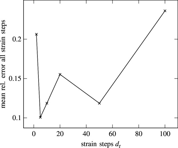
Elasticity—error of all strain (time) steps. Mean relative error for all strain steps with respect to the different total number of strain steps. The error is rising for a larger number of strain steps.

It can be seen that the mean relative error is lowest for ${\displaystyle d_t=5}$ strain steps. For ${\displaystyle d_t=2}$ , the error is larger. This could be caused by a lack of a sufficient number of strain steps for the neuron dynamics to effectively be calculated. It can be understood as a failure due to too large strain steps in the explicit stepping scheme in equation (2.7). Clearly, the highest error can be observed for ${\displaystyle d_t=100}$ strain steps. In contrast, as depicted in figure 9, the error at the last strain step is lowest for ${\displaystyle d_t=100}$ strain steps. To illustrate the cause, the prediction of the network for two different samples, one for ${\displaystyle d_t=5}$ and one for ${\displaystyle d_t=100}$ strain steps are shown in figures 10 and 11, respectively. While good agreement on the endpoints is apparent, fluctuation during the rest of the strain steps causes the error to rise. Seemingly, the LIF has difficulties regressing a large number of strain steps. This could be caused by the lack of recurrent connections in the LIF formulation from equation (2.15), where history dependency is only weakly included in the form of the membrane potential. Therefore, recurrent LIFs will be introduced in §3.

Figure 9.

Elasticity—error at last strain (time) step. Mean relative error for the last strain step with respect to the different total number of strain steps. The error is converging for a larger number of strain steps.

Figure 10.

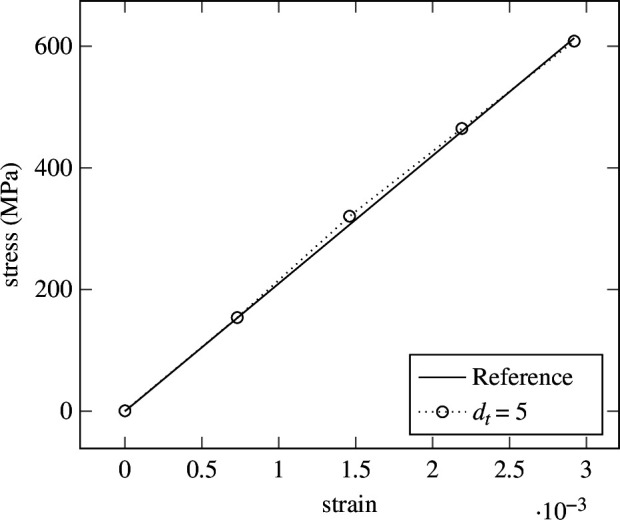
Elasticity—prediction in five strain (time) steps. Prediction of the LIF from equation (2.15) for ${\displaystyle d_t=5}$ . Deviations from the true solution can be observed in the middle part.

Figure 11.

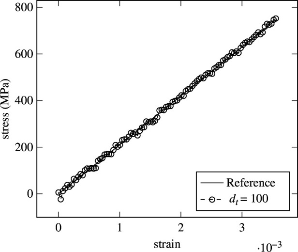
Elasticity—prediction in 100 strain (time) steps. Prediction of the LIF from equation (2.15) for ${\displaystyle d_t=100}$ . Fluctuations around the true solution can be observed.

Remark: The seemingly simple linear regression task provides a challenge for SNN, as effectively an ordinary differential equation has to be fitted to a linear function while relying on binary information transmission and inexact gradients.

3. Nonlinear regression using recurrent leaky integrate and fire

In order to counter the problems of vanishing information for a large number of strain (time) steps encountered in the preceding section, a recurrent SNN architecture is proposed (§3.1). Its performance is demonstrated by means of a numerical example in §3.2.

3.1. Recurrent leaky integrate and fire

The standard LIF is a feed-forward neuron, such that information is flowing unidirectionally in the form of spikes. By adding a feedback loop, a recurrent LIF (RLIF) can be formulated, which builds on the standard recurrent neural network (RNN) formulation. This enables the network to use relationships along several time steps for the prediction of the current time step. It was shown in Pascanu et al. [100] that recurrent loops can retain information for a relatively longer number of time steps when compared with their non-recurrent counterparts.

Here, the formulation of the hidden layer in equation (2.5) includes additional recurrent weights ${\displaystyle {\mathit{V}}_{\eta }^{(l)}}$ , such that

$${\displaystyle {\displaystyle h_{\eta ,t}^{(l)}={\varphi }^{(l)}\left({\mathit{W}}_{\eta }^{(l)}{\mathit{h}}_t^{(l-1)}+{\mathit{V}}_{\eta }^{(l)}{\mathit{h}}_{t-1}^{(l-1)}\right).}}$$ (3.1)

In this RNN, the influence of the preceding time step is explicitly included by means of additional recurrent weights ${\displaystyle {\mathit{V}}_{\eta }^{(l)}}$ . The resulting set of trainable parameters reads

$${\displaystyle {\displaystyle {\mathit{\theta }}_{\text{RNN}}=\left\{{\mathit{W}}_{\eta }^{(l)},{\mathit{V}}_{\eta }^{(l)}\right\}.}}$$ (3.2)

The RNN formulation can be included in the LIF formulation from equation (2.7) to obtain an RLIF, such that

$${\displaystyle {\displaystyle \begin{array}{rl}{U}_{\eta ,t}^{(l)}& ={\beta }_{\eta }^{(l)}{U}_{\eta ,t-1}^{(l)}+{\mathit{W}}_{\eta }^{(l)}{\mathit{h}}_t^{(l-1)}\\ & +{\mathit{V}}_{\eta }^{(l)}{\mathit{h}}_{t-1}^{(l-1)}-{\varphi }_{\text{spk},t-1}^{(l)}{U}_{\text{thr},\eta }^{(l)},\end{array}}}$$ (3.3)

where ${\displaystyle U_{\eta ,t}^{(l)}}$ is again the membrane potential of the ${\displaystyle \eta }$ th neural unit at time ${\displaystyle t}$ , ${\displaystyle U_{\text{thr},\eta }^{(l)}}$ denotes the membrane threshold, ${\displaystyle {\beta }_{\eta }^{(l)}}$ is the membrane potential decay rate and ${\displaystyle {\mathit{W}}_{\eta }^{(l)}{\mathit{h}}_t^{(l-1)}}$ is the standard ANN weight multiplied with the preceding layer at the current time step. Additionally, ${\displaystyle {\mathit{V}}_{\eta }^{(l)}}$ denotes the recurrent weights from equation (3.1). This leads to the following set of trainable parameters

$${\displaystyle {\displaystyle {\mathit{\theta }}_{\text{RLIF}}=\left\{{\mathit{W}}_{\eta }^{(l)},{\mathit{V}}_{\eta }^{(l)},{\beta }_{\eta }^{(l)},U_{\text{thr},\eta }^{(l)}\right\}.}}$$ (3.4)

3.2. Numerical experiment: Ramberg–Osgood

The performance of the RLIF is investigated in nonlinear function regression. As a first test case, the nonlinear Ramberg–Osgood power law for modelling history-independent plasticity is considered, in which stress ${\displaystyle \sigma }$ and strain ${\displaystyle \epsilon }$ are related via

$${\displaystyle {\displaystyle \epsilon =\frac{\sigma }{E}+0.002{\left(\frac{\sigma }{{\sigma }_Y}\right)}^n.}}$$ (3.5)

Here, ${\displaystyle \epsilon }$ is the infinitesimal, one-dimensional elastic strain, ${\displaystyle \sigma }$ denotes the one-dimensional Cauchy stress, ${\displaystyle E}$ is Young’s modulus, ${\displaystyle n}$ is a material constant describing the hardening behaviour of plastic deformation and ${\displaystyle {\sigma }_Y}$ is the yield strength of the material. Note that this plasticity model is only suited for a single loading direction and does not incorporate accumulation of plastic strain.

To this end, the general model described in §2.1 using RLIF defined in equation (3.3) is used. For a given strain history ${\displaystyle {\epsilon }_t}$ , the stress response for different values of yield stress ${\displaystyle {\sigma }_Y}$ is predicted with the following parametric architecture

$${\displaystyle {\displaystyle \begin{array}{rl}\mathcal{S}\left({\sigma }_Y\right)& ={\mathit{h}}_t^{\text{pop}}\circ {\mathit{h}}_t^{\text{dec}}\circ {\mathit{h}}_t^{\text{RLIF}}\circ {\mathit{h}}_t^{\text{RLIF}}\circ {\mathit{h}}_t^{\text{RLIF}}\\ & \circ {\mathit{h}}_t^{\text{const}}\left({\sigma }_Y\right)={\sigma }_t.\end{array}}}$$ (3.6)

The training data consists of yield strength ${\displaystyle {\sigma }_Y}$ as input for fixed strains in the interval ${\displaystyle \epsilon =[0,0.01]}$ for ${\displaystyle d_t=20}$ strain steps. The yield strength is uniformly sampled in the interval ${\displaystyle {\sigma }_Y=[100,500]}$ MPa, and the stress output is calculated according to equation (3.5). The Young’s modulus is chosen as ${\displaystyle E=2.1\times {10}^5}$ MPa and ${\displaystyle n=10}$ . Three datasets are generated, namely, training set, validation and test set with ${\displaystyle n_{\text{train}}=n_{\text{val}}=n_{\text{test}}=1024}$ samples, respectively. All three sets are standardized using the mean and standard deviation from the training set. The batch size is chosen as ${\displaystyle n_{\text{batch}}=1024}$ . The number of neurons ${\displaystyle n_u}$ is chosen as ${\displaystyle n_u=128}$ and is kept constant over all layers. The training is carried out for ${\displaystyle 5\times {10}^3}$ epochs. The model performing best on the validation set is chosen for subsequent evaluations. The mean relative error and the mean relative error of the last strain step with respect to the test set are reported.

In figure 12, different stress–strain curves are depicted for different yield strength values, obtained by solving equation (3.5) for the stress ${\displaystyle \sigma }$ with a classical Newton–Raphson method. The results of five different samples, randomly chosen from the ${\displaystyle n_{test}=1024}$ test samples, can be seen in figure 13. For the test set, a mean relative error for all strain steps of ${\displaystyle 8.7934\times {10}^{-2}}$ and a mean relative error for the last strain step of ${\displaystyle 8.0200\times {10}^{-2}}$ are obtained. The predictions on these five samples are more accurate than would be suspected from the mean relative error. The cause can be found in figure 14, where the mean relative error for all strain steps is plotted for every sample of the test set. It can be observed that a small number of samples has a much higher error than the rest, which impacts the error measure. This is caused by the purely data-driven nature of the experiment and can be tackled with approaches introduced in, for example, [101–103] .

Figure 12.

Ramberg–Osgood—reference solutions. Stress–strain curves of the Ramberg–Osgood material model for five different values of the yield stress ${\displaystyle {\sigma }_Y}$ obtained with Newton–Raphson algorithm.

Figure 13.

Ramberg–Osgood—RLIF prediction. Prediction of the RLIF from equation (3.6) for five different yield strength ${\displaystyle {\sigma }_Y}$ sampled from the test set for the nonlinear Ramberg–Osgood plasticity law.

Figure 14.

Ramberg–Osgood—RLIF test error. The mean relative error over all strain steps for 1024 samples from the test set for the numerical experiment is described in §3.2. It can be seen that some outliers have large error values, resulting in a mean error over all samples of ${\displaystyle 8.7934\times {10}^{-2}}$ . Most samples have a significantly lower error.

Nevertheless, the RLIF is able to regress on the varying yield strength ${\displaystyle {\sigma }_Y}$ and can predict the resulting nonlinear stress–strain behaviour, as can be seen in the predictions (figure 13). Deviations can be observed around the yield point as well as the endpoints of the curves. To be able to take into account long-term history-dependent behaviour, the RLIF formulation will be expanded towards the incorporation of explicit long-term memory in the next section, where a more complex plasticity model is investigated.

4. History-dependent regression using spiking long short-term memory network

To extend the limited memory of the RNN in §3, a SLSTM (§4.1) is proposed. Previously, SLSTM hs been considered for classification problems [71]. Herein, a novel regression approach with a population decoding layer is discussed by means of a history-dependent plasticity model (§4.2).

4.1. Spiking long short-term memory network

A SLSTM is the spiking version of the standard LSTM [104], where the latter is defined as

$${\displaystyle {\displaystyle h_{\eta ,t}^{(l)}=o_{\eta ,t}^{(l)}\odot {\varphi }_{\text{tanh}}\left(c_{\eta ,t}^{(l)}\right),}}$$ (4.1)

with

$${\displaystyle {\displaystyle \begin{array}{rl}{o}_{\eta ,t}^{(l)}& ={\varphi }_{\text{sigmoid}}\left({\mathit{W}}_{o,\eta }^{(l)}{\mathit{h}}_t^{(l-1)}+{\mathit{V}}_{o,\eta }^{(l)}{\mathit{h}}_{t-1}^{(l-1)}\right),\\ c_{\eta ,t}^{(l)}& =f_{\eta ,t}^{(l)}\odot c_{\eta ,t-1}^{(l)}+i_{\eta ,t}^{(l)}\odot {\tilde{c}}_{\eta ,t}^{(l)},\\ f_{\eta ,t}^{(l)}& ={\varphi }_{\text{sigmoid}}\left({\mathit{W}}_{f,\eta }^{(l)}{\mathit{h}}_t^{(l-1)}+{\mathit{V}}_{f,\eta }^{(l)}{\mathit{h}}_{t-1}^{(l-1)}\right),\\ i_{\eta ,t}^{(l)}& ={\varphi }_{\text{sigmoid}}\left({\mathit{W}}_{i,\eta }^{(l)}{\mathit{h}}_t^{(l-1)}+{\mathit{V}}_{i,\eta }^{(l)}{\mathit{h}}_{t-1}^{(l-1)}\right),\\ {\tilde{c}}_{\eta ,t}^{(l)}& ={\varphi }_{\text{tanh}}\left({\mathit{W}}_{c,\eta }^{(l)}{\mathit{h}}_t^{(l-1)}+{\mathit{V}}_{c,\eta }^{(l)}{\mathit{h}}_{t-1}^{(l-1)}\right),\end{array}}}$$

where ${\displaystyle f_t}$ denotes the forget gate with sigmoid activation ${\displaystyle {\varphi }_{\text{sigmoid}}}$ or tangent hyperbolicus activation ${\displaystyle {\varphi }_{\text{tanh}}}$ and corresponding weights ${\displaystyle {\mathit{W}}_f,{\mathit{V}}_f}$ with absorbed biases. The same nomenclature holds for the input gate ${\displaystyle i_t}$ , the output gate ${\displaystyle o_t}$ , the cell input ${\displaystyle {\tilde{c}}_t}$ and the cell state ${\displaystyle c_t}$ with their respective activations and weights. The new cell state ${\displaystyle c_t}$ and the output of the LSTM ${\displaystyle h_t}$ are formed using the Hadamard or point-wise product ${\displaystyle \odot }$ . The parameters of the LSTM are its weights, such that

$${\displaystyle {\displaystyle \begin{array}{rl}{\theta }_{\text{LSTM}}=\{& {\mathit{W}}_{f,\eta }^{(l)},{\mathit{W}}_{i,\eta }^{(l)},{\mathit{W}}_{o,\eta }^{(l)},{\mathit{W}}_{c,\eta }^{(l)},\\ & {\mathit{V}}_{f,\eta }^{(l)},{\mathit{V}}_{i,\eta }^{(l)},{\mathit{V}}_{o,\eta }^{(l)},{\mathit{V}}_{c,\eta }^{(l)}.\}.\end{array}}}$$ (4.2)

For detailed derivations and explanations of standard LSTM, see, for example, [85,86]. The SLSTM can be obtained from the LSTM by using spike activations within the LSTM formulation from equation (4.1) , such that

$${\displaystyle {\displaystyle h_{\eta ,t}^{(l)}=o_{\eta ,t}^{(l)}\odot {\varphi }_{\text{tanh}}\left(c_{\eta ,t}^{(l)}\right)-{\varphi }_{\text{spk},t-1}^{(l)}{U}_{\text{thr},\eta }^{(l)},}}$$ (4.3)

where the output ${\displaystyle h_{\eta ,t}^{(l)}}$ is used to determine if a spike is produced

$${\displaystyle {\displaystyle \begin{array}{r}{\varphi }_{\text{spk},t}^{(l)}=\{\begin{array}{l}1,h_{\eta ,t}^{(l)}\ge U_{\text{thr},\eta }^{(l)}\\ 0,h_{\eta ,t}^{(l)}<U_{\text{thr},\eta }^{(l)}.\end{array}\end{array}}}$$ (4.4)

In other words, the output of ${\displaystyle h_{\eta ,t}^{(l)}}$ can be interpreted as the membrane potential of the SLSTM, such that ${\displaystyle h_{\eta ,t}^{(l)}=U_{\eta ,t}^{(l)}}$ . A decay parameter ${\displaystyle \beta }$ is not used in this formulation. Rather than using decay to remove information from the cell state ${\displaystyle c_{\eta ,t}^{(l)}}$ , this is achieved by carefully regulated gates. The corresponding optimization parameters of the SLSTM are

$${\displaystyle {\displaystyle \begin{array}{rl}{\mathit{\theta }}_{\text{SLSTM}}=\{& {\mathit{W}}_{f,\eta }^{(l)},{\mathit{W}}_{i,\eta }^{(l)},{\mathit{W}}_{o,\eta }^{(l)},{\mathit{W}}_{c,\eta }^{(l)},\\ & {\mathit{V}}_{f,\eta }^{(l)},{\mathit{V}}_{i,\eta }^{(l)},{\mathit{V}}_{o,\eta }^{(l)},{\mathit{V}}_{c,\eta }^{(l)},U_{\text{thr},\eta }^{(l)}\}.\end{array}}}$$ (4.5)

Basically, the cell state ${\displaystyle c_{\eta ,t}^{(l)}}$ acts as long-term memory, just like in the standard LSTM formulation. The communication between layers is handled via spike trains that depend on the membrane potential ${\displaystyle h_{\eta ,t}^{(l)}=U_{\eta ,t}^{(l)}}$ in equation(4.3) and the activation function ${\displaystyle {\varphi }_{\text{spk},t}^{(l)}}$ from equation (4.4) .

4.2. Numerical experiment: Isotropic hardening using spiking long short-term memory network

The following numerical experiments aim to investigate the performance of the proposed SLSTM on nonlinear, history-dependent problems. Therefore, a one-dimensional plasticity model with isotropic hardening is investigated. Following Simo and Hughes [105], the model is defined by

$${\displaystyle {\displaystyle \begin{array}{rl}& 1.\epsilon ={\epsilon }_{\text{el}}+{\epsilon }_{\text{pl}},\\ & 2.\sigma =E\left(\epsilon -{\epsilon }_{\text{pl}}\right),\\ & 3.{\dot{\epsilon }}_{\text{pl}}=\gamma \mathrm{sign}\left(\sigma \right),\dot{\alpha }=\gamma ,\\ & 4.f\left(\sigma ,\alpha \right)=|\sigma |-\left({\sigma }_Y+K\alpha \right)\le 0,\\ & 5.\gamma \ge 0,f\left(\sigma ,\alpha \right)\le 0,\gamma f\left(\sigma ,\alpha \right)=0,\\ & 6.\gamma \dot{f}\left(\sigma ,\alpha \right)=0,\text{if}f\left(\sigma ,\alpha \right)=0,\end{array}}}$$ (4.6)

where

1. is the additive elastoplastic split of the small-strain tensor ${\displaystyle \epsilon }$ into a purely elastic part ${\displaystyle {\epsilon }_{\text{el}}}$ and a purely plastic part ${\displaystyle {\epsilon }_{\text{el}}}$ ;

2. denotes the elastic stress–strain relationship for the Cauchy stress tensor ${\displaystyle \sigma }$ and elastic modulus ${\displaystyle E}$ ;

3. describes the flow rule and isotropic hardening law with consistency parameter ${\displaystyle \gamma }$ and equivalent plastic strain ${\displaystyle \alpha }$ ;

4. gives the yield condition ${\displaystyle f\left(\sigma ,\alpha \right)}$ with hardening modulus ${\displaystyle K}$ ;

5. denotes the Kuhn–Tucker complementarity conditions; and

6. describes the consistency condition.

In figure 15, different stress–strain paths are shown for varying strains. Especially long-time dependencies are of interest. To this end, the predictive capabilities of the SNN are investigated for inference over ${\displaystyle d_t=100}$ strain steps, where the elastoplastic model is evaluated using a classical explicit return-mapping algorithm, see Simo and Hughes [105].

Figure 15.

Isotropic hardening—reference solutions. Five stress–strain curves sampled from the isotropic hardening material model for different maximum strains obtained from equation (4.6).

The training data consists of strain as input, uniformly sampled in the interval ${\displaystyle \epsilon =[0,0.01]}$ , and stress as output calculated according to equation (4.6). The yield stress is chosen as ${\displaystyle {\sigma }_Y=300}$ MPa, the elastic modulus ${\displaystyle E=2.1\times {10}^5}$ MPa and the hardening modulus as ${\displaystyle 2.1\times {10}^4}$ MPa. Three datasets are generated, namely, a training set with ${\displaystyle n_{\text{train}}=10240}$ samples and a validation set and test set with ${\displaystyle n_{\text{val}}=n_{\text{test}}=1024}$ samples. All three sets are standardized using the mean and standard deviation from the training set. The batch size is chosen as ${\displaystyle n_{\text{batch}}=1024}$ . The training is carried out for 500 epochs. The model performing best on the validation set is chosen for subsequent evaluations. The mean relative error accumulated over all time steps and the mean relative error of the last strain step with respect to the test set are reported.

4.2.1. Influence of hyperparameter

The first study investigates the prediction accuracy as a function of (i) the number of output neurons, which participate in the population regression outlined in §2.1 and (ii) different capacities of the SLSTM in the sense of layer width. To this end, the SLSTM defined in equation (4.3) is used, resulting in the following architecture:

$${\displaystyle {\displaystyle \begin{array}{rl}{\mathcal{S}}_{\mathit{\text{SLSTM}}}\left({\epsilon }_t\right)& ={\mathit{h}}_t^{\text{pop}}\circ {\mathit{h}}_t^{\text{dec}}\circ {\mathit{h}}_t^{\text{SLSTM}}\circ {\mathit{h}}_t^{\text{SLSTM}}\circ {\mathit{h}}_t^{\text{SLSTM}}\\ & \circ {\mathit{h}}_t^{\text{const}}\left({\epsilon }_t\right)={\sigma }_t.\end{array}}}$$ (4.7)

Multiple simulations with output neurons and hidden layers drawn from the grid ${\displaystyle n_u\times n_o=[16,32,64,128,256]\times [16,32,64,128,256]}$ are carried out. The resulting mean relative error for all strain steps with respect to the test set is shown in figure 16, whereas the resulting mean relative error of the last strain step with respect to the test set is depicted in figure 17. A clear convergence behaviour can be observed for the number of hidden neurons ${\displaystyle n_u}$ , where larger numbers of neurons lead to lower errors. For the number of output neurons ${\displaystyle n_o}$ , a tendency can be observed upon convergence with respect to ${\displaystyle n_u}$ . For the largest number of hidden neurons ${\displaystyle n_u=256}$ , the mean relative error over all strain steps and the mean relative error of the last strain step get larger for ${\displaystyle n_o=[128,256]}$ output neurons, whereas for ${\displaystyle n_o=[16,32,64]}$ the errors are almost the same. The lowest mean relative error for all strain steps is ${\displaystyle 5.2445\times {10}^{-2}}$ for ${\displaystyle n_u=256}$ hidden neurons per layer and ${\displaystyle n_o=64}$ output neurons. The lowest mean relative error for the last strain steps is ${\displaystyle 2.8729\times {10}^{-3}}{\displaystyle n_u=256}$ hidden neurons per layer and ${\displaystyle n_o=32}$ output neurons. Again, the seemingly high errors are caused by outliers polluting the average, as also observed in §3.2. The same counter-measures discussed in §3.2 can be applied to prohibit outliers, for example, by enforcing thermodynamic consistency.

Figure 16.

Isotropic hardening—error versus width. The mean relative error of the last strain step versus the number of hidden neurons per layer is shown for different numbers of output neurons in the isotropic hardening experiment from §4 using the SLSTM from equation (4.7).

Figure 17.

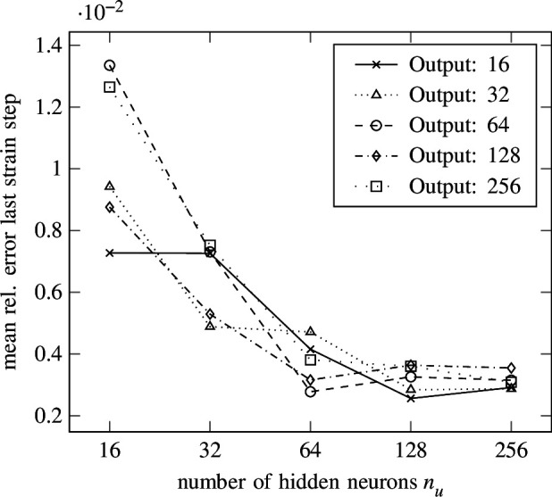
Isotropic hardening—error versus width. The mean relative error of all strain steps versus the number of hidden neurons per layer is shown for different numbers of output neurons in the isotropic hardening experiment from §4 using the SLSTM from equation (4.7) .

4.2.2. Energy and memory efficiency

For the second experiment, the SLSTM using ${\displaystyle n_o=64}$ output neurons and ${\displaystyle n_u=256}$ hidden neurons per layer are compared with a standard LSTM with an equal number of optimization parameters. The aim of this study is the comparison of the prediction accuracy, but also the difference in memory and energy consumption on neuromorphic hardware. For both ANN variants to be comparable, the same topology is chosen for the LSTM as for the SLSTM, such that

$${\displaystyle {\displaystyle \begin{array}{rl}{\mathcal{N}}_{\mathit{\text{LSTM}}}\left({\epsilon }_t\right)& ={\mathit{h}}_t^{\text{dense}}\circ {\mathit{h}}_t^{\text{dense}}\circ {\mathit{h}}_t^{\text{LSTM}}\circ {\mathit{h}}_t^{\text{LSTM}}\circ {\mathit{h}}_t^{\text{LSTM}}\\ & \circ {\mathit{h}}_t^{\text{const}}\left({\epsilon }_t\right)={\sigma }_t,\end{array}}}$$ (4.8)

where the last two layers are replaced by densely connected conventional feed-forward neural networks. Again, the training was carried out for ${\displaystyle 5\times {10}^3}$ epochs and the same datasets from the previous experiments are used. The standard LSTM from equation (4.8) reached a mean relative error of ${\displaystyle 4.8611\times {10}^{-2}}$ over all strain steps and a mean relative error of ${\displaystyle 4.7569\times {10}^{-3}}$ for the last strain step. The SLSTM from equation (4.7) reached a mean relative error of ${\displaystyle 9.3832\times {10}^{-2}}$ over all strain steps and a mean relative error of ${\displaystyle 4.0497\times {10}^{-3}}$ for the last strain step. The resulting prediction for one strain path is illustrated in figure 18. Clearly, both networks are able to accurately predict the history-dependent, nonlinear stress–strain behaviour.

Figure 18.

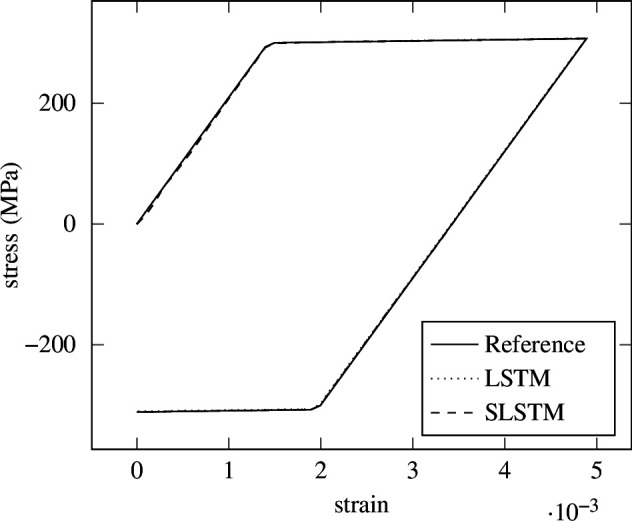
Isotropic hardening—LSTM versus SLSTM. Prediction of a single load path using the return-mapping algorithm as a reference, the standard LSTM and the spiking LSTM formulation.

Some deviations from the SLSTM can be seen at the beginning of the curve. The dynamics of the spiking formulation result in a higher mean relative error over all strain steps with respect to the LSTM. However, the endpoint has a better fit than the LSTM. This is seen in the lower error at the last strain step.

To assess the potential of interfacing our model in embedded, resource-constrained sensors in the wild, we performed a series of power profiling experiments for our SNNs (both using LIF neurons and SLSTMs) when processed on the Loihi neuromorphic chip [54]. These results are compared against their non-spiking equivalents on an NVIDIA V100 GPU. Data were extracted using the energy profiler in KerasSpiking v. 0.3.0. The emulation tool takes all non-zero activations, accumulates the operation count of each activation (i.e. the fan-out of the activated neuron) and scales this by the estimated energy cost per operation. Specifically, this operation is a ‘read-and-accumulate’, where the presence of a spike requires all connected synapses to be ‘read’ from memory and accumulated with other terms. Other literature refers to this as ‘SynOps’ or ‘Synaptic Operations’ [106–110]. This is a coarse, but reasonable, approximation for small-scale models as neuromorphic hardware skips processing non-zero activations. For large-scale models that require inter-chip data communication, the energy cost of overhead is not accounted for in such a model. For our purposes, with lightweight, low-power models, this is an acceptable approximation. It is also the de facto metric for measuring energy efficiency in silico from the NeuroBench [110] initiative, which aims to find representative benchmarking of neuromorphic models.

The first difference in energy usage is that the spiking implementation is measured in an ‘event-based’ manner, where processing only occurs when a neuron emits a spike. In contrast, a non-spiking network processed on a GPU continuously computes with all activations. The second difference is that SNNs require multiple strain steps of a forward pass, whereas their non-spiking counterparts do not (unless the input to the network varies over time). Note that the cost of overhead did not need to be accounted for (i.e. transferring data between devices) because all models fit on a single device.

Each network has been broken up into its constituent layers to measure how much they contribute to energy usage on each device. The total energy consumption per forward pass of the non-spiking network on the V100 is 512 nJ, whereas the equivalent SNN is 4.25 nJ. This represents a 120× reduction in energy consumption. The non-spiking LSTM network consumed 5.7 µJ while the proposed SLSTM architecture required 24 nJ, a 238× reduction. Detailed results are summarized in table 1.

Table 1.

Comparison between spiking and non-spiking forward-pass energy consumption and memory usage.

architecture	energy		architecture	energy
dense	Loihi (nJ)	GPU (nJ)	LSTM	Loihi (nJ)	GPU (nJ)
FC1	6.9e-2	0.61	LSTM1	0.28	2.5
FC2	1.3	160	LSTM2	11	2.5e3
FC3	1.3	160	LSTM3	10	2.5e3
FC4	1.2	160	FC1	2.6	630
FC5	0.3	39	FC2	0.21	39
total energy	4.25	512	total energy	24	5.7e3
reduction	×120		reduction factor	×238
synaptic memory	0.86 MB		synaptic memory	9.5 MB

5. Conclusion and outlook

In the present study, a framework for regression using SNNs was proposed based on a membrane potential spiking decoder and a population voting layer. Several numerical examples using different spiking neural architectures investigated the performance of the introduced topology towards linear, nonlinear and history-dependent regression problems.

First, a simple feed-forward SNN, the LIF, was derived from the classical densely connected feed-forward ANN. It was shown that the SNN can be seen as a special kind of activation function, which produces binary outputs, so-called spikes. These spikes are used to propagate information through a possibly deep SNN. The spikes occur due to the dynamic behaviour of the membrane potential inside the neuron, which rises when spikes appear at the input and decays over time if no spikes appear. If a certain threshold value is reached, the membrane potential is reset and the neuron emits a spike itself. This formulation introduces more hyperparameters, which fortunately can be learned during training. The spikes introduce sparsity in the network, which can be effectively exploited by neuromorphic hardware to improve latency, power and memory efficiency. The non-differentiability of the binary spikes is circumvented by surrogate gradients during backpropagation.

Next, a network topology was proposed, which decodes binary spikes into real numbers, which is essential for all kinds of regression problems. A decoding layer takes the membrane potentials of all neurons in the last spiking layer and propagates them to a population voting layer, which provides its mean potential resulting in a real number. The proposed topology can be used for arbitrary temporal input and output dimensions. A simple experiment on a linear elastic material model using LIFs showed that the proposed topology is able to regress the problem. It was shown that errors are introduced for a large number of strain steps. This problem was overcome by introducing RLIF, which extends the LIF by recurrent feedback loops. An experiment using a nonlinear Ramberg–Osgood plasticity model showed that the proposed topology using RLIF is able to regress varying yield limits accurately. The final extension was concerned with the introduction of explicit long-term memories inspired by the classical LSTM formulation, resulting in a spiking LSTM. The performance of this SLSTM was investigated on a history-dependent isotropic hardening model, where different load paths were accurately regressed. During prediction, the SLSTM was able to generalize even better than the LSTM for the final load step. Furthermore, the convergence of the proposed method was shown. Note that an extension towards two- and three-dimensional mechanical problems is equally possible. This will involve learning a functional relationship for each stress component, which can be either achieved by a multi-input/output architecture or by using individual networks for each stress component. This treatment is analogous to second-generation ANN, see for instance [111], where stress data has been decoupled using Proper orthogonal decomposition (POD).

Power profiling and memory analysis were conducted on the LIF and SLSTM networks to compare efficiency on neuromorphic hardware as against a GPU. The Loihi neuromorphic processor was able to achieve a 120× reduction in energy consumption when processing the dense LIF network, and the SLSTM offered a 238× reduction in energy during inference.

The range of possible future application scenarios enabled by regression with SNN are manifold. For instance, today’s sensing systems cannot capture all quantities that are relevant for structural health monitoring. In the context of mechanics, displacement and strain are quite easy to assess, but the mechanical stress, which reflects the actual response of structures and materials to deformation, remains a so-called hidden quantity. Physics-informed machine learning offers the potential to reconstruct hidden quantities from data by leveraging information from physical models, given in the form of partial differential equations. It is expected that the developments in the field of neuromorphic hardware will foster the development of a new generation of embedded systems, which will ultimately enable control of structures and processes based on partial differential equations.

Ethics

This work did not require ethical approval from a human subject or animal welfare committee.

Data accessibility

The code is available at: https://github.com/ahenkes1/HENKES_SNN and Zenodo [112].

Declaration of AI use

We have not used AI-assisted technologies in creating this article.

Authors’ contributions

A.H.: conceptualization, data curation, formal analysis, funding acquisition, investigation, methodology, project administration, resources, software, supervision, validation, visualization, writing—original draft, writing—review and editing; J.K.E.: conceptualization, funding acquisition, software, supervision, writing—original draft, writing—review and editing; H.W.: conceptualization, funding acquisition, resources, supervision, visualization, writing—review and editing.

All authors gave final approval for publication and agreed to be held accountable for the work performed therein.

Conflict of interest declaration

The authors declare that they have no known competing financial interests or personal relationships that could have appeared to influence the work reported in this paper.

Funding

No funding has been received for this article.

References

- 1. Hornik K, Stinchcombe M, White H. 1989. Multilayer feedforward networks are universal approximators. Neural Netw. 2 , 359–366. ( 10.1016/0893-6080(89)90020-8) [DOI] [Google Scholar]
- 2. Cybenko G. 1989. Approximation by superpositions of a sigmoidal function. Math. Control. Signal. Syst. 2 , 303–314. ( 10.1007/BF02551274) [DOI] [Google Scholar]
- 3. Chen T, Chen H. 1995. Universal approximation to nonlinear operators by neural networks with arbitrary activation functions and its application to dynamical systems. IEEE Trans. Neural Netw. 6 , 911–917. ( 10.1109/72.392253) [DOI] [PubMed] [Google Scholar]
- 4. Julius B, Philipp G, Gitta K, Philipp P. 2021. The modern mathematics of deep learning. arXiv. See https://arxiv.org/abs/2105.04026
- 5. Kutz JN. 2017. Deep learning in fluid dynamics. J. Fluid Mech. 814 , 1–4. ( 10.1017/jfm.2016.803) [DOI] [Google Scholar]
- 6. Wei-Wei Z, Bernd RN. 2021. Artificial intelligence in fluid mechanics. Acta Mech. Sin. 37 , 1715–1717. ( 10.1007/s10409-021-01154-3) [DOI] [Google Scholar]
- 7. Cai S, Mao Z, Wang Z, Yin M, Karniadakis GE. 2021. Physics-informed neural networks (PINNs) for fluid mechanics: a review. Acta Mech. Sin. 37 , 1–12. ( 10.1007/s10409-021-01148-1) [DOI] [Google Scholar]
- 8. Raissi M, Yazdani A, Karniadakis GE. 2020. Hidden fluid mechanics: learning velocity and pressure fields from flow visualizations. Science 367 , 1026–1030. ( 10.1126/science.aaw4741) [DOI] [PMC free article] [PubMed] [Google Scholar]
- 9. Henning W, Christian W, Peter W. 2020. The neural particle method – an updated Lagrangian physics informed neural network for computational fluid dynamics. Comput. Methods Appl. Mech. Eng. 368 , 113127. ( 10.1016/j.cma.2020.113127) [DOI] [Google Scholar]
- 10. Haghighat E, Raissi M, Moure A, Gomez H, Juanes R. 2021. A physics-informed deep learning framework for inversion and surrogate modeling in solid mechanics. Comput. Methods Appl. Mech. Eng. 379 , 113741. ( 10.1016/j.cma.2021.113741) [DOI] [Google Scholar]
- 11. Buffa G, Fratini L, Micari F. 2012. Mechanical and microstructural properties prediction by artificial neural networks in FSW processes of dual phase titanium alloys. J. Manuf. Process. 14 , 289–296. ( 10.1016/j.jmapro.2011.10.007) [DOI] [Google Scholar]
- 12. Abueidda DW, Lu Q, Koric S. 2021. Meshless physics‐informed deep learning method for three‐dimensional solid mechanics. Numer. Meth. Eng. 122 , 7182–7201. ( 10.1002/nme.6828) [DOI] [Google Scholar]
- 13. Nie Z, Jiang H, Kara LB. 2020. Stress field prediction in cantilevered structures using convolutional neural networks. J. Comput. Inf. Sci. Eng. 20 , 011002. ( 10.1115/1.4044097) [DOI] [Google Scholar]
- 14. Henkes A, Caylak I, Mahnken R. 2021. A deep learning driven pseudospectral PCE based FFT homogenization algorithm for complex microstructures. Comput. Methods Appl. Mech. Eng. 385 , 114070. ( 10.1016/j.cma.2021.114070) [DOI] [Google Scholar]
- 15. Henkes A, Wessels H, Mahnken R. 2022. Physics informed neural networks for continuum micromechanics. Comput. Methods Appl. Mech. Eng. 393 , 114790. ( 10.1016/j.cma.2022.114790) [DOI] [Google Scholar]
- 16. Mianroodi JR, H. Siboni N, Raabe D. Teaching solid mechanics to artificial intelligence—a fast solver for heterogeneous materials. Npj Comput. Mater. 7 , 99. ( 10.1038/s41524-021-00571-z) [DOI] [Google Scholar]
- 17. Méndez-Mancilla A, Wessels HH, Legut M, Kadina A, Mabuchi M, Walker J, Robb GB, Holden K, Sanjana NE. 2022. Chemically modified guide Rnas enhance CRISPR-Cas13 knockdown in human cells. In Current trends and open problems in computational mechanics, pp. 569–579. Springer. See https://www.sciencedirect.com/science/article/pii/S2451945621003512. [DOI] [PMC free article] [PubMed] [Google Scholar]
- 18. Dehghani H, Zilian A. 2020. Poroelastic model parameter identification using artificial neural networks: on the effects of heterogeneous porosity and solid matrix Poisson ratio. Comput. Mech. 66 , 625–649. ( 10.1007/s00466-020-01868-4) [DOI] [Google Scholar]
- 19. Thakolkaran P, Joshi A, Zheng Y, Flaschel M, De Lorenzis L, Kumar S. 2022. NN-EUCLID: Deep-learning hyperelasticity without stress data. arXiv 169 , 105076. (https://arxiv.org/abs/2205.06664) [Google Scholar]
- 20. Zhang E, Yin M, Karniadakis GE. 2020. Physics-informed neural networks for nonhomogeneous material identification in elasticity imaging. arXiv. See https://arxiv.org/abs/2009.04525
- 21. Zhang E, Dao M, Karniadakis GE, Suresh S. 2022. Analyses of internal structures and defects in materials using physics-informed neural networks. Sci. Adv. 8 , eabk0644. ( 10.1126/sciadv.abk0644) [DOI] [PMC free article] [PubMed] [Google Scholar]
- 22. Anton D, Wessels H. 2022. Physics-informed neural networks for material model calibration from full-field displacement data. arXiv. See https://arxiv.org/abs/2212.07723
- 23. As’ad F, Avery P, Farhat C. 2022. A mechanics‐informed artificial neural network approach in data‐driven constitutive modeling. J. Numer. Meth. Eng. 123 , 2738–2759. ( 10.1002/nme.6957) [DOI] [Google Scholar]
- 24. Yang H, Qiu H, Xiang Q, Tang S, Guo X. 2020. Exploring elastoplastic constitutive law of microstructured materials through artificial neural network—a mechanistic-based data-driven approach. J. Appl. Mech. 87 , 091005. ( 10.1115/1.4047208) [DOI] [Google Scholar]
- 25. Xu K, Huang DZ, Darve E. 2021. Learning constitutive relations using symmetric positive definite neural networks. J. Comput. Phys. 428 , 110072. ( 10.1016/j.jcp.2020.110072) [DOI] [Google Scholar]
- 26. Fernández M, Rezaei S, Rezaei Mianroodi J, Fritzen F, Reese S. 2020. Application of artificial neural networks for the prediction of interface mechanics: a study on grain boundary constitutive behavior. Adv. Model. Simul. in Eng. Sci. 7 , 1–27. ( 10.1186/s40323-019-0138-7) [DOI] [Google Scholar]
- 27. Aldakheel F, Satari R, Wriggers P. 2021. Feed-forward neural networks for failure mechanics problems. Appl. Sci. 11 , 6483. ( 10.3390/app11146483) [DOI] [Google Scholar]
- 28. Liu SW, Huang JH, Sung JC, Lee CC. 2002. Detection of cracks using neural networks and computational mechanics. Comput. Methods Appl. Mech. Eng. 191 , 2831–2845. ( 10.1016/S0045-7825(02)00221-9) [DOI] [Google Scholar]
- 29. Henkes A, Wessels H. 2022. Three-dimensional microstructure generation using generative adversarial neural networks in the context of continuum micromechanics. arXiv. See https://arxiv.org/abs/2206.01693
- 30. Hsu T, Epting WK, Kim H, Abernathy HW, Hackett GA, Rollett AD, Salvador PA, Holm EA. 2021. Microstructure generation via generative adversarial network for heterogeneous, topologically complex 3D materials. JOM 73 , 90–102. ( 10.1007/s11837-020-04484-y) [DOI] [Google Scholar]
- 31. Mosser L, Dubrule O, Blunt MJ. 2017. Reconstruction of three-dimensional porous media using generative adversarial neural networks. Phys. Rev. E 96 , 043309. ( 10.1103/PhysRevE.96.043309) [DOI] [PubMed] [Google Scholar]
- 32. Ma J, Dong S, Chen G, Peng P, Qian L. 2021. A data-driven normal contact force model based on artificial neural network for complex contacting surfaces. Mech. Syst. Signal Process. 156 , 107612. ( 10.1016/j.ymssp.2021.107612) [DOI] [Google Scholar]
- 33. Öner E, Şengül Şabano B, Uzun Yaylacı E, Adıyaman G, Yaylacı M, Birinci A. 2022. On the plane receding contact between two functionally graded layers using computational, finite element and artificial neural network methods. Z. Angew. Math. Mech. 102 , e202100287. ( 10.1002/zamm.202100287) [DOI] [Google Scholar]
- 34. Ardestani MM, Chen Z, Wang L, Lian Q, Liu Y, He J, Li D, Jin Z. 2014. Feed forward artificial neural network to predict contact force at medial knee joint: application to gait modification. Neurocomputing 139 , 114–129. ( 10.1016/j.neucom.2014.02.054) [DOI] [Google Scholar]
- 35. Feng Z, Yan J, Gao Y. 2022. Prediction of contact resistance between copper blocks under cyclic load based on deep learning algorithm. AIP Adv. 12 , 075009. ( 10.1063/5.0095871) [DOI] [Google Scholar]
- 36. Cai S, Wang Z, Wang S, Perdikaris P, Karniadakis GE. 2021. Physics-informed neural networks for heat transfer problems. J. Heat Transfer. 143 , 6. ( 10.1115/1.4050542) [DOI] [Google Scholar]
- 37. Laubscher R. 2021. Simulation of multi-species flow and heat transfer using physics-informed neural networks. Phys. Fluids 33 . ( 10.1063/5.0058529) [DOI] [Google Scholar]
- 38. Tamaddon-Jahromi HR, Chakshu NK, Sazonov I, Evans LM, Thomas H, Nithiarasu P. 2020. Data-driven inverse modelling through neural network (deep learning) and computational heat transfer. Comput. Methods Appl. Mech. Eng. 369 , 113217. ( 10.1016/j.cma.2020.113217) [DOI] [Google Scholar]
- 39. Niaki SA, Haghighat E, Campbell T, Poursartip A, Vaziri R. 2021. Physics-informed neural network for modelling the thermochemical curing process of composite-tool systems during manufacture. Comput. Methods Appl. Mech. Eng. 384 , 113959. ( 10.1016/j.cma.2021.113959) [DOI] [Google Scholar]
- 40. Ramudo VAF. 2020. Machine learning to build reduced order models of solid mechanic models with uncertainty. Master’s thesis, Universitat Politècnica de Catalunya. [Google Scholar]
- 41. Balokas G, Czichon S, Rolfes R. 2018. Neural network assisted multiscale analysis for the elastic properties prediction of 3D braided composites under uncertainty. Compos. Struct. 183 , 550–562. ( 10.1016/j.compstruct.2017.06.037) [DOI] [Google Scholar]
- 42. Fuhg JN, Kalogeris I, Fau A, Bouklas N. 2022. Interval and fuzzy physics-informed neural networks for uncertain fields. Probabilistic Eng. Mech. 68 , 103240. ( 10.1016/j.probengmech.2022.103240) [DOI] [Google Scholar]
- 43. Olivier A, Shields MD, Graham-Brady L. 2021. Bayesian neural networks for uncertainty quantification in data-driven materials modeling. Comput. Methods Appl. Mech. Eng. 386 , 114079. ( 10.1016/j.cma.2021.114079) [DOI] [Google Scholar]
- 44. Bock FE, Aydin RC, Cyron CJ, Huber N, Kalidindi SR, Klusemann B. 2019. A review of the application of machine learning and data mining approaches in continuum materials mechanics. Front. Mater. 6 , 110. ( 10.3389/fmats.2019.00110) [DOI] [Google Scholar]
- 45. Kumar S, Kochmann DM. 2021. What machine learning can do for computational solid mechanics. In Current trends and open problems in computational mechanics (eds Aldakheel F, Hudobivnik B, Soleimani M, Wessels H, Weißenfels C, Marino M), pp. 275–285. Cham: Springer. See https://link.springer.com/chapter/10.1007/978-3-030-87312-7_27. ( 10.1007/978-3-030-87312-7_27) [DOI] [Google Scholar]
- 46. Blechschmidt J, Ernst OG. 2021. Three ways to solve partial differential equations with neural networks — A review. GAMM-Mitteilungen 44 , e202100006. ( 10.1002/gamm.202100006) [DOI] [Google Scholar]
- 47. Roy K, Jaiswal A, Panda P. 2019. Towards spike-based machine intelligence with neuromorphic computing. Nature 575 , 607–617. ( 10.1038/s41586-019-1677-2) [DOI] [PubMed] [Google Scholar]
- 48. Indiveri G, Liu SC. 2015. Memory and Information Processing in Neuromorphic Systems. Proc. IEEE 103 , 1379–1397. ( 10.1109/JPROC.2015.2444094) [DOI] [Google Scholar]
- 49. Burr GW, et al. 2017. Neuromorphic computing using non-volatile memory. Adv. Phys.-X 2 , 89–124. ( 10.1080/23746149.2016.1259585) [DOI] [Google Scholar]
- 50. Narouie VB, Wessels H, Römer U. 2023. Inferring displacement fields from sparse measurements using the statistical finite element method. Mech. Syst. Signal Process 200 , 110574. ( 10.1016/j.ymssp.2023.110574) [DOI] [Google Scholar]
- 51. Perez-Nieves N, Goodman D. 2021. Sparse Spiking gradient descent. Adv. Neural Inf. Process. Syst 34 , 1795–11808. ( 10.1016/j.ymssp.2023.110574) [DOI] [Google Scholar]
- 52. Olshausen BA, Field DJ. 2006. What is the other 85 percent of V1 doing. In 23 problems in systems neuroscience (eds van Hemmen L, Sejnowski T), pp. 182–211, vol. 23 . See https://global.oup.com/academic/product/23-problems-in-systems-neuroscience-9780195148220?cc=ch&lang=en&;. ( 10.1093/acprof:oso/9780195148220.001.0001) [DOI] [Google Scholar]
- 53. Gerstner W, Kistler WM. 2002. Spiking neuron models: single neurons, populations, plasticity. Cambridge, UK: Cambridge University Press. ( 10.1017/CBO9780511815706) [DOI] [Google Scholar]
- 54. Davies M, et al. 2018. Loihi: a neuromorphic manycore processor with on-chip learning. IEEE Micro 38 , 82–99. ( 10.1109/MM.2018.112130359) [DOI] [Google Scholar]
- 55. Furber SB, Galluppi F, Temple S, Plana LA. 2014. The SpiNNaker project. Proc. IEEE 102 , 652–665. ( 10.1109/JPROC.2014.2304638) [DOI] [Google Scholar]
- 56. Merolla PA, et al. 2014. Artificial brains: a million spiking-neuron integrated circuit with a scalable communication network and interface. Science 345 , 668–673. ( 10.1126/science.1254642) [DOI] [PubMed] [Google Scholar]
- 57. Azghadi MR, Lammie C, Eshraghian JK, Payvand M, Donati E, Linares-Barranco B, Indiveri G. 2020. Hardware implementation of deep network accelerators towards healthcare and biomedical applications. IEEE Trans. Biomed. Circuits Syst. 14 , 1138–1159. ( 10.1109/TBCAS.2020.3036081) [DOI] [PubMed] [Google Scholar]
- 58. Frenkel C, Indiveri G. 2022. ReckOn: a 28nm sub-mm2 task-agnostic spiking recurrent neural network processor enabling on-chip learning over second-long timescales. In 2022 IEEE International Solid- State Circuits Conference (ISSCC). vol. 65. pp. 1–3 IEEE. [Google Scholar]
- 59. Ceolini E, Frenkel C, Shrestha SB, Taverni G, Khacef L, Payvand M, Donati E. 2020. Hand-gesture recognition based on EMG and event-based camera sensor fusion: a benchmark in neuromorphic computing. Front. Neurosci. 14 , 637. ( 10.3389/fnins.2020.00637) [DOI] [PMC free article] [PubMed] [Google Scholar]
- 60. Orchard G, Frady EP, Rubin DBD, Sanborn S, Shrestha SB, Sommer FT, Davies M. 2021. Efficient Neuromorphic signal processing with Loihi 2. In 2021 IEEE Workshop on Signal Processing Systems (SiPS) pp. 254–259, IEEE. [Google Scholar]
- 61. Yang S, Tan J, Chen B. 2022. Robust spike-based continual meta-learning improved by restricted minimum error entropy criterion. Entropy 24 , 455. ( 10.3390/e24040455) [DOI] [PMC free article] [PubMed] [Google Scholar]
- 62. Yang S, Chen B. 2023. Effective surrogate gradient learning with high-order information bottleneck for spike-based machine intelligence. IEEE Trans. Neural Netw. Learn. Syst. 1–15. ( 10.1109/TNNLS.2023.3329525) [DOI] [PubMed] [Google Scholar]
- 63. Yang S, Wang H, Chen B. 2023. SIBoLS: robust and energy-efficient learning for spike based machine intelligence in information bottleneck framework. IEEE Trans. Cogn. Dev. Syst. 1–13. ( 10.1109/TCDS.2023.3329532) [DOI] [Google Scholar]
- 64. Yang S, Chen B. 2023. Snib: Improving spike-based machine learning using nonlinear information bottleneck. IEEE Trans. Syst. Man Cybern. Syst. 53 , 7852–7863. ( 10.1109/TSMC.2023.3300318) [DOI] [Google Scholar]
- 65. Abadi M, et al. 2015. TensorFlow: large-scale machine learning on heterogeneous systems. See https://www.tensorflow.org/
- 66. Paszke A, et al. 2019. Pytorch: an imperative style, high-performance deep learning library. In Advances in neural information processing systems 32 (eds Wallach H, Larochelle H, Beygelzimer A, d’Alché-Buc F, Fox E, Garnett R), pp. 8024–8035. Curran Associates, Inc. See https://proceedings.neurips.cc/paper/2019/hash/bdbca288fee7f92f2bfa9f7012727740-Abstract.html. [Google Scholar]
- 67. Eshraghian JK, Ward M, Neftci E, Wang X, Lenz G, Dwivedi G, Bennamoun M, Jeong DS, Lu WD. 2021. Training spiking neural networks using lessons from deep learning. arXiv. See https://arxiv.org/abs/2109.12894
- 68. Fang W, Yu Z, Chen Y, Huang T, Masquelier T, Tian Y. 2021. Deep residual learning in spiking neural networks. Adv. Neural Inf. Process. Syst. 34 , 21. ( 10.48550/arXiv.2102.04159) [DOI] [Google Scholar]
- 69. Bellec G, Salaj D, Subramoney A, Legenstein R, Maass W. 2018. Long short-term memory and learning-to-learn in networks of spiking neurons. Adv. Neural Inf. Process. Syst. 31 . ( 10.48550/arXiv.1803.09574) [DOI] [Google Scholar]
- 70. Rao A, Plank P, Wild A, Maass W. 2022. A long short-term memory for AI applications in spike-based neuromorphic hardware. Nat. Mach. Intell. 4 , 467–479. ( 10.1038/s42256-022-00480-w) [DOI] [Google Scholar]
- 71. Yang Y, Eshraghian J, Truong ND, Nikpour A, Kavehei O. 2022. Neuromorphic deep spiking neural networks for seizure detection. See https://www.techrxiv.org/
- 72. Patel K, Hunsberger E, Batir S, Eliasmith C. 2021. A spiking neural network for image segmentation. arXiv. See https://arxiv.org/abs/2106.08921
- 73. Barchid S, Mennesson J, Eshraghian J, Djéraba C, Bennamoun M. 2023. Spiking neural networks for frame-based and event-based single object localization. arXiv. See https://arxiv.org/abs/2206.06506
- 74. Moro F, et al. 2022. Neuromorphic object localization using resistive memories and ultrasonic transducers. Nat. Commun. 13 , 3506. ( 10.1038/s41467-022-31157-y) [DOI] [PMC free article] [PubMed] [Google Scholar]
- 75. Iannella N, Back AD. 2001. A spiking neural network architecture for nonlinear function approximation. Neural Netw. 14 , 933–939. ( 10.1016/S0893-6080(01)00080-6) [DOI] [PubMed] [Google Scholar]
- 76. Gehrig M, Shrestha SB, Mouritzen D, Scaramuzza D. 2020. Event-based angular velocity regression with spiking networks. In 2020 IEEE Int. Conf. on Robotics and Automation (ICRA). pp. 4195–4202 IEEE. [Google Scholar]
- 77. Rançon U, Cuadrado-Anibarro J, Cottereau BR, Masquelier T. 2021. Stereospike: depth learning with a spiking neural network. arXiv. See https://arxiv.org/abs/2109.13751
- 78. Kahana A, Zhang Q, Gleyzer L, Karniadakis GE. 2022. Spiking neural operators for scientific machine learning. arXiv. See https://arxiv.org/abs/2205.10130
- 79. Lu L, Jin P, Pang G, Zhang Z, Karniadakis GE. 2021. Learning nonlinear operators via deepONet based on the universal approximation theorem of operators. Nat. Mach. Intell. 3 , 218–229. ( 10.1038/s42256-021-00302-5) [DOI] [Google Scholar]
- 80. Shrestha SB, Orchard G. 2018. Slayer: spike layer error reassignment in time. Adv. Neural Inf. Process. Syst 31 . ( 10.48550/arXiv.1810.08646) [DOI] [Google Scholar]
- 81. Eshraghian JK, Wang X, Lu WD. 2022. Memristor-based binarized spiking neural networks: challenges and applications. IEEE Nanotechnol. Mag. 16 , 14–23. ( 10.1109/MNANO.2022.3141443) [DOI] [Google Scholar]
- 82. Tandale SB, Stoffel M. 2023. Spiking recurrent neural networks for neuromorphic computing in nonlinear structural mechanics. Comput. Methods Appl. Mech. Eng. 412 , 116095. ( 10.1016/j.cma.2023.116095) [DOI] [Google Scholar]
- 83. Henkes A, Eshraghian JK, Wessels H. 2022. Spiking neural network for nonlinear regression. arXiv. See https://arxiv.org/abs/2210.03515 [DOI] [PMC free article] [PubMed]
- 84. Bishop CM. 2006. Pattern recognition and machine learning. Springer. [Google Scholar]
- 85. Goodfellow I, Bengio Y, Courville A, Bengio Y. 2016. Deep learning, vol. 1. Cambridge: MIT Press. [Google Scholar]
- 86. Aggarwal CC. 2018. Neural networks and deep learning. Springer. See https://link.springer.com/book/10.1007/978-3-319-94463-0. [Google Scholar]
- 87. Géron A. 2019. Hands-on machine learning with Scikit-Learn, Keras, and TensorFlow: concepts, tools, and techniques to build intelligent systems. O’Reilly Media. See https://www.oreilly.com/library/view/hands-on-machine-learning/9781492032632/. [Google Scholar]
- 88. Chollet F. Deep learning with python. Shelter Island, NY: Manning. See https://www.simonandschuster.com/books/Deep-Learning-with-Python/Francois-Chollet/9781617294433. [Google Scholar]
- 89. Hauser MB. 2018. Principles of Riemannian geometry in neural networks. PhD thesis, [The Pennsylvania State University: ]: University Park, PA. https://etda.libraries.psu.edu/catalog/15068mzh190 [Google Scholar]
- 90. Dayan P, Abbott LF. 2005. Theoretical neuroscience: computational and mathematical modeling of neural systems. Cambridge, MA: MIT Press. See https://mitpress.mit.edu/9780262041997/theoretical-neuroscience/. [Google Scholar]
- 91. Izhikevich EM. 2007. Dynamical systems in neuroscience. MIT Press. See https://direct.mit.edu/books/book/2589/Dynamical-Systems-in-NeuroscienceThe-Geometry-of. [Google Scholar]
- 92. Gerstner W, Kistler WM, Naud R, Paninski L. 2014. Neuronal dynamics: from single neurons to networks and models of cognition. Cambridge, UK: Cambridge University Press. ( 10.1017/CBO9781107447615) [DOI] [Google Scholar]
- 93. Tavanaei A, Ghodrati M, Kheradpisheh SR, Masquelier T, Maida A. 2019. Deep learning in spiking neural networks. Neural Netw. 111 , 47–63. ( 10.1016/j.neunet.2018.12.002) [DOI] [PubMed] [Google Scholar]
- 94. Pfeiffer M, Pfeil T. 2018. Deep learning with spiking neurons: opportunities and challenges. Front. Neurosci. 12 , 774. ( 10.3389/fnins.2018.00774) [DOI] [PMC free article] [PubMed] [Google Scholar]
- 95. Richards BA, et al. 2019. A deep learning framework for neuroscience. Nat. Neurosci. 22 , 1761–1770. ( 10.1038/s41593-019-0520-2) [DOI] [PMC free article] [PubMed] [Google Scholar]
- 96. Neftci EO, Mostafa H, Zenke F. 2019. Surrogate gradient learning in spiking neural networks: bringing the power of gradient-based optimization to spiking neural networks. IEEE Signal Process. Mag. 36 , 51–63. ( 10.1109/MSP.2019.2931595) [DOI] [Google Scholar]
- 97. Zenke F, Ganguli S. 2018. Superspike: supervised learning in multilayer spiking neural networks. Neural Comput. 30 , 1514–1541. ( 10.1162/neco_a_01086) [DOI] [PMC free article] [PubMed] [Google Scholar]
- 98. Fang W, Yu Z, Chen Y, Masquelier T, Huang T, Tian Y. 2021. Incorporating Learnable membrane time constant to enhance learning of Spiking neural networks. In Proc. of the IEEE/CVF INT. CONF. On computer vision, pp. 2661–2671. See https://openaccess.thecvf.com/content/ICCV2021/html/Fang_Incorporating_Learnable_Membrane_Time_Constant_To_Enhance_Learning_of_Spiking_ICCV_2021_paper.html. [Google Scholar]
- 99. Loshchilov I, Hutter F. 2017. Decoupled weight decay regularization. arXiv. See https://arxiv.org/abs/1711.05101
- 100. Pascanu R, Mikolov T, Bengio Y. 2013. On the difficulty of training recurrent neural networks. In Int. Conf. on Machine Learning. pp. 1310–1318 PMLR. [Google Scholar]
- 101. Kalina KA, Linden L, Brummund J, Metsch P, Kästner M. 2022. Automated constitutive modeling of isotropic hyperelasticity based on artificial neural networks. Comput. Mech 69 , 213–232. ( 10.1007/s00466-021-02090-6) [DOI] [Google Scholar]
- 102. Masi F, Stefanou I, Vannucci P, Maffi-Berthier V. 2021. Thermodynamics-based artificial neural networks for constitutive modeling. J. Mech. Phys. Solids 147 , 104277. ( 10.1016/j.jmps.2020.104277) [DOI] [Google Scholar]
- 103. Masi F, Stefanou I. 2022. Multiscale modeling of inelastic materials with thermodynamics-based artificial neural networks (TANN). Comput. Methods Appl. Mech. Eng. 398 , 115190. ( 10.1016/j.cma.2022.115190) [DOI] [Google Scholar]
- 104. Hochreiter S, Schmidhuber J. 1997. Long short-term memory. Neural Comput. 9 , 1735–1780. ( 10.1162/neco.1997.9.8.1735) [DOI] [PubMed] [Google Scholar]
- 105. Simo JC, Hughes TJ. 2006. Computational inelasticity, vol. 7. New York: Springer Science & Business Media. See https://search.worldcat.org/title/Computational-inelasticity/oclc/559638317. [Google Scholar]
- 106. Sorbaro M, Liu Q, Bortone M, Sheik S. 2020. Optimizing the energy consumption of spiking neural networks for neuromorphic applications. Front. Neurosci. 14 , 662. ( 10.3389/fnins.2020.00662) [DOI] [PMC free article] [PubMed] [Google Scholar]
- 107. Wu J, Xu C, Han X, Zhou D, Zhang M, Li H, Tan KC. 2021. Progressive tandem learning for pattern recognition with deep spiking neural networks. IEEE Trans. Pattern Anal. Mach. Intell. 44 , 7824–7840. ( 10.1109/TPAMI.2021.3114196) [DOI] [PubMed] [Google Scholar]
- 108. Yang Q, Wu J, Zhang M, Chua Y, Wang X, Li H. 2022. Training spiking neural networks with local tandem learning. Adv. Neural Inf. Process. Syst 35 , 12. ( 10.48550/arXiv.2210.04532) [DOI] [Google Scholar]
- 109. Ottati F, Gao C, Chen Q, Brignone G, Casu MR, Eshraghian JK, Lavagno L. 2023. To spike or not to spike: a digital hardware perspective on deep learning acceleration. IEEE J. Emerg. Sel. Topics Circuits Syst. 13 , 1015–1025. ( 10.1109/JETCAS.2023.3330432) [DOI] [Google Scholar]
- 110. Yik J, et al. 2023. Neurobench: advancing neuromorphic computing through collaborative, fair and representative benchmarking. See https://arxiv.org/abs/2304.04640
- 111. Huang D, Fuhg JN, Weißenfels C, Wriggers P. 2020. A machine learning based plasticity model using proper orthogonal decomposition. Comput. Methods Appl. Mech. Eng. 365 , 113008. ( 10.1016/j.cma.2020.113008) [DOI] [Google Scholar]
- 112. Henkes A. 2024. Spiking neural networks for Nonlinear regression. Zenodo. ( 10.5281/zenodo.10948556) [DOI] [PMC free article] [PubMed]
Associated Data
This section collects any data citations, data availability statements, or supplementary materials included in this article.
Data Availability Statement