

Abstract
Complex genomic rearrangements (CGRs) are common in cancer and are known to form via two aberrant cellular structures—micronuclei and chromatin bridge. However, which mechanism is more relevant to CGR formation in cancer and whether there are other undiscovered mechanisms remain unknown. Here we developed a computational algorithm “Starfish” to analyze 2,014 CGRs from 2,428 whole-genome-sequenced tumors and discover six CGR signatures based on their copy number and breakpoint patterns. Through extensive benchmarking, we show that our CGR signatures are highly accurate and biologically meaningful. Three signatures can be attributed to known biological processes—micronuclei- and chromatin-bridge-induced chromothripsis and circular extrachromosomal DNA. More than half of the CGRs belong to the remaining three signatures not been reported previously. A unique signature, we named “hourglass chromothripsis”, with localized breakpoints and small amount of DNA loss is abundant in prostate cancer. We find SPOP is associated with hourglass chromothripsis and may play an important role in maintaining genome integrity.
Introduction
Genome instability is a hallmark of cancer1, and somatic genome rearrangements are abundant in human cancers2,3. Genomic rearrangements, also known as structural variations (SVs), include simple forms such as deletions, duplications, inversions and translocations, as well as complex forms2,4. A peculiar type of complex genomic rearrangements (CGRs) called chromothripsis refers to a single catastrophic event resulting in numerous somatic genome rearrangements, and has been found in many tumor types5,6. In addition, other forms of CGRs have been described, such as chromoanasythesis7, chromoanagenesis8 and chromoplexy9.
Understanding the molecular mechanisms leading to the formation of somatic genome rearrangements in cancer is of clinical significance in disease screening10 and treatment11. Different mutational processes operate in different tissues and leave distinct footprints (genetic alterations) in the DNA which can be used to mathematically decompose the mutational signatures corresponding to individual mutational processes. Mutational signatures have been deconvoluted for single nucleotide variants (SNVs)12, copy number variations (CNVs)13 and SVs14. Although CGRs are abundant in cancer6, their forming mechanisms are still largely unknown. Recently, in vitro studies revealed two CGR forming mechanisms. Firstly, chromosomes trapped in micronuclei due to segregation errors15 shatter into many pieces and randomly rejoin16. The rearrangement breakpoints are evenly distributed across the chromosomes and the DNA segments have two or three copy-number states15. Secondly, a chromatin bridge can form through dicentric chromosomes17,18 and the broken bridge result in chromothripsis19 with highly localized breakpionts17,19 and two or three copy-number states. Before being resolved as chromothripsis, the dicentric chromosome may undergo breakage-fusion-bridge (BFB) cycles during which DNA fragments can be duplicated and lost leading to more than three copy-number states. In BFB-cycles/chromatin-bridge-induced chromothripsis, the chromosomes involved frequently lose telomeres, and foldback inversions are often present. Moreover, micronuclei and chromatin bridge can both lead to the formation of circularized extrachromosomal DNA15,20 (ecDNA), also known as double minutes (DMs), which is common in human cancer21. In ecDNA, small DNA fragments from different genomic regions are connected and highly amplified. However, the extent to which of these mechanisms contribute to CGR formation in disease tissues, and whether there are additional mechanisms remain unclear.
Methods such as non-negative matrix factorization (NMF) have been developed to extract the mutational signatures12. However, such strategy cannot be used to decompose signatures of CGRs, because a large number of variants are required from tumor genomes. Although numerous rearrangements are present in CGRs, they are formed as one-time events, and each tumor only carries one or two CGRs. Therefore, alternative approaches are needed to study CGR signatures. Several studies have used graphs to classify CGRs22,23, but had limited abilities to incorporate the CGR breakpoint distribution and telomere loss. Here, we describe a robust computational algorithm called “Starfish” to infer CGR signatures in human cancer based on their CNV and SV breakpoint patterns.
Results
CGR signatures inferred from human cancers
A set of criteria were proposed to define chromothripsis24: clustering of breakpoints, randomness of DNA fragments, oscillating copy-number states, involvement of a single haplotype and ability to walk through the derived chromosome. In our recent study6, we followed the above criteria to detect chromothripsis using ShatterSeek in 2,428 whole-genome sequenced (WGS) tumors from Pan-cancer Analysis of Whole Genomes (PCAWG). However, the definition of chromothripsis has been imprecise and evolving5,24. In some studies, the term chromothripsis is used loosely without the requirement of oscillating copy-number states20,25. Here, we define “CGRs” broadly as complex events formed via one-time events rather than accumulation of multiple individual events over time. We removed the requirement of oscillating copy-number states in ShatterSeek (see details in Methods) and re-analyzed the PCAWG samples6. A total of 2,014 CGRs were detected in 1,289 (53%) samples (Supplementary Table 1). The 613 CGRs detected without oscillating-copy-state requirement demonstrated interleaved SVs (Extended Data Fig. 1a) and comparable CGR calling scores (Extended Data Fig. 1b). We also manually reviewed all cases to ensure high quality. Out of 285,791 somatic SVs detected in 2,428 tumors, 106,759 (37%) are involved in CGRs. Therefore, CGRs are a major source of genomic instability.
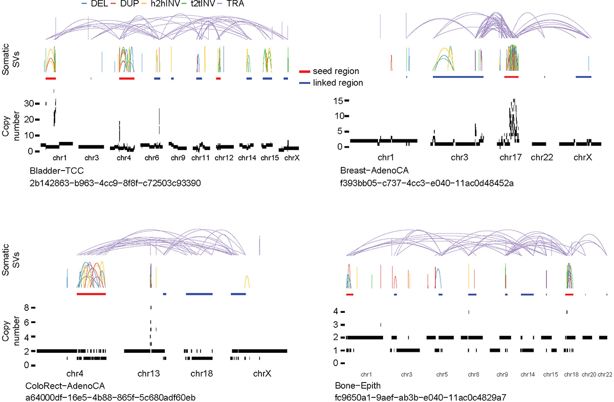
We hypothesize that the CGR copy-number pattern and distribution of breakpoints can be used to infer their mechanisms of formation. To this end, we developed a computational algorithm called “Starfish” to infer CGR signatures (see details in Methods). Briefly, we first selected 12 features to comprehensively depict the copy number and breakpoint patterns of each CGR (Fig. 1a). These features include breakpoint dispersion score, copy loss percentage, copy loss density, copy gain percentage, copy gain density, number of copy states, median copy number change, maximum copy number, highest telomere loss percentage, ratio of telomere loss and CGR loss, median breakpoint microhomology and median breakpoint insertion size. Features related to the magnitude of CGR events (i.e. number of chromosomes involved, number of rearrangements and size of CGR regions) were not used. After removing highly correlated features (Extended Data Fig. 2a) and features with small variances (Extended Data Fig. 2b), there were five features remaining: CGR breakpoint dispersion score (measuring the randomness of breakpoint distribution on chromosomes), copy loss percentage, copy gain percentage, telomere loss percentage and maximum copy number. We performed unsupervised consensus clustering for all 2,014 CGRs (Fig. 1a) using the five features and discovered six clusters (Fig. 1b and Extended Data Fig. 2c). Examples of CGRs are shown in Fig. 1c. Clusters constructed by different clustering approaches were very similar (Extended Data Fig. 2d). We use six clusters produced by the partition around medoids (PAM) algorithm for the remainder of this manuscript and refer to the clusters as CGR signatures (Supplementary Table 1). The CGR signatures jointly inferred based on their CNV and SV patterns are different from SNV or SV signatures deconvoluted using NMF. Our goal is to infer the molecular mechanisms of CGR formation, and therefore, we still use the term “signature” to reflect the similarity. We then trained a neural network classifier (Extended Data Fig. 3a), namely Starfish classifier, using the five features and CGR signature labels. For CGRs detected in additional samples, we can classify them into one of the CGR signatures derived from PCAWG samples.
Figure 1. Six CGR signatures detected in the PCAWG cohort.
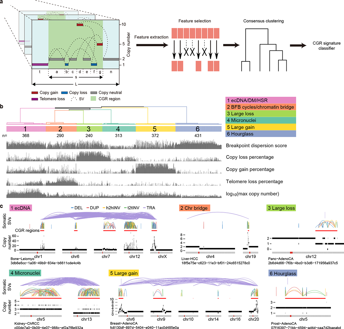
a, An overview of Starfish workflow. CGR regions are identified in PCAWG samples. Twelve features are selected to comprehensively describe the patterns of CGR events. Highly correlated features and features with low variability are removed. The remaining five features are used to perform unsupervised clustering. Once major clusters, referred to as CGR signatures, are detected from the PCAWG cohort, a CGR signature classifier is trained to assign additional CGRs to one of the six PCAWG signatures. The left most panel shows DNA copy number profiles (colored horizontal bars) and somatic SVs (dashed arcs) in CGR regions. Letters “a” to “g”, “n”, “t”, “s” and “L” in this panel denote the lengths of DNA segments. b, Six major clusters (CGR signatures) are detected from 2,014 CGRs in PCAWG cohort based on five features. The scores of five features are shown at the bottom. The numbers of CGRs in each signature are shown below the cluster IDs. c, Examples of CGRs from six signatures. In each example, chromosomes involved in CGRs are displayed side-by-side as grey bars at the bottom. The red dots in grey bars represent centromeres. The colored arcs on the top are five types of somatic SVs (deletions, duplications, head-to-head inversions, tail-to-tail inversions and translocations). CGR regions are marked by thick red lines below the SV arcs. Copy number profiles are shown below the CGR regions and above the chromosome bars. Tumor types and sample uuids are provided below the chromosome bars.
Benchmarking CGR Signatures
To link CGR signatures to known mechanisms, we took advantage of five studies that induced chromothripsis events through experimental approaches15–17,19,26. There were 186 whole-genome-sequenced single cells and cell clones in which micronuclei or chromatin bridges were observed in parental cells. We detected a total of 57 CGRs in these samples and predicted CGR signatures by Starfish classifier. In micronuclei samples, 63% of the CGRs (22 out of 35) were assigned to Signature 4, whereas in chromatin bridge samples, 64% of the CGRs (14 out of 22) were classified as Signature 2 (Fig. 2a and Supplementary Table 2). Signature 4 CGRs have the lowest breakpoint dispersion scores (i.e., breakpoints evenly distributed) with modest copy gains and losses (Fig. 1b), whereas Signature 2 CGRs highlight the largest amount of telomere loss (Fig. 1b). These properties are consistent with the molecular mechanisms of micronuclei- and chromatin-bridge-induced chromothripsis events. Some CGRs in Signature 2 display more than three copy states and may have undergone BFB cycles before dicentric chromosomes being resolved via chromatin bridge. Although micronuclei can result from chromatin bridge19, the mechanisms of DNA breakage in these aberrant structures are different. The chromosomes in micronuclei are shattered into many pieces due to nuclear envelope assembly defect27, whereas DNA breakage and local fragmentation of a chromatin bridge are caused by actomyosin-dependent mechanical force, and nuclear envelope rupture is not required19. The mechanistic difference leads to distinct patterns of chromothripsis. Micronuclei-induced chromothripsis events have even distribution of breakpoints, whereas bridge-induced events have localized breakpoints and are accompanied by loss of telomere. In the Umbreit et al. study, 13 CGRs formed via chromatin-bridge-induced micronuclei. Among these, 8 displayed patterns of Signature 4, similar to other micronuclei-induced chromothripsis (Fig. 2a). In summary, micronuclei- and chromatin-bridge-induced chromothripsis can be properly distinguished by Signatures 4 and 2.
Figure 2. Benchmarking CGR signatures.
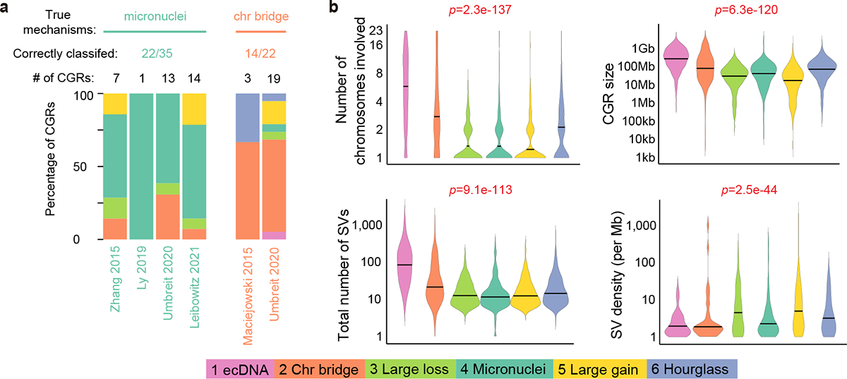
a, Benchmarking CGR signatures predicted by Starfish classifier using experimentally induced events. Each set of colored stacking bar represents CGRs detected from WGS data of one study. Different colors denote Starfish-predicted CGR signatures. b, Differences in magnitude of six CGR signatures. The colors of the violin plots denote CGR signatures. Horizontal lines in the violin plots are median values. P values are calculated by Kruskal-Wallis tests and shown with red texts if significant at the 0.05 level.
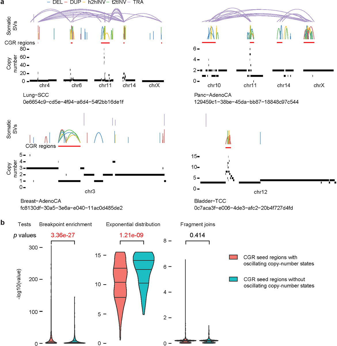
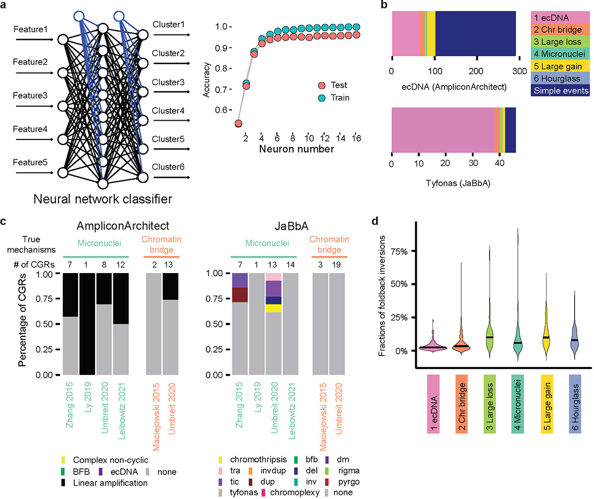
To associate CGR signatures with ecDNA, we utilized ecDNA predicted by AmpliconArchitect22 since 85% of the AmpliconArchitect-predicted ecDNA in cell lines were confirmed to be DMs by florescent in situ hybridization (FISH)22. In 289 AmpliconArchitect-predicted ecDNA from 849 tumors shared between this and the AmpliconArchitect studies, most were relatively simple (Extended Data Fig. 3b) as ecDNA/DM can form with only one DNA fragment ligated head-to-tail2,20. Out of the 100 complex circular events, 64 (64%) were classified as Signature 1 by Starfish. There were another 309 CGRs in Signature 1 not classified as ecDNA by AmpliconArchitect which could be the linear form of homogeneous staining regions (HSRs). To validate this, we compared them to tyfonas events predicted by JaBbA23 which were experimentally validated as HSRs. In 887 tumors shared by this and the JaBbA studies, 38 out of 46 (83%) JaBbA-predicted tyfonas events were classified as Signature 1 by Starfish (Extended Data Fig. 3b). These results combined suggest that the Signature 1 captures both ecDNA and HSRs. Signature 1 features highest maximum copy number with moderate percentages of copy gain (Fig. 1b) which is consistent with the properties of ecDNA and HSRs (small DNA fragments being highly amplified).
Since AmpliconArchitect and JaBbA can classify CGRs into different types, we applied both algorithms to the 57 experimentally induced CGRs from five studies15,17,19,26,28. Note that all three algorithms (Starfish, AmpliconArchitect and JaBbA) classify rearrangement types based on event patterns and not trained on experimental data. Starfish only used experimental data to name CGR signatures. AmpliconArchitect did not classify any of the micronuclei- or chromatin-bridge-induced chromothripsis as complex events or BFB (Extended Data Fig. 3c) as it was mainly designed to detect ecDNA. Most of the CGRs were unassigned by JaBbA with only one micronuclei-induced chromothripsis classified as chromothripsis (Extended Data Fig. 3c). Therefore, Starfish classifier performs better than existing algorithms when classifying micronuclei- and chromatin-bridge-induced chromothripsis. In summary, our CGR signature inference based on event patterns is highly accurate and biologically relevant.
We then investigated the differences in event magnitude among six CGR signatures. Signatures 1 and 2 have more chromosomes and SVs involved and affect larger genomic regions compared to the other signatures (Fig. 2b). The number of foldback inversions has been used to classify BFB-cycle events22,23. However, we found that the number of foldback inversions cannot effectively separate Signature 2 from others (Extended Data Fig. 3d).
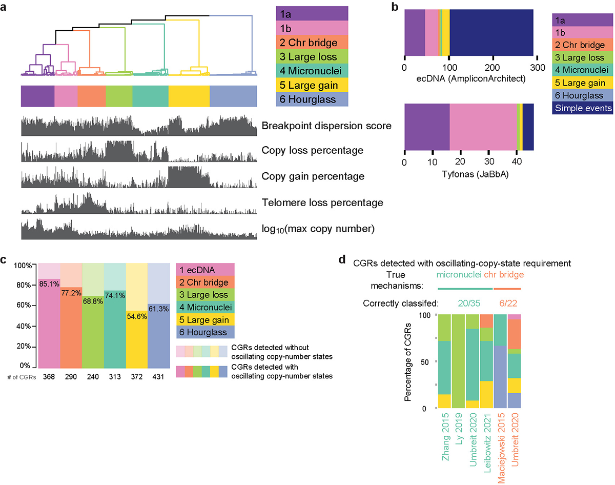
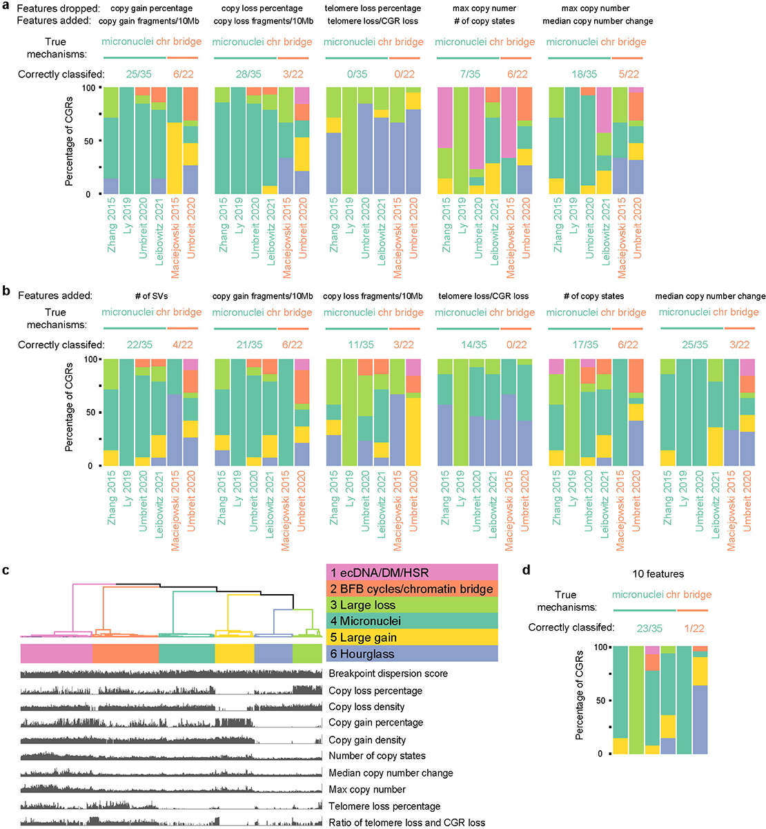
To further evaluate the performance of the six CGR signatures derived from the five features (Fig. 1b), we tested various alternatives. Firstly, if we clustered the CGRs into seven signatures, Signature 1 could be divided into two signatures 1a and 1b (Extended Data Fig. 4a), and both were mixtures of ecDNA and HSRs (Extended Data Fig. 4b). The main difference between ecDNA and HSRs are their topology (circular and linear), and therefore, graph-based approaches are better suited to distinguish them. Then, we evaluated the impact of our revision of CGR detection. Most CGRs of Signature 1 could be detected by the original version of ShatterSeek and discarding the oscillating-copy-number-state requirement (modified ShatterSeek) facilitated the detection of Signature 5 CGRs the most (Extended Data Fig. 4c). Our approach of CGR detection improved micronuclei- and chromatin-bridge-induced chromothripsis classification on experimentally induced cases (Extended Data Fig. 4d). To further test clustering using other features, we replaced one of the five features in Fig. 1b with another one or added an additional feature. The signatures identified are quite similar and the ones presented in Fig. 1b performs best when classifying ground-truth cases (Extended Data Fig. 5a,b). Using ten features to construct CGR signatures adds no benefit either (Extended Data Fig. 5c,d). Therefore, the six signatures constructed based on the five features we selected (Fig. 1b) are the optimal solution.
Figure 5. Biases of CGR breakpoints.
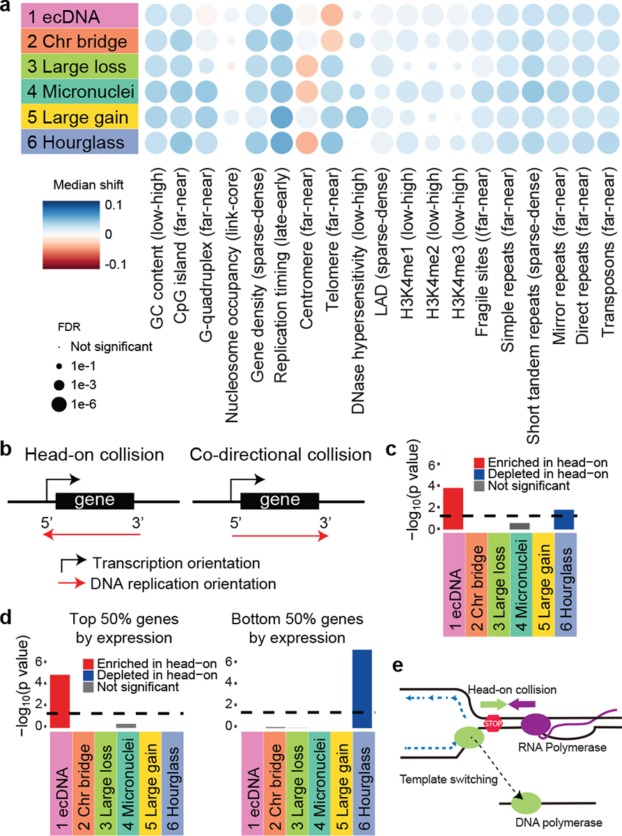
a, Associations of CGR breakpoints with various genomic properties. Median shift represents the difference between the observed and randomly shifted breakpoints in quantile distribution of the genomic property values. The direction of bias is noted in the parenthesis of each genomic property. For example, Signature 1 has negative median shift value for telomere which means Signature 1 breakpoints are far away from telomere. b, Scheme of transcription-replication collision. Head-on collision regions are defined as transcription and DNA replication orientations to be the opposite and co-directional collision regions are defined as transcription and DNA replication in the same orientation. c, Biases of CGR breakpoints in head-on collision regions. Bonferroni-corrected p values are calculated by comparing CGR breakpoints and randomly shuffled breakpoints in head-on/co-directional collision regions using two-sided Chi-square tests. d, Biases of CGR breakpoints in head-on collision regions controlled for gene expression level. P values are calculated by two-sided Chi-square test with Bonferroni correction. Dashed lines in c and d denote 0.05 corrected p value cutoff. e, Model of DNA polymerase switching template after transcription-replication collision. When DNA replication complex collides with transcription complex, replication fork collapses. DNA polymerase then switches template and continues replication. This process may be involved in ecDNA formation.
CGR signatures with unknown mechanisms and distribution of CGRs
There are three signatures that cannot be associated with any known biological processes. Signatures 3 and 5 present the largest amount of genomic copy losses and gains respectively (Fig. 1b,c). In sharp contrast, Signature 6 manifests the highest breakpoint dispersion scores (breakpoints unevenly distributed) with a very small amount of copy loss and no copy gain (Fig. 1b). We named this signature “hourglass chromothripsis” (Fig. 1c) due to the shape of its copy-number profile (small fractions of content leaking to the lower level). Note that Signatures 3, 5 and 6 are named based on their CNV and SV patterns but not their biological processes. Among the six signatures, Signature 6 is the most abundant one with 431 events in the PCAWG cohort while Signature 3 is the least common one with 240 events (Fig. 1b). More than half of the CGRs (1,043 out of 2,014, 52%) belong to the three signatures that cannot be attributed to any known mechanisms which highlights the advantage of our signature inference strategy.
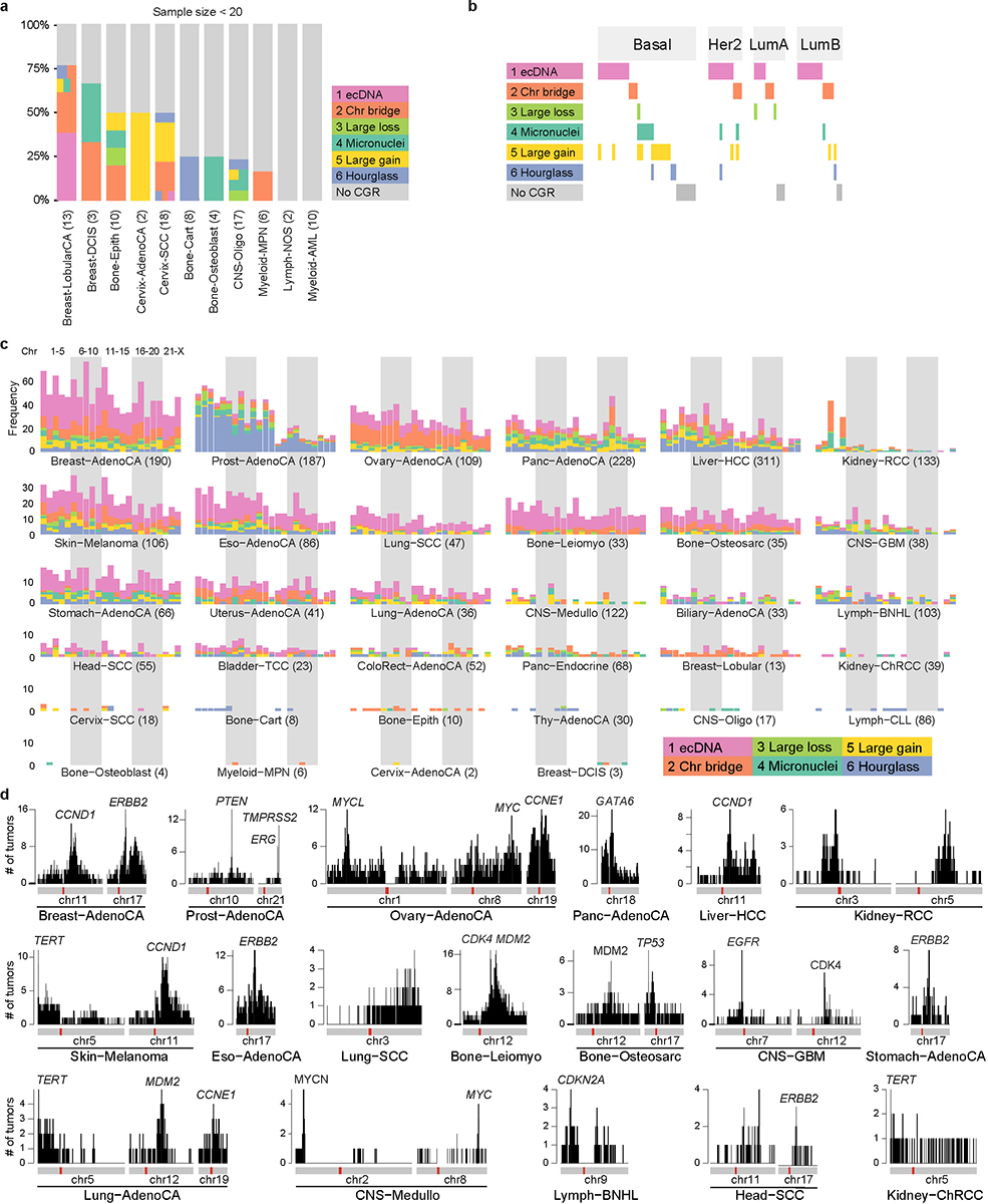
The frequencies of CGRs significantly vary across tumor types (Fig. 3a and Extended Data Fig. 6a). CGRs are most abundant in glioblastoma, osteosarcoma and esophageal cancer, while pilocytic astrocytoma and chronic lymphocytic leukemia barely have any. Signature 1 is frequently observed in many tumor types including various types of sarcoma, esophageal cancer and glioblastoma (Fig. 3a), which is consistent with previous studies21,22. In contrast, Signature 2 is most abundant in clear cell renal cell carcinoma (Fig. 3a) in which chromosomes 3 and 5 are known to be prone to chromothripsis29. This signature is also abundant in osteosarcoma and ovarian cancer (Fig. 3a). The enrichment of the Signatures 1 and 2 being consistent with previous studies again demonstrated the accuracy of our signature inference. Signature 6 is found in almost all tumor types (Fig. 3a) and is strikingly common in prostate cancer (107 out of 187, 57%). We also observed biases of CGR occurrences among tumor subtypes. For example, Signature 5 is enriched in basal breast cancers (Extended Data Fig. 6b). A total of 405 tumors have more than one CGR signatures (Fig. 3a).
Figure 3. Distribution of CGRs.
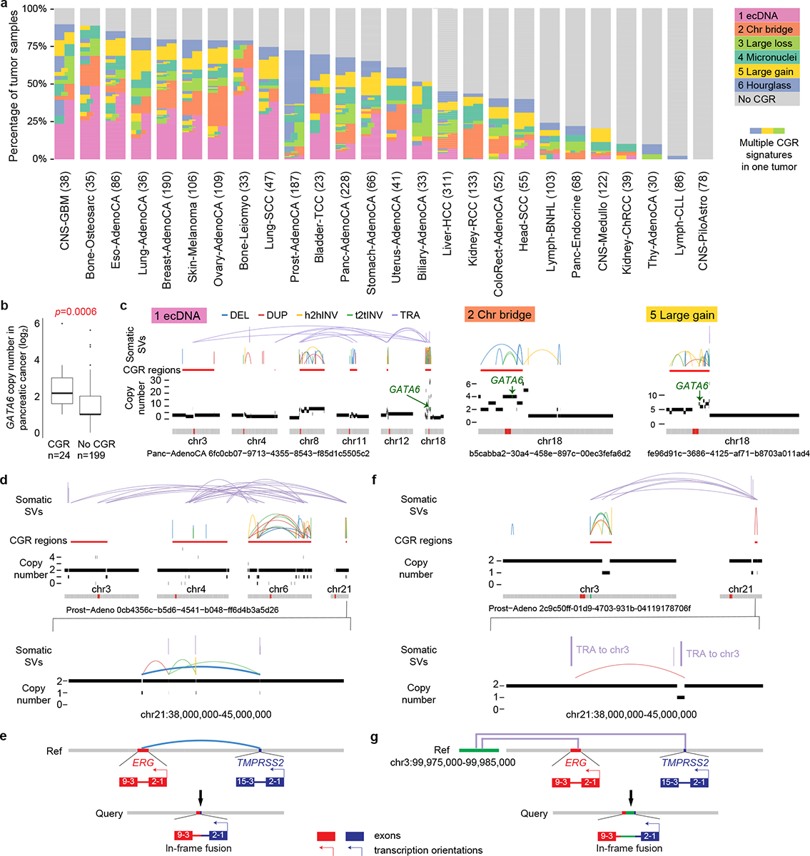
a, CGR occurrences in tumor types with at least 20 samples. Tumors are painted by CGR signatures. If one tumor carries more than one CGR signatures, it is painted by more than one colors horizontally. The height of each tumor may be different in different tumor types since all tumor types are scaled to the same height. Numbers in parenthesis denote sample sizes of the corresponding tumor types. b, GATA6 frequently amplified by CGRs in pancreatic cancers. Boxplot shows median value (thick black lines), upper and lower quartiles (boxes), 1.5x interquartile ranges (whiskers) and outliers (black dots) of log2(GATA6 copy numbers). P value is calculated by two-sided Wilcoxon rank sum test. c, Examples of GATA6 amplified by CGRs of different signatures in pancreatic cancers. Locations of GATA6 in three CGR regions are noted by green arrows. d-g, TMPRSS2-ERG fusions generated by CGRs in prostate cancer. d and f, SV and CNV profiles of two CGRs in prostate cancers. The lower panels show zoomed-in regions of TMPRSS2 and ERG on chromosome 21. Fusion-producing SVs are bolded. e and g, Reconstructions of fusions. Red and blue bars on the reference genome represent ERG and TMPRSS2 genes. Purple lines in g represent two translocations between chromosomes 3 and 21.
CGRs also have uneven distribution across the genome (Extended Data Fig. 6c). It was reported that regions with frequent CGRs often carry major cancer-driving genes, such as ERBB2 in breast cancer30 and EGFR in glioblastoma2. In fact, we were able to find cancer-driving genes in the majority of the CGR hotspots including CCND1, ERBB2, PTEN, TMPRSS2, MYCL, MYC, CCNE1, GATA6, TERT, CDK4, MDM2, TP53, EGFR, MYCN and CNKN2A (Extended Data Fig. 6d). GATA6 is known to be the most frequently amplified gene in pancreatic cancer31 and is an important subtype defining transcription factor32. The amplifications are often due to CGRs (Fig. 3b) of different signatures (Fig. 3c). Prostate cancers also have two CGR hotspots on chromosome 21 (Extended Data Fig. 6d) corresponding to fusions involving TMPRSS2 and ERG in seven tumors (Fig. 3d–g), even though most TMPRSS2-ERG fusions (84 out of 91) are caused by simple deletions. Therefore, a subset of CGRs are major drivers of tumorigenesis.
Genetic associations of CGRs
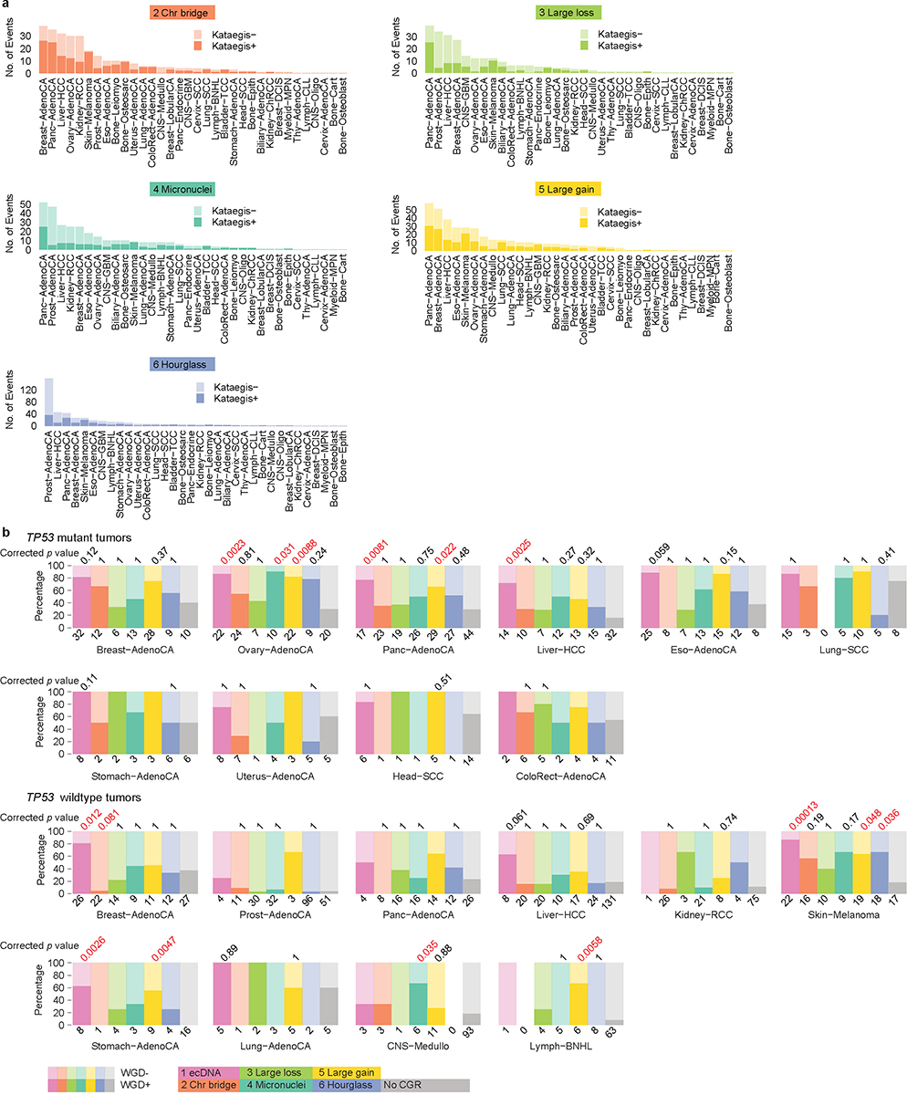
To better understand the mechanisms of CGR formation, we sought to identify genetic alterations associated with CGR signatures. It has been shown that TP53 mutations are associated with chromothripsis in tumors6,33. In cell line models, TP53 has to be inactivated so that the cells can tolerate chromothripsis without undergoing apoptosis15–17. We observed Signatures 1, 2, 4 and 5 are significantly associated with TP53 mutations (Fig. 4a) with FDRs of 3.5e-12, 2.2e-3, 4.5e-4 and 9.1e-12 respectively. When individual tumor types are tested, TP53 mutations remain to be associated with Signatures 1, 2, 4 and 5 in various tumor types (Supplementary Table 3). Interestingly, Signatures 3 and 6 (in an extended prostate cancer cohort) are significantly associated (FDRs 3.8e-2 and 5.9e-2 respectively) with mutations in Speckle Type BTB/POZ Protein (SPOP) (Fig. 4a), a subunit of an E3 ubiquitin ligase complex involved in protein ubiquitination and degradation. We will study Signature 6 in a greater detail in a later section.
Figure 4. Genetic associations of CGRs.
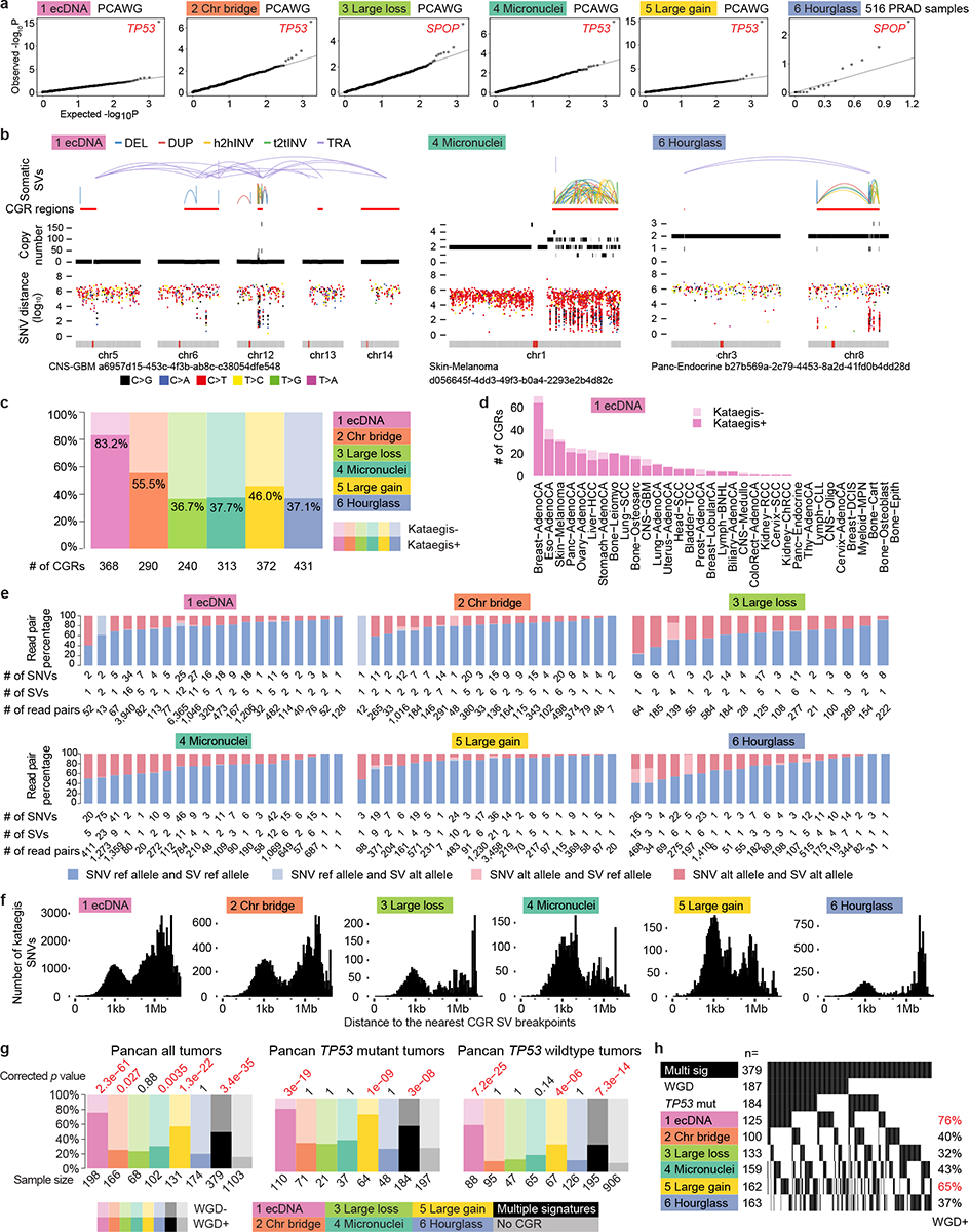
a, Q-Q plots of statistical associations between somatic mutations in protein-coding genes and CGR signatures. Each dot represents a gene. Observed and expected p values are calculated by two-sided Fisher’s exact tests and permutation tests. b, Examples of kataegis co-occurring with CGRs. Inter-mutational distances are shown below the SV and copy number profiles of CGRs. SNVs are colored by mutation types. Small distances indicate clustered SNVs. c, Percentages of CGRs with co-occurring kataegis. d, Frequencies of Signature 1 CGRs with and without co-occurring kataegis in different tumor types. e, Phasing kataegis SNVs and CGR SVs. Percentages of read pairs supporting reference alleles and alternative alleles for read pairs spanning closely located SNVs and SVs are shown in 20 randomly selected CGRs from each signature. There are only 15 phasable Signature 3 CGRs (at least one SNV/SV pair located within 1kb of each other) of which the raw sequencing data are available. f, Distributions of distances of kataegis SNVs to their nearest CGR SV breakpoints. g, Associations of CGR signatures with WGD. Each colored bar shows tumors carrying only one CGR signatures. Black and dark grey bars are tumors with multiple CGR signatures. The fractions of tumors with and without WGD are compared to samples without any CGRs (light grey bars on the right). P values are calculated by two-sided Fisher’s exact tests with Bonferroni correction and are shown on top of the bar plots. h, WGD frequencies in 379 tumors with multiple CGR signatures. The percentages on the right show the fractions of tumors to be WGD positive when carrying the corresponding CGRs. Tumors carrying either Signatures 1 or 5 are more likely to be WGD positive.
Kataegis, clustered somatic SNVs, occurs in 50% (1,004 out of 2,014) of the CGRs (Fig. 4b). Although kataegis is known to be associated with chromothripsis3,34 as a consequence of APOBEC3B activity18, we observed dramatic differences among six CGR signatures. The vast majority (83%) of Signature 1 CGRs are accompanied by kataegis in sharp contrast to about 40% in other signatures (Fig. 4c). Such enrichment is present in almost all tumor types (Fig. 4d). Interestingly, in melanoma, kataegis co-occurs with most of the CGRs regardless of their signatures (Fig. 4d and Extended Data Fig. 7a). We then randomly selected one chromosome from 20 CGRs of each signature in which we could phase the kataegis SNVs and CGR SVs using WGS data. In almost all cases, kataegis SNVs and CGR SVs are phased to the same DNA molecules (Fig. 4e). The distances between kataegis SNVs to the nearest CGR SVs display multi-modal distributions with three peaks at ~1kb, ~1Mb and ~10Mb (Fig. 4f). There are distinct differences across six signatures. Most CGR signatures have kataegis SNVs about 1kb and 1Mb away from SVs. However, there are hardly any kataegis SNVs at 1Mb distance from hourglass chromothripsis SVs, but many at about 10Mb distance. In addition, 24% and 32% of the kataegis SNVs are within 10kb of CGR SVs for Signatures 1 and 2, whereas a lot more (58% and 56%) kataegis SNVs are in that range for Signatures 4 and 5. A recent study18 reported that kataegis occurs on single-strand DNA resulting from the resolution of chromatin bridge and APOBEC3B may facilitate DNA fragmentation, whereas another study35 concluded that ecDNA-associated kataegis occurs after the amplification of ecDNA. If kataegis forms after the amplification of ecDNA, we would expect that a subset of reads/read pairs supporting CGR SVs do not carry kataegis SNVs. However, such reads/read pairs are very rare in the 20 Signature 1 CGRs we investigated (Fig. 4e). Similar trends are seen in all six signatures (Fig. 4e) which suggests that the majority of kataegis SNVs near CGR breakpoints are formed during CGR formation including ecDNA.
Aneuploidy can promote genome instability and chromothripsis36,37. When all tumors are considered, most CGR signatures are significantly associated with whole genome duplication (WGD) (Fig. 4g). However, when controlled for TP53 mutation status, only the tumors with Signatures 1 and 5 as well as the tumors with more than one CGR signature carry significantly more WGD (Fig. 4g). Among tumors with multiple CGR signatures, the ones harboring Signature 1 or 5 CGRs are more likely to carry WGD (Fig. 4h). We further investigated tumor-type-specific effects. Although sample sizes are limited, Signatures 1 and 5 remain significantly associated with WGD in several tumor types such as ovarian, pancreatic, stomach cancers and melanoma (Extended Data Fig. 7b). In summary, two CGR signatures, Signatures 1 and 5, are associated with WGD, while other signatures are not.
CGR breakpoint distribution biases
The uneven distribution of CGR breakpoints may provide clues for their formation. We observed that all CGRs are enriched in high GC content, high gene density and early-replicated regions (Fig. 5a) similar to most simple SVs38 suggesting that CGRs are more likely to form in open chromatin regions. The CGR breakpoints being closer to repetitive elements than expected (Fig. 5a) indicates that repetitive elements may play a role in DNA fragmentation and/or ligation during CGR formation. Interestingly, CGRs of Signatures 1 and 2 tend to occur far away from telomeres while CGRs of Signatures 3, 4, 5 and 6 preferentially occur near telomeres (Fig. 5a). It is possible that acentric DNA fragments resulted from breaks near the telomeres are more likely to produce micronuclei and chromothripsis.
Role of transcription-replication collision
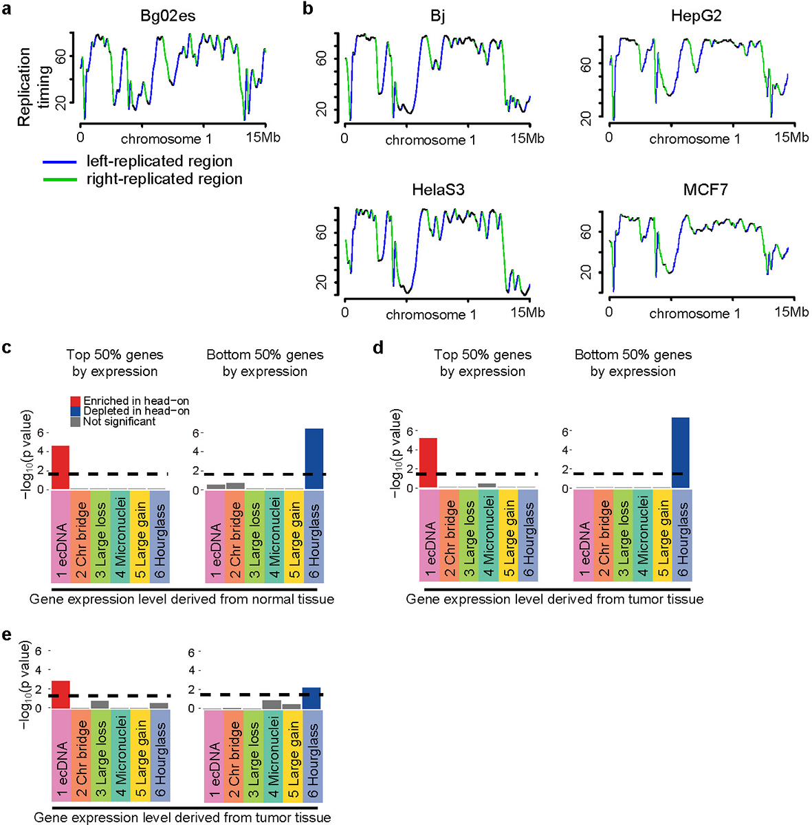
DNA replication stress is a major source of genome instability39. Collision between transcription and DNA replication machineries can result in replication fork collapse and genome instability40. Some very large genes, known as common fragile sites, are hotspots for deletions due to transcription-replication collision41. Recently, it was reported that deletions, insertions and point mutations can frequently form when such collisions are induced in bacteria42. Here, we sought to evaluate whether transcription-replication conflict contributes to CGRs in cancer. First, we defined left- and right-replicated regions based on RepliSeq data from cell line Bg02es (derived from human embryonic stem cells) as previously described43 (Extended Data Fig. 8a). These regions are largely conserved in different cell types (Extended Data Fig. 8b). Then, head-on and co-directional collision regions could be defined based on replication and transcription orientations (Fig. 5b). We found Signature 1 breakpoints are significantly enriched in head-on collision regions (Fig. 5c, Chi-square tests with Bonferroni correction) compared to randomly shuffled breakpoints. If the rearrangements are caused by transcription-replication conflict, we expect the enrichment depends on gene expression. When controlled for gene expression level, we indeed found the enrichment is only significant in top 50% of the genes (highly or moderately expressed) ranked by expression level in tumors, but not in the bottom 50% of the genes (lowly expressed or not expressed) (Fig. 5d). It is possible that the high gene expression is the consequence of CGRs. To rule out this possibility, we performed the same test using gene expression in normal tissues and observed a similar bias (Extended Data Fig. 8c). To further rule out the effect of selection, we removed breakpoints within 1 Mb of CGR hotspots (Extended Data Fig. 6d) and the bias could still be observed (Extended Data Fig. 8d). To control for tissue-specific differences in replication timing, we defined conserved left- and right-replicated regions using six solid-tissue-derived cell lines. Signature 1 breakpoints remain enriched in head-on collision regions depending on gene expression (Extended Data Fig. 8e). Previous studies based on in vitro experiments in cell lines reported that ecDNA can form via chromothripsis15,20. Our results indicated that the conflicts between DNA replication and transcription may contribute to ecDNA formation in tumor tissue. When a replication fork collapses, DNA polymerase can switch to a new template and different types of genomic rearrangements can form depending on the destination of the polymerase44. Template switching upon transcription-replication collision (Fig. 5e) can be a plausible alternative mechanism to produce circular DNA molecules. Further studies using experimental approaches are needed to elucidate the role of transcription-replication collision in ecDNA formation.
Hourglass chromothripsis in prostate cancer
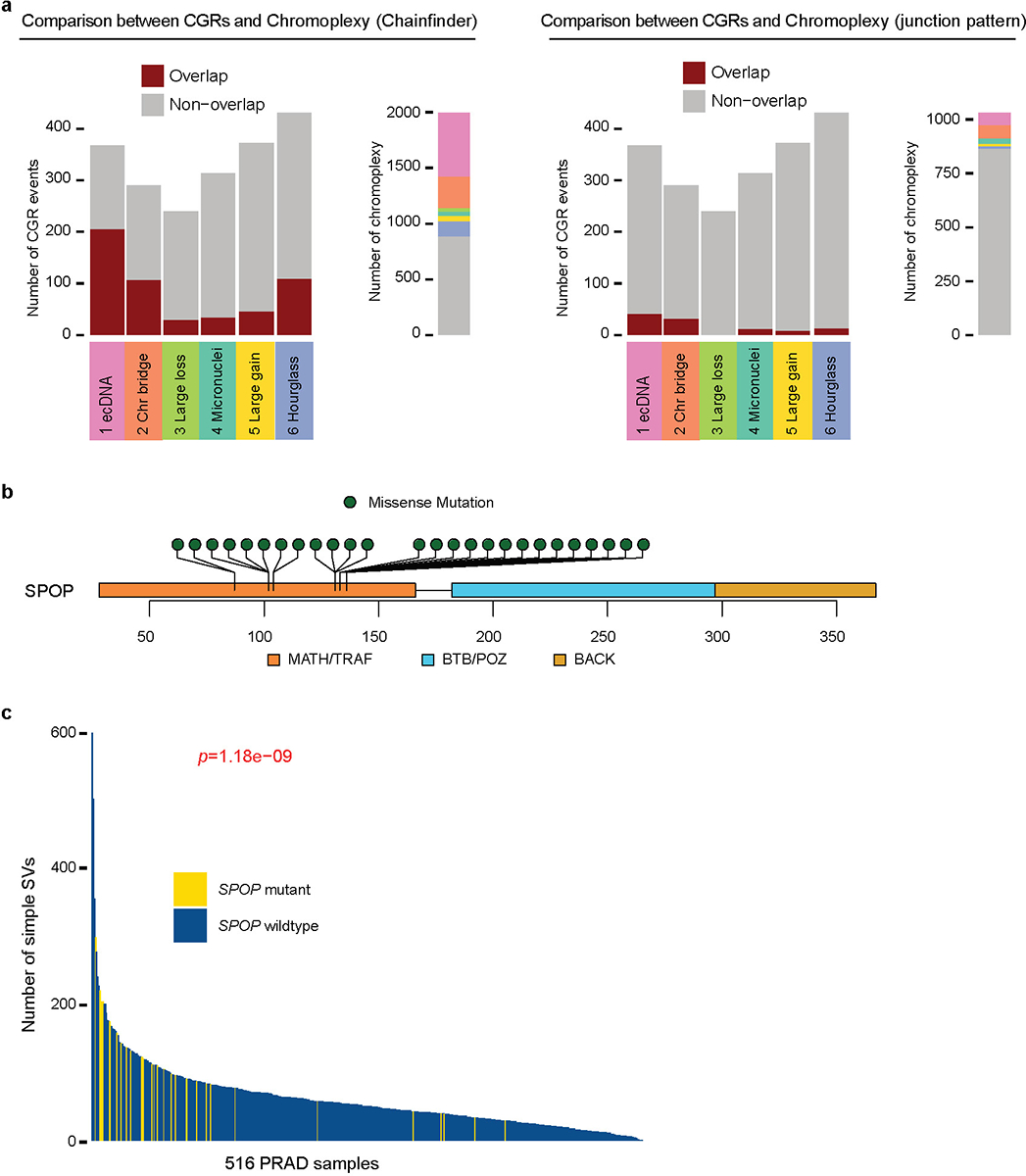
The Signature 6 hourglass chromothripsis is dominant in prostate cancer (Fig. 3a). Chromoplexy is another form of CGR enriched in prostate cancer3,9. It is considered to be the result of ligation of simultaneously broken DNA ends of several chromosomes9—a complex form of reciprocal translocations3. We sought to address whether hourglass chromothripsis is equivalent to chromoplexy. Using two strategies to detect chromoplexy: ChainFinder9 and junction patterns38, we found hourglass chromothripsis events have little overlap with chromoplexy (Extended Data Fig. 9a). In addition, most hourglass chromothripsis cases only involve one or two chromosomes (Fig. 2b) while chromoplexy usually involves multiple chromosomes9. Other than prostate cancer, hourglass chromothripsis is commonly seen in glioblastoma and bladder cancer (Fig. 3a), whereas chromoplexy is enriched in thyroid cancer and lymphoid malignancies3. Therefore, hourglass chromothripsis is a unique type of CGRs and distinct from chromoplexy.
To test whether hourglass chromothripsis is a one-time event, we utilized linked-read sequencing data of 23 prostate cancers45. We identified 10 hourglass chromothripsis events in 15 tumors including two in an SPOP mutant tumor 01115468-TA3. In this tumor, one hourglass chromothripsis occurred in chromosome 8 (Fig. 6a). Once the rearranged tumor chromosome was reconstructed based on somatic SVs (Fig. 6b), all rearranged DNA fragments could be phased into a single haplotype using linked-read barcodes. The same tumor harbored another more complex hourglass chromothripsis involving five chromosomes (Fig. 6c). We identified seven phased blocks with more than one somatic SVs. If hourglass chromothripsis results from simple SVs accumulated over time, we expect the somatic SVs to be evenly represented in different haplotypes. However, 144 out of the 155 somatic SVs in the seven phased blocks can be phased to one haplotype (Fig. 6d) which is extremely unlikely to occur by chance (p=1.3e-28, binomial tests, p values combined with Fisher’s method). These results suggest that hourglass chromothripsis events are indeed one-time catastrophic events.
Figure 6. Reconstruction of hourglass chromothripsis using linked-read sequencing data.
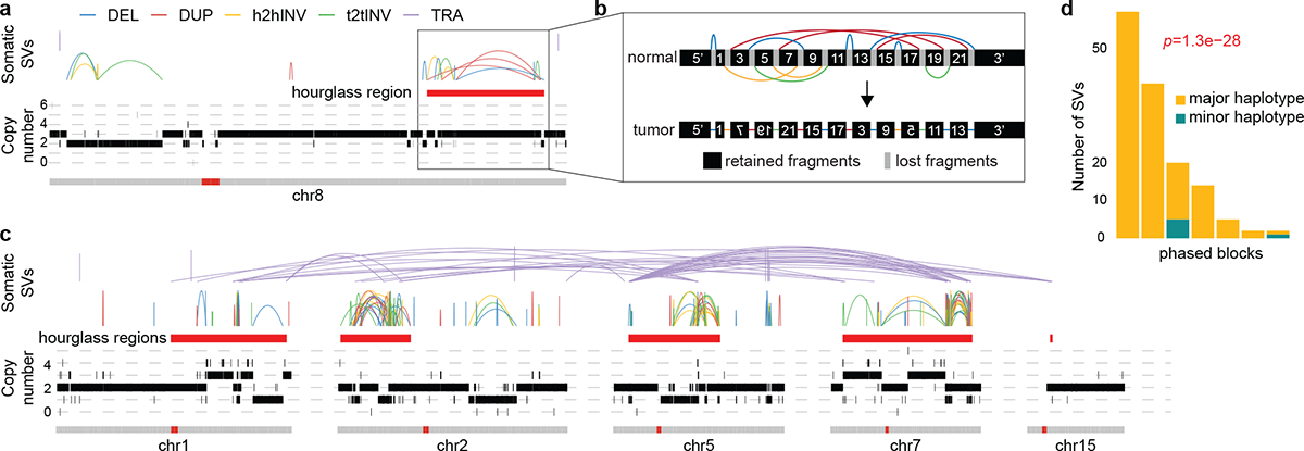
a, An hourglass chromothripsis on chromosome 8 in a prostate cancer with SPOP mutation. b, Reconstruction of hourglass chromothripsis in a in the tumor genome. Genomic segments are re-scaled for the chromothripsis region. The normal chromosome and SVs are shown on the top and the reconstructed tumor chromosome is shown at the bottom. Segments with flipped texts in tumor chromosome represent inverted DNA fragments. c, Another hourglass chromothripsis in the same tumor involving five chromosomes. d, Phasing somatic SVs in c using barcoded reads. Seven phased blocks with more than one somatic SVs are shown as vertical bars. Two-sided binomial test is performed in each of the seven phased blocks to test the enrichment of SVs in the major haplotype, and the p values are combined by Fisher’s method.
We then took advantage of additional 329 publicly available WGS prostate cancers from International Cancer Genome Consortium46,47 and identified another 359 CGRs (Supplementary Table 4). In the combined cohort of 516 prostate cancers, we found that somatic mutations in SPOP are significantly associated with hourglass chromothripsis (p=3.4e-3, Fisher’s exact test, Fig. 7a). SPOP is known to be recurrently mutated in prostate cancer and the mutations are mutually exclusive with ETS fusions (TMPRSS2-ERG, -ETV1, -ETV4 and -ETV5)48. All mutations are missense mutations in the meprin and TRAF homology (MATH) domain (Extended Data Fig. 9b) and potentially disrupt SPOP’s target binding. Signatures 3 and 4 are also associated with SPOP mutations (p=1.4e-10 and 1.5e-3, respectively, Fisher’s exact test; Fig. 7a). In addition, SPOP mutations are associated with elevated levels of simple genomic rearrangements (Extended Data Fig. 9c). Therefore, we conclude that SPOP may be a gatekeeper of genome stability. Mutant SPOP may allow the cells to tolerate various types of genomic rearrangements. Further experimental studies are needed to establish causal relationships of SPOP mutations and CGRs.
Figure 7. Hourglass chromothripsis in prostate cancer.
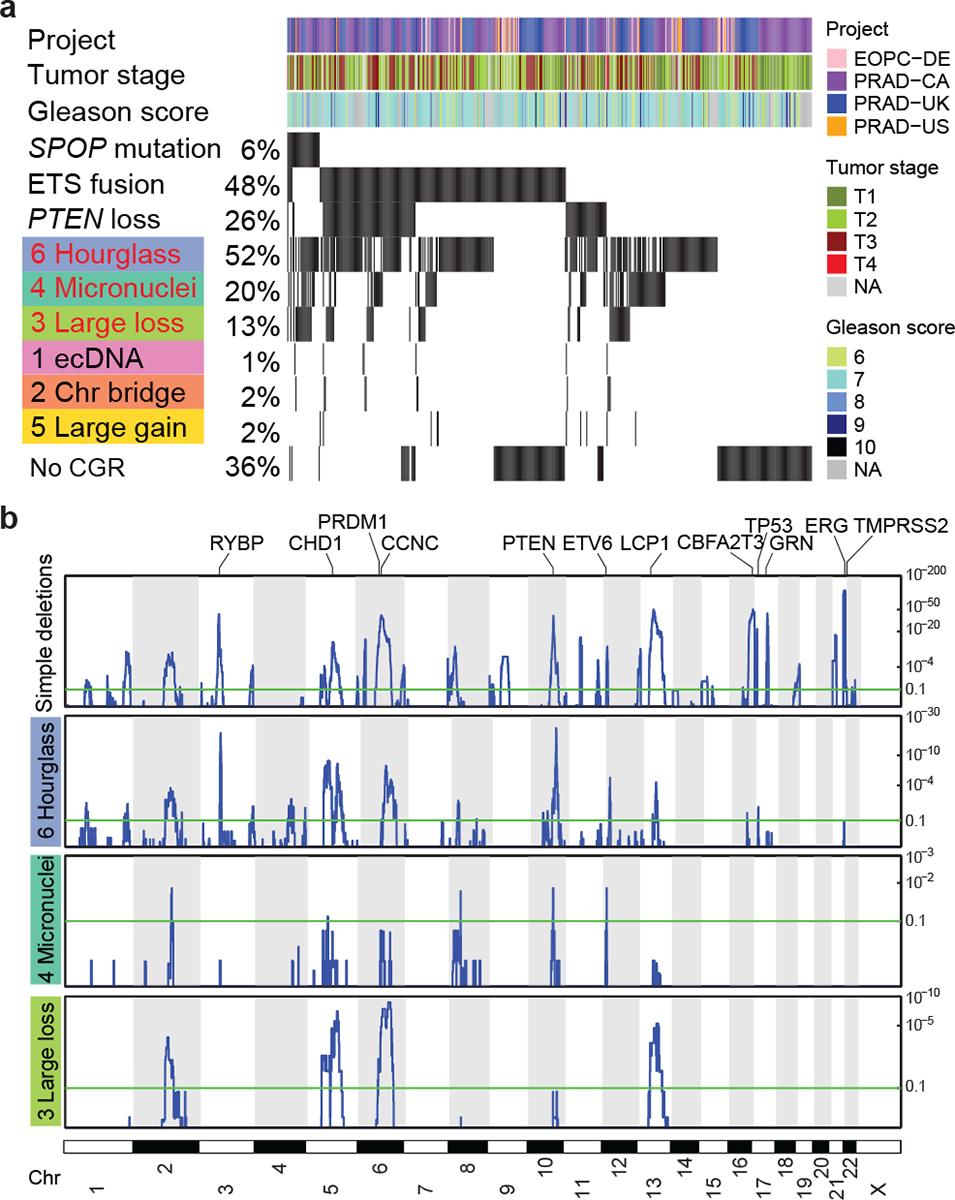
a, CGRs and genetic alterations in a combined cohort of 516 prostate cancers. Each track shows corresponding information for 516 tumors. Red texts depict CGR signatures significantly associated with SPOP somatic mutations. b, Recurrently deleted regions shown as blue peaks in four types of copy-loss-associated rearrangements in prostate cancer. Y axis shows q values.
Next, we sought to investigate the functional consequences of hourglass chromothripsis in prostate cancer. We identified recurrently deleted regions resulting from Signatures 3, 4 and 6 as well as simple deletions. We found that CGRs as well as simple deletions mostly delete the same regions leading to loss of tumor suppressors such as PTEN (Fig. 7b). This suggests that CGRs are under positive selection. A few peaks of simple deletions are not found in CGRs including the most frequent one in chromosome 21q22 (Fig. 7b) causing TMPRSS2-ERG fusions49. TMPRSS2-ERG fusions should be less likely to result from CGRs because both TMPRSS2 and ERG reside on chromosome 21 and are 3 Mb away from each other. The easiest way to form a fusion gene is through simple deletions. The chance of forming fusion gene via CGRs is expected to be much lower since DNA fragments in CGRs are randomly ligated. Nonetheless, we still observed four TMPRSS2-ERG fusions resulting from hourglass chromothripsis in 187 prostate cancers in the PCAWG cohort (Fig. 3d–g), which further suggested that hourglass chromothripsis promotes tumorigenesis in prostate cancer.
It is possible that hourglass chromothripsis is a special case of micronuclei-induced chromothripsis with less amount of DNA loss because both display oscillating copy number states. If both events are the results of random ligation of shattered DNA fragments, individual fragments being retained or lost should follow a Bernoulli distribution. In hourglass chromothripsis, larger fragments are always retained while smaller ones are always lost. If hourglass chromothripsis has the same forming mechanism as micronuclei-induced chromothripsis, hourglass chromothripsis should be rare. However, hourglass chromothripsis is more common than micronuclei-induced chromothripsis (Fig. 1b) which suggests that they are unlikely to form via random chromosomal shattering and ligation. In addition, the most dominant feature of hourglass chromothripsis is high breakpoint dispersion score while micronuclei-induced chromothripsis has the lowest score (Fig. 1b). Hourglass chromothripsis is abundant in prostate cancer while micronuclei-induced chromothripsis is not enriched in any tumor type (Fig. 3a). Intriguingly, the breakpoints of hourglass chromothripsis, but not micronuclei-induced chromothripsis, are depleted in the transcription-replication head-on collision regions only in the bottom 50% of the genes ranked by expression level but not in the top 50%, which is the opposite of ecDNA (Fig. 5d). These results indicate that the formation of hourglass chromothripsis might be associated with transcription-coupled repair. All of the above notable differences between hourglass and micronuclei-induced chromothripsis suggest that hourglass chromothripsis may have a distinct mechanism of formation.
Discussion
To study CGR forming mechanisms in human cancer using existing genomic sequencing data, there are two plausible approaches: train a computational model using ground-truth cases and classify CGRs detected from cancers; or classify CGRs detected from cancers and link them to known mechanisms. Here, we took the latter approach because the experimental studies on CGRs are still limited to only two mechanisms, and more importantly, the former approach would not allow us to detect types with unknown mechanisms. Our strategy does not rely on prior knowledge of CGR mechanisms, and the benchmarking results demonstrate high concordance with experimentally induced CGRs (Fig. 2a). Most CGR signatures have one dominant feature (Fig. 1b). So, some CGR events might be misclassified. For example, Signature 2 has the highest score in telomere loss (Fig. 1b) which is consistent with chromatin bridge mechanism17. If the breakpoint junction is too close to the telomere, the event would have low telomere-loss score and be misclassified as a different signature. Indeed, a fraction of CGRs are misclassified in benchmarking samples (Fig. 2a). Nevertheless, we were able to correctly classify most of the CGR events from five independent experimental studies (Fig. 2a) suggesting the good overall performance of Starfish classifier.
Several studies have shown that one mechanism can lead to many different types of rearrangements20,28,50 ranging from simple SVs, local jumps, BFB cycles to very complex rearrangements. Linking simple SVs to micronuclei or chromatin bridge would be extremely challenging. However, our study focuses on CGRs. The patterns of CGRs are distinct enough to be distinguished (Fig. 2a). Furthermore, when certain cell lines were exposed to drugs, various types of genomic alterations could be observed to confer resistance to drug such as arm-level copy gains, simple rearrangements, BFB cycles, chromothripsis and ecDNA with various configurations20. The experimental results demonstrated the exceeding complexity of genomic alterations. What we observe in human tumors is highly consistent with the experimental observation that one gene could be amplified through several distinct mechanisms (Fig. 3c). In our previous study, we have reported that EGFR in glioblastoma could be amplified as a single fragment in DM or co-amplified with many other fragments2. In many Signature 1 CGRs, some fragments in the CGR regions are amplified (e.g., chromosomes 1, 12 and X in Fig. 1c ecDNA of leiomyosarcoma) while others are not amplified or amplified at low levels (e.g., chromosomes 6 and 7 in Fig. 1c ecDNA of leiomyosarcoma). Our results also revealed unique features of ecDNA—their breakpoints are enriched in transcription and DNA replication head-on collision regions (Fig. 5c,d). This suggests that although ecDNA can form through micronuclei-induced and chromatin-bridge-induced chromothripsis events in vitro15,20, transcription activity and replication stress may play important roles in ecDNA formation during tumorigenesis.
Methods
Our research complies with all relevant ethical regulations.
Samples, variant calling and annotations
PCAWG WGS data for 2,428 tumor and matched-normal pairs across 37 cancer types (https://dcc.icgc.org/pcawg) from our previous study6 were used for the majority of this study unless otherwise noted. All variants (SNVs, CNVs, SVs, tumor purity, ploidy and WGD) for PCAWG samples were called by the PCAWG consortium using multiple algorithms3. Kataegis was detected by SeqKat (https://cran.r-project.org/web/packages/SeqKat/index.html). Additional 329 WGS prostate cancers from ICGC were used to study CGRs in prostate cancer. Somatic variants in these samples were downloaded from ICGC data portal (https://dcc.icgc.org/). For linked-read sequencing data of 23 prostate cancers45, somatic SNVs and SVs were obtained from the previous study45, copy number segments were identified by BIC-Seq54, and integer copy number was calculated by Sequenza55. CpG island annotation was downloaded from UCSC Genome Table Browser (genome.ucsc.edu/cgi-bin/hgTables). G-quadruplex (G4) clusters and fragile site positions were obtained from previous studies51,52. Nucleosome occupancy (mean values at 5 base-pair resolution) of K562 cell line, replication timing of NHEK (derived from normal skin) cell line, DNase hypersensitivity (average imputed negative log p-value in 1 kb window) of GM12878 cell line, histone modifications (average signal values in 1 kb window) of Gm12878 cell line, and repeat sequence annotations were downloaded from UCSC Genome Table Browser (genome.ucsc.edu/cgi-bin/hgTables). Lamina associated domain (LAD) (proportion of bases in 1 Mb window) in the Tig3 cell line of normal human embryonic lung fibroblasts were obtained from a previous study53. Replication timing profiles for Bg02es, Bj, HelaS3, HepG2, IMR90 and MCF7 cell lines were obtained from ENCODE (https://www.encodeproject.org/). Gene expression levels (upper-quartile-normalized fragments per kb per million mapped reads [FPKM-UQ]) of tumor tissues were available from PCAWG and gene expression levels of normal tissues (only a subset of tumor types have matched-normal tissues) from the Cancer Genome Atlas (TCGA) samples were downloaded from Genomic Data Commons (https://portal.gdc.cancer.gov/). All coordinates were based on hg19 reference genome. GENCODE v19 was used for gene annotation.
Identification of CGRs
Modified ShatterSeek6 was used to identify CGR “seed” regions based on interleaved SVs, chromosomal enrichment test, exponential distribution of breakpoints test and fragment joins test. Oscillating-copy-state criteria was removed from the original ShatterSeek package. In each sample, linked regions were identified if they were connected by at least two translocations within 10 kb of any seed regions. The search was performed iteratively until no new linked regions could be found. Finally, a CGR event was defined as all connected seed and linked regions combined (Extended Data Fig. 10). The somatic SVs of CGR were defined as all inter-chromosomal translocations and interleaved intra-chromosomal SVs in the CGR regions. The remaining SVs were defined as simple SVs.
CGR signature inference
Twelve features were initially selected to comprehensively describe the patterns of 2,014 CGR events including breakpoint dispersion score, copy loss percentage, copy loss density (number of copy loss fragments per 10Mb, log scale), copy gain percentage, copy gain density (number of copy gain fragments per 10Mb, log scale), number of copy states (log scale), median copy number change (log scale), maximum copy number (log scale), highest telomere loss percentage, ratio of telomere loss and CGR loss (log scale), median breakpoint microhomology (log scale), and median breakpoint insertion size (log scale). In Fig. 1a, the size of CGR region [s] equals to . Breakpoint dispersion score was defined as mean absolute deviation of [a:g] which measured the randomness of breakpoint distribution of a CGR. Copy loss and copy gain percentages were calculated by /[s] and (/[s]. Copy loss and copy gain densities were length[b,f]/([s]/10Mb) and length[d,g]/([s]/10Mb). Telomere loss percentage was t/L. All values were converted to z scores. To reduce collinearity among these features, the features with high correlation (abs(correlation coefficient)>0.5) were removed, including copy loss density, copy gain density, number of copy states, median copy number change, and ratio of telomere loss and CGR loss. Features with small variance were further removed including median breakpoint microhomology and median breakpoint insertion size. After feature selection process, five features were kept for downstream analysis: breakpoint dispersion score, copy loss percentage, copy gain percentage, maximum copy number and highest telomere loss percentage. Then, a 2,014 × 5 matrix was constructed for all CGRs. Four clustering methods (k-means based on Euclidean distance, partitioning around medoids [PAM] based on Euclidean distance, hierarchical clustering based on Pearson distance, and hierarchical clustering based on Euclidean distance) were used to perform unsupervised clustering. Optimal cluster number K and the best clustering method were determined based on four scores: Silhouette score, C-index, Calinski-Harabasz score, and Dunn-index. The K maximizing the ratio of intra-cluster similarity/inter-cluster similarity was selected. The final clustering was performed by R package “Consensuscluster Plus” using PAM with 0.9 item and 5000 iterations.
Neural network classifier (Starfish classifier)
The feature matrix and CGR signature labels from Fig. 1b were used to construct a signature classifier. The R package “neuralnet” was used to train a one layer neural-network classifier with 5-fold cross validation using 70% of CGR events as the training data and 30% of them as the validation data for each iteration. One to sixteen neurons were used in each iteration with 10e6 steps to converge at the error of 0.01. The model with 8 neurons was selected.
Benchmarking using experimentally induced chromothripsis
A total of 186 WGS samples from five published studies15–17,19,26 were used to benchmark our CGR signatures. Somatic SVs and CNVs were obtained from the corresponding publications. The CGRs were detected as described above. The feature matrices from individual studies were combined with PCAWG feature matrix and normalized. The CGR signatures were predicted using the Starfish classifier. AmpliconArchitect and JaBbA were used to analyze these samples with default parameters. All three tools were compared on the same CGRs detected by the modified ShatterSeek. Clustering, classification and benchmarking using CGRs detected by the original version of Shatterseek or using different features were conducted the same way as using five features.
Associations of CGR signatures
Co-occurrence and mutual exclusivity of CGR signatures were tested using DISCOVER package56. Oncogenes and tumor suppressors were collected from Cancer Gene Census57.
Protein-coding gene mutation status and the presence/absence of CGR signatures were used to construct two by two contingency tables across all PCAWG samples. Only genes mutated in more than 10 tumors were considered. Fisher’s exact test was used to compute p values and false discovery rate was computed by Benjamini- Hochberg procedure for each CGR signature. Significant genes were selected by FDR<0.1. Mutation status was permuted using R package “QQperm” with 1000 iterations to calculate expected p values and generate Q-Q plots.
CGR signatures in prostate cancers
The CGR signatures were predicted in 329 ICGC prostate cancers46,47 and 23 prostate cancers sequenced by linked reads45 as described in the benchmarking section using the Starfish classifier. Recurrently deleted regions were identified by GISTIC58.
CGR breakpoint enrichment analysis
Two random SVs were generated for each CGR SV by fixing the SV size and orientation and then placing them randomly to uniquely mappable regions of the same chromosome. Distances to CpG islands and G4 structures were log10 transformed. Gene density was calculated as the proportion of bases in protein-coding genes in 1 Mb window based on GENCODE v19. The density of short tandem repeats was calculated as the proportion of bases belonging to short tandem repeats in a 3 kb window. For each genomic property, a quantile distribution for the genomic property values at the observed breakpoints and randomly shuffled breakpoints were generated and the median shift was calculated as “the median quantile of observed breakpoints” minus “the median quantile of shuffled breakpoints”. A Kolmogorov-Smirnov test was conducted to compare normalized genomic property values from observed and random breakpoints, and a Benjamini-Yekutieli correction for false discovery rate was performed.
Transcription-replication collision
Left- and right-replicated regions were defined as regions where the changes of replication timing were more than 0.02 per kb (Extended Data Fig. 8a). In Bg02es, a total of 10,421 genes were in left- or right-replicated regions. Conserved regions were defined as those consistently annotated as left- or right-replicated in at least three out of the six cell lines. A total of 9,422 genes were in conserved regions. Transcription orientations were derived using gene annotation of GENCODE v19. Only breakpoints in protein-coding genes were considered. Breakpoints in overlapping genes of different orientations were discarded. Median expression levels of protein-coding genes within each tumor type were used. The numbers of SV breakpoints observed in tumors and the numbers of randomly generated SV breakpoints were used to test breakpoint enrichment in head-on collision regions using Chi-square test with Bonferroni correction.
Reconstruction of hourglass chromothripsis using linked reads
Phased blocks were inferred in the tumor samples by Long Ranger based on heterozygous SNVs (both germline and somatic) and barcoded reads. The barcoded reads with at least three heterozygous SNVs were retrieved to assign unique haplotypes by gemtools59. Somatic SVs in the tumor samples were phased using barcodes and shared SNVs. Phased blocks were further merged if they shared at least ten barcoded read pairs or were connected by at least two somatic SVs. The haplotype contained more SVs was assigned as the major haplotype and the other one was assigned as the minor haplotype. Binomial test was performed in each of the seven phased blocks with more than one somatic SVs to test the enrichment of SVs in the major haplotype, and the p values were combined by Fisher’s method.
Statistics & Reproducibility
No statistical method was used to predetermine sample size, but our sample sizes are similar to those reported in previous publications6,45–47. No data were excluded from the analyses. The experiments were not randomized. The Investigators were not blinded to allocation during experiments and outcome assessment. Data distribution was assumed to be normal but this was not formally tested. Further information on research design is available in the Nature Research Reporting Summary linked to this article.
Extended Data
Extended Data Fig. 1. Modification of Shatterseek by removing oscillating-copy-number-state requirement.
a, Examples of CGRs not detected by the original version of ShatterSeek. The SV and copy number profiles are shown for four CGRs. CGR regions are marked by red bars below SVs. b, Comparisons between CGR seed regions detected with and without oscillating-copy-state requirement. Breakpoint enrichment test is a binomial test corrected for mappability to evaluate the enrichment of SVs in each chromosome. Exponential distribution test evaluates whether the distribution of SV breakpoints differ from an exponential distribution. The smaller p values for breakpoint enrichment test and exponential test the better. Fragment joins test evaluates whether the distribution of DNA fragment joins diverges from a multinomial distribution with equal probabilities for each category using the goodness-of-fit test for the multinomial distribution. The larger p values for fragment joins test the better. FDR correction was performed on all p values. The newly detected CGRs without oscillating-copy-state have better p values for exponential distribution test and comparable p values for fragment joins test compared to CGRs detected by the original Shatterseek. CGRs detected with oscillating-copy-state have better p values in breakpoint enrichment test because more CGRs of Signatures 1 and 2 are detected with oscillating-copy-state (Figure S4c) and these CGRs have more SVs (Figure 2b). Although the newly detected CGRs are less enriched in each chromosome, they all pass the Shatterseek p value cutoff. N = 3,996 CGR seed regions.
Extended Data Fig. 2. Clustering of CGRs.
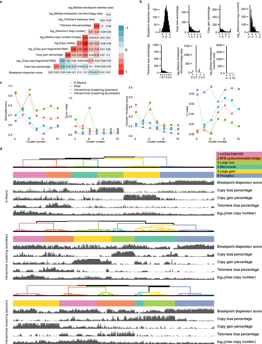
a, Correlation heatmap of twelve genomic features. The colors and numbers represent the correlation coefficients. b, Distributions of seven genomic features with low correlations. The x axes are normalized Z scores. Two features (median breakpoint microhomology size and median breakpoint insertion size) have low variations and are not used in the clustering step. c, Four indexes to evaluate number of clusters. d, Unsupervised clusters produced by three clustering methods (K-means, Hierarchical clustering with Euclidean distance and Hierarchical clustering with Pearson distance). N = 2014 CGRs.
Extended Data Fig. 3. Starfish classifier and benchmarking CGR signatures.
a, A neural network classifier (Starfish classifier) to classify any given CGRs into one of the six signatures derived from the PCAWG cohort. The left panel shows the scheme of neural network classifier, and the right panel shows performance of the neural network classifier. b, Comparison between ecDNA predicted by AmpliconArchitect, tyfonas events predicted by JaBbA, and CGR Signature 1. N = 289 Circular events, 46 tyfonas events and 368 ecDNA CGRs. c, CGRs classified by AmpliconArchitect and JaBbA in five experimental studies. The raw sequencing data, which is required by AmpliconArchitect, are not available for several samples. Therefore, the number of CGRs classified by AmpliconArchitect is less than that of Starfish and JaBbA. d, Fractions of foldback inversions in six CGR signatures. N = 791 CGRs.
Extended Data Fig. 4. Performances of other clustering approaches.
a, Seven clusters formed using five features. Signature 1 splits into two clusters (1a and 1b). b, Comparisons of Signatures 1a and 1b to ecDNA detected by AmpliconArchitect and HSRs detected by JaBbA. c, Proportions CGRs detected with and without oscillating-copy-state requirement. d, Benchmarking CGR classification if unmodified Shatterseek is used to detect CGRs.
Extended Data Fig. 5. Performances of clustering using different features.
a, Benchmarking CGR classification by replacing one feature from the five used in Figure 1b. b, Benchmarking CGR classification by adding one feature. N = 57 CGRs. c, Six clusters formed using ten features. All features related to CGR CNV and SV properties are used. The SV breakpoint microhomology and insertion size are not used because these measures are not available in the experimentally induced CGRs. d, Benchmarking CGR classification by using ten features. In each benchmarking test in a, b and d, CGRs from five experimental studies are used. Each colored bar shows CGRs classified with the corresponding features in each study. The numbers of corrected classified CGRs and total CGRs are displayed above the bars.
Extended Data Fig. 6. Distribution of CGRs.
a, CGR frequencies in tumor types with less than 20 samples. Tumors are painted by CGR signatures. If one tumor carries more than one CGR signatures, it is painted by more than one colors horizontally. The height of each tumor may be different in different tumor types since all tumor types are scaled to the same height. b, Occurrences of CGRs in four breast cancer subtypes. N = 74 tumors. c, Frequencies of CGRs per chromosome in different tumor types. CGRs from chromosomes 1 to X are shown with 23 bars and painted by their signatures. The numbers after tumor types denote sample sizes. d, CGR breakpoint hotspots and cancer-driving genes. CGR breakpoint frequencies on most frequent chromosomes for 18 tumor types. Each vertical line represents the number of tumors having CGR breakpoints in a 100 kb window.
Extended Data Fig. 7. Kataegis and WGD co-occuring with CGRs.
a, Numbers of CGRs with and without co-occurring kataegis in each tumor type stratified by five CGR signatures. Signature 1 is shown in Figure 3d. b, Percentages of tumors with and without WGD stratified by TP53 mutation status, tumor type and CGR signature. Only tumor types with at least five samples in no CGR group and at least five samples in any one of the CGR signature group are displayed. P values calculated by two-sided Fisher’s exact test with Bonferroni correction are shown above the CGR signatures with at least five samples. The ones significant at 0.05 level are labelled in red. The numbers at the bottom of each graph represent the number of samples.
Extended Data Fig. 8. Transcription-replication collision and CGR breakpoints.
a, Defining DNA replication orientations based on replication-timing profile of Bg02es cell line. b, Replication timing profiles and replication orientations in four other cell lines (Bj, HepG2, HelaS3 and MCF7). c, Breakpoint biases in six CGR signatures stratified by gene expression level from normal tissues. d, CGR breakpoint biases after excluding breakpoints within 1 Mb of CGR hotspots. e, CGR breakpoint biases computed using conserved left- and right-replicated regions identified from six cell lines. In c, d and e, p values are calculated by comparing observed breakpoints and randomly shuffled breakpoints in head-on and co-directional collision regions using two-sided Chi-square tests. Bonferroni corrections are performed. Dashed lines represent the 0.05 p value cutoff.
Extended Data Fig. 9. Hourglass chromothripsis in prostate cancer.
a, Six CGR signatures compared to ChainFinder-predicted and junction-pattern-predicted chromoplexy events. N = 1991 ChainFinder-predicted events, 1031 junction-pattern-predicted chromoplexy events and 2014 CGRs. b, Somatic mutation distribution in SPOP gene in prostate cancer. All mutations are missense mutations in the MATH/TRAF domain which is the target binding domain. c, Number of simple SVs in prostate cancers with and without SPOP mutations. P value is calculated by two-sided Wilcoxon rank sum test. N = 516 PRAD samples.
Extended Data Fig. 10. Identification of CGR seed and linked regions.
Genomic regions satisfying interleaved SVs, goodness-of-fit, fragment joins test, chromosomal enrichment test, and exponential distribution of breakpoints test using the ShatterSeek package are defined as CGR seed regions. Linked regions are defined as regions connected to seed regions by at least two translocations. All seed and linked regions combined are defined as one CGR event.
Supplementary Material
Acknowledgement
We thank the Center for Research Informatics at the University of Chicago for providing the computing infrastructure and Matthew Stephens, Xin He and Michelle Le Beau for helpful suggestions. The work was supported by the National Institutes of Health grant K22CA193848 (LY) and University of Chicago and UChicago Comprehensive Cancer Center (LY).
Footnotes
Code availability
The Starfish package is available at https://github.com/yanglab-computationalgenomics/Starfish.
Competing interests
The authors have no competing interests to declare.
Data availability
Raw sequencing data for 329 ICGC prostate cancers are available at European Genome-phenome Archive with the accession code EGAS00001000900 and EGAS00001000262. Linked-read WGS on 23 prostate cancer were obtained from dbGAP with the identifier phs001577.v1.p1. Source data have been provided as Source Data files. All other data supporting the findings of this study are available from the corresponding author on reasonable request.
References
- 1.Negrini S, Gorgoulis VG & Halazonetis TD Genomic instability — an evolving hallmark of cancer. Nat. Rev. Mol. Cell Biol 11, 220–228 (2010). [DOI] [PubMed] [Google Scholar]
- 2.Yang L et al. Diverse mechanisms of somatic structural variations in human cancer genomes. Cell 153, 919–929 (2013). [DOI] [PMC free article] [PubMed] [Google Scholar]
- 3.Campbell PJ et al. Pan-cancer analysis of whole genomes. Nature 578, 82–93 (2020). [DOI] [PMC free article] [PubMed] [Google Scholar]
- 4.Conrad DF et al. Origins and functional impact of copy number variation in the human genome. Nature 464, 704–712 (2009). [DOI] [PMC free article] [PubMed] [Google Scholar]
- 5.Stephens PJ et al. Massive genomic rearrangement acquired in a single catastrophic event during cancer development. Cell 144, 27–40 (2011). [DOI] [PMC free article] [PubMed] [Google Scholar]
- 6.Cortés-Ciriano I et al. Comprehensive analysis of chromothripsis in 2,658 human cancers using whole-genome sequencing. Nat. Genet 52, 331–341 (2020). [DOI] [PMC free article] [PubMed] [Google Scholar]
- 7.Liu P et al. Chromosome catastrophes involve replication mechanisms generating complex genomic rearrangements. Cell 146, 889–903 (2011). [DOI] [PMC free article] [PubMed] [Google Scholar]
- 8.Holland AJ & Cleveland DW Chromoanagenesis and cancer: mechanisms and consequences of localized, complex chromosomal rearrangements. Nat. Med 18, 1630–1638 (2012). [DOI] [PMC free article] [PubMed] [Google Scholar]
- 9.Baca SC et al. Punctuated evolution of prostate cancer genomes. Cell 153, 666–677 (2013). [DOI] [PMC free article] [PubMed] [Google Scholar]
- 10.Giardiello FM et al. Guidelines on genetic evaluation and management of lynch syndrome: A consensus statement by the us multi-society task force on colorectal cancer. Gastroenterology 147, 502–526 (2014). [DOI] [PubMed] [Google Scholar]
- 11.Fong PC et al. Inhibition of Poly(ADP-Ribose) Polymerase in Tumors from BRCA Mutation Carriers. N. Engl. J. Med 361, 123–134 (2009). [DOI] [PubMed] [Google Scholar]
- 12.Alexandrov LB et al. Deciphering Signatures of Mutational Processes Operative in Human Cancer. Cell Rep 3, 246–259 (2013). [DOI] [PMC free article] [PubMed] [Google Scholar]
- 13.Macintyre G et al. Copy number signatures and mutational processes in ovarian carcinoma. Nat. Genet 50, 1262–1270 (2018). [DOI] [PMC free article] [PubMed] [Google Scholar]
- 14.Chiang C et al. The impact of structural variation on human gene expression. Nat. Genet 49, 692–699 (2017). [DOI] [PMC free article] [PubMed] [Google Scholar]
- 15.Zhang C-Z et al. Chromothripsis from DNA damage in micronuclei. Nature 522, 179–184 (2015). [DOI] [PMC free article] [PubMed] [Google Scholar]
- 16.Ly P et al. Selective Y centromere inactivation triggers chromosome shattering in micronuclei and repair by non-homologous end joining. Nat. Cell Biol 19, 68–75 (2017). [DOI] [PMC free article] [PubMed] [Google Scholar]
- 17.Maciejowski J, Li Y, Bosco N, Campbell PJ & de Lange T Chromothripsis and Kataegis Induced by Telomere Crisis. Cell 163, 1641–1654 (2015). [DOI] [PMC free article] [PubMed] [Google Scholar]
- 18.Maciejowski J et al. APOBEC3-dependent kataegis and TREX1-driven chromothripsis during telomere crisis. Nat. Genet 52, 884–890 (2020). [DOI] [PMC free article] [PubMed] [Google Scholar]
- 19.Umbreit NT et al. Mechanisms generating cancer genome complexity from a single cell division error. Science 368, eaba0712 (2020). [DOI] [PMC free article] [PubMed] [Google Scholar]
- 20.Shoshani O et al. Chromothripsis drives the evolution of gene amplification in cancer. Nature 591, 137–141 (2020). [DOI] [PMC free article] [PubMed] [Google Scholar]
- 21.Turner KM et al. Extrachromosomal oncogene amplification drives tumour evolution and genetic heterogeneity. Nature 543, 122–125 (2017). [DOI] [PMC free article] [PubMed] [Google Scholar]
- 22.Kim H et al. Extrachromosomal DNA is associated with oncogene amplification and poor outcome across multiple cancers. Nat. Genet 52, 891–897 (2020). [DOI] [PMC free article] [PubMed] [Google Scholar]
- 23.Hadi K et al. Distinct Classes of Complex Structural Variation Uncovered across Thousands of Cancer Genome Graphs. Cell 183, 197–210.e32 (2020). [DOI] [PMC free article] [PubMed] [Google Scholar]
- 24.Korbel JO & Campbell PJ Criteria for inference of chromothripsis in cancer genomes. Cell 152, 1226–1236 (2013). [DOI] [PubMed] [Google Scholar]
- 25.Li Y et al. Constitutional and somatic rearrangement of chromosome 21 in acute lymphoblastic leukaemia. Nature 508, 98–102 (2014). [DOI] [PMC free article] [PubMed] [Google Scholar]
- 26.Leibowitz ML et al. Chromothripsis as an on-target consequence of CRISPR–Cas9 genome editing. Nat. Genet 53, 895–905 (2021). [DOI] [PMC free article] [PubMed] [Google Scholar]
- 27.S L et al. Nuclear envelope assembly defects link mitotic errors to chromothripsis. Nature 561, 551–555 (2018). [DOI] [PMC free article] [PubMed] [Google Scholar]
- 28.P L et al. Chromosome segregation errors generate a diverse spectrum of simple and complex genomic rearrangements. Nat. Genet 51, 705–715 (2019). [DOI] [PMC free article] [PubMed] [Google Scholar]
- 29.Mitchell TJ et al. Timing the Landmark Events in the Evolution of Clear Cell Renal Cell Cancer: TRACERx Renal. Cell 173, 611–623 (2018). [DOI] [PMC free article] [PubMed] [Google Scholar]
- 30.Yang L et al. Analyzing Somatic Genome Rearrangements in Human Cancers by Using Whole-Exome Sequencing. Am. J. Hum. Genet 98, 843–856 (2016). [DOI] [PMC free article] [PubMed] [Google Scholar]
- 31.Raphael BJ et al. Integrated Genomic Characterization of Pancreatic Ductal Adenocarcinoma. Cancer Cell 32, 185–203 (2017). [DOI] [PMC free article] [PubMed] [Google Scholar]
- 32.Chan-Seng-Yue M et al. Transcription phenotypes of pancreatic cancer are driven by genomic events during tumor evolution. Nat. Genet 52, 231–240 (2020). [DOI] [PubMed] [Google Scholar]
- 33.Rausch T et al. Genome sequencing of pediatric medulloblastoma links catastrophic DNA rearrangements with TP53 mutations. Cell 148, 59–71 (2012). [DOI] [PMC free article] [PubMed] [Google Scholar]
- 34.Yang L et al. An enhanced genetic model of colorectal cancer progression history. Genome Biol 20, 168 (2019). [DOI] [PMC free article] [PubMed] [Google Scholar]
- 35.Bergstrom EN et al. Mapping clustered mutations in cancer reveals APOBEC3 mutagenesis of ecDNA. Nature 602, 510–517 (2022). [DOI] [PMC free article] [PubMed] [Google Scholar]
- 36.Ganem NJ, Godinho SA & Pellman D A mechanism linking extra centrosomes to chromosomal instability. Nature 460, 278–282 (2009). [DOI] [PMC free article] [PubMed] [Google Scholar]
- 37.Dewhurst SM et al. Tolerance of whole- genome doubling propagates chromosomal instability and accelerates cancer genome evolution. Cancer Discov 4, 175–185 (2014). [DOI] [PMC free article] [PubMed] [Google Scholar]
- 38.Li Y et al. Patterns of somatic structural variation in human cancer genomes. Nature 578, 112–121 (2020). [DOI] [PMC free article] [PubMed] [Google Scholar]
- 39.Macheret M & Halazonetis TD DNA replication stress as a hallmark of cancer. Annu. Rev. Pathol. Mech. Dis 10, 425–448 (2015). [DOI] [PubMed] [Google Scholar]
- 40.García-Muse T & Aguilera A Transcription-replication conflicts: How they occur and how they are resolved. Nat. Rev. Mol. Cell Biol 17, 553–563 (2016). [DOI] [PubMed] [Google Scholar]
- 41.Helmrich A, Ballarino M & Tora L Collisions between Replication and Transcription Complexes Cause Common Fragile Site Instability at the Longest Human Genes. Mol. Cell 44, 966–977 (2011). [DOI] [PubMed] [Google Scholar]
- 42.Sankar TS, Wastuwidyaningtyas BD, Dong Y, Lewis SA & Wang JD The nature of mutations induced by replication-transcription collisions. Nature 535, 178–181 (2016). [DOI] [PMC free article] [PubMed] [Google Scholar]
- 43.Haradhvala NJ et al. Mutational Strand Asymmetries in Cancer Genomes Reveal Mechanisms of DNA Damage and Repair. Cell 164, 538–549 (2016). [DOI] [PMC free article] [PubMed] [Google Scholar]
- 44.Carvalho CMB et al. Replicative mechanisms for CNV formation are error prone. Nat. Genet 45, 1319–1327 (2013). [DOI] [PMC free article] [PubMed] [Google Scholar]
- 45.Viswanathan SR et al. Structural Alterations Driving Castration-Resistant Prostate Cancer Revealed by Linked-Read Genome Sequencing. Cell 174, 433–447 (2018). [DOI] [PMC free article] [PubMed] [Google Scholar]
- 46.Fraser M et al. Genomic hallmarks of localized, non-indolent prostate cancer. Nature 541, 359–364 (2017). [DOI] [PubMed] [Google Scholar]
- 47.Wedge DC et al. Sequencing of prostate cancers identifies new cancer genes, routes of progression and drug targets. Nat. Genet 50, 682–692 (2018). [DOI] [PMC free article] [PubMed] [Google Scholar]
- 48.Abeshouse A et al. The Molecular Taxonomy of Primary Prostate Cancer. Cell 163, 1011–1025 (2015). [DOI] [PMC free article] [PubMed] [Google Scholar]
- 49.Tomlins SA et al. Recurrent fusion of TMPRSS2 and ETS transcription factor genes in prostate cancer. Science 310, 644–648 (2005). [DOI] [PubMed] [Google Scholar]
- 50.SM D et al. Structural variant evolution after telomere crisis. Nat. Commun 12, 2093 (2021). [DOI] [PMC free article] [PubMed] [Google Scholar]
- 51.Yoshida W et al. Identification of G-quadruplex clusters by high-throughput sequencing of whole-genome amplified products with a G-quadruplex ligand. Sci. Rep 8, 3116 (2018). [DOI] [PMC free article] [PubMed] [Google Scholar]
- 52.Kumar R et al. HumCFS: A database of fragile sites in human chromosomes. BMC Genomics 19, 985 (2019). [DOI] [PMC free article] [PubMed] [Google Scholar]
- 53.Guelen L et al. Domain organization of human chromosomes revealed by mapping of nuclear lamina interactions. Nature 453, 948–951 (2008). [DOI] [PubMed] [Google Scholar]
- 54.Xi R et al. Copy number variation detection in whole-genome sequencing data using the Bayesian information criterion. Proc. Natl. Acad. Sci. U. S. A 108, E1128–E1136 (2011). [DOI] [PMC free article] [PubMed] [Google Scholar]
- 55.Favero F et al. Sequenza: allele-specific copy number and mutation profiles from tumor sequencing data. Ann. Oncol 26, 64–70 (2015). [DOI] [PMC free article] [PubMed] [Google Scholar]
- 56.Canisius S, Martens JWM & Wessels LFA A novel independence test for somatic alterations in cancer shows that biology drives mutual exclusivity but chance explains most co-occurrence. Genome Biol 17, 1–17 (2016). [DOI] [PMC free article] [PubMed] [Google Scholar]
- 57.Sondka Z et al. The COSMIC Cancer Gene Census: describing genetic dysfunction across all human cancers. Nat. Rev. Cancer 18, 696–705 (2018). [DOI] [PMC free article] [PubMed] [Google Scholar]
- 58.Mermel CH et al. GISTIC2.0 facilitates sensitive and confident localization of the targets of focal somatic copy-number alteration in human cancers. Genome Biol 12, R41 (2011). [DOI] [PMC free article] [PubMed] [Google Scholar]
- 59.Greer SU & Ji HP Structural variant analysis for linked-read sequencing data with gemtools. Bioinformatics 35, 4397–4399 (2019). [DOI] [PMC free article] [PubMed] [Google Scholar]
Associated Data
This section collects any data citations, data availability statements, or supplementary materials included in this article.
Supplementary Materials
Data Availability Statement
Raw sequencing data for 329 ICGC prostate cancers are available at European Genome-phenome Archive with the accession code EGAS00001000900 and EGAS00001000262. Linked-read WGS on 23 prostate cancer were obtained from dbGAP with the identifier phs001577.v1.p1. Source data have been provided as Source Data files. All other data supporting the findings of this study are available from the corresponding author on reasonable request.