

Abstract
Objective
Foodborne diseases pose a significant public health concern globally. This study aims to analyze the correlation between disease prevalence and climatic conditions, forecast the pattern of foodborne disease outbreaks, and offer insights for effective prevention and control strategies and optimizing health resource allocation policies in Guizhou Province.
Methods
This study utilized the χ2 test and four comprehensive prediction models to analyze foodborne disease outbreaks recorded in the Guizhou Foodborne Disease Outbreak system between 2012 and 2022. The best-performing model was chosen to forecast the trend of foodborne disease outbreaks in Guizhou Province, 2023–2025.
Results
Significant variations were observed in the incidence of foodborne disease outbreaks in Guizhou Province concerning various meteorological factors (all P≤0.05). Among all models, the SARIMA-ARIMAX combined model demonstrated the most accurate predictive performance (RMSE: Prophet model=67.645, SARIMA model=3.953, ARIMAX model=26.544, SARIMA-ARIMAX model=26.196; MAPE: Prophet model=42.357%, SARIMA model=37.740%, ARIMAX model=15.289%, SARIMA-ARIMAX model=13.961%).
Conclusion
The analysis indicates that foodborne disease outbreaks in Guizhou Province demonstrate distinct seasonal patterns. It is recommended to concentrate prevention efforts during peak periods. The SARIMA-ARIMAX hybrid model enhances the precision of monthly forecasts for foodborne disease outbreaks, offering valuable insights for future prevention and control strategies.
Keywords: Foodborne disease outbreaks, Climatic influence, ARIMAX model, Combination forecasting model.
A foodborne disease outbreak occurs when two or more cases of a similar clinical illness arise from a common food source, as determined by epidemiological investigations, or when such exposure results in one or more fatalities (1). Outbreaks of foodborne illnesses exert a more profound impact on individuals, families, and public health systems compared to isolated incidents of foodborne illnesses (2). Forecasting future patterns of foodborne disease outbreaks can facilitate the provision of healthcare resources, inform targeted interventions, and help prioritize preventative measures (3-4). The incidence of foodborne diseases is influenced by multiple factors, including the immune competence of individuals, improper food handling practices, and characteristics of the pathogens involved (5). Additionally, with the ongoing trend of global warming, the interplay between foodborne diseases and climate change is becoming more pronounced. Nevertheless, domestic research exploring the link between weather patterns and foodborne disease outbreaks is sparse. Moreover, some predictive studies of foodborne disease outbreaks have overlooked meteorological variables (6).
This study aims to develop a prediction model utilizing data from the “Guizhou Foodborne Disease Outbreak Surveillance System” between 2012 and 2022. The objective is to forecast future trends, identify crucial prevention and control measures for foodborne disease outbreaks in Guizhou Province, and lay the foundation for crafting prevention and control strategies, early warning systems, and health resource distribution policies. The ultimate goal is to decrease the frequency of foodborne disease outbreaks and mitigate associated risks.
METHODS
This study utilized data from the “Guizhou Foodborne Disease Outbreak Surveillance System” at the Guizhou Center for Disease Control and Prevention. Meteorological data from the World Weather Information Service (http://worldweather.wmo.int/zh/home.html) and China Weather Network (http://www.weather.com.cn) were collected for each city and state in Guizhou Province from 2012 to 2022. Five monthly average weather indicators were analyzed: average monthly rainfall, average monthly rainfall days, average monthly relative humidity, monthly relative humidity, and average hours of sunshine.
The data was organized using Excel 2019 (Microsoft, Redmond, WA, US), and SPSS 24.0 (IBM, Armonk, NY, US) was utilized to perform the χ2 test for the reported prevalence of foodborne disease outbreaks. The statistical analysis considered differences to be significant at P<0.05. The rate of foodborne disease outbreaks was the dependent variable, while climate factors were the independent variables. Each climate factor was categorized into five groups based on its magnitude. The χ2 test was employed to assess the statistical significance of differences in disease rates among the various factor groups.
Due to the seasonal patterns of foodborne disease outbreaks and their correlation with climatic conditions, this research utilized the seasonal autoregressive integrated moving average (SARIMA) model. The study also applied the autoregressive integrated moving average with exogenous regressors (ARIMAX) model and a combination of SARIMA-ARIMAX models (7). The Prophet model served as a reference for comparison. Given the complexity of the analysis process with fewer random variables (8), a substantial sample size spanning from 2012 to 2022 was necessary for reliable results. The time series prediction model was developed using R 4.2.2 (R Core Team, Vienna, Austria), with parameters selected for model fitting assessment (9).
RESULTS
Prevalence of Foodborne Disease Outbreaks in Guizhou Province in Climatic Conditions
For the investigation into foodborne disease outbreaks under varied climatic conditions, the study classified average monthly rainfall into five categories: from 5 to 65.2 mm, 65.2 to 125.4 mm, 125.4 to 185.6 mm, 185.6 to 245.8 mm, and 245.8 to 306 mm. The number of rainy days per month was similarly grouped: 4 to 7.2 days, 7.2 to 10.4 days, 10.4 to 13.8 days, 13.8 to 16.8 days, and 16.8 to 20 days. Average monthly temperature was divided into the ranges of 2.7 to 8.6 °C, 8.6 to 14.5 °C, 14.5 to 20.4 °C, 20.4 to 26.3 °C, and 26.3 to 32.2 °C. For monthly relative humidity, the categories were set from 62.0% to 66.8%, 66.8% to 71.6%, 71.6% to 76.4%, 76.4% to 81.2%, and 81.2% to 86.0%. Lastly, average sunshine hours per month were categorized into ranges of 1.8 to 3.06 hours, 3.06 to 4.32 hours, 4.32 to 5.58 hours, 5.58 to 6.84 hours, and 6.84 to 8.1 hours. The χ2 test results revealed statistically significant differences in the incidence rates of foodborne disease outbreaks across the various climatic categories in Guizhou Province from 2012 to 2022. The χ2 values are respectively: 2,122.142, 1,066.166, 2,753.543, 1,656.289, and 1,739.290, all P≤0.001 (Supplementary Table S1, available at https://weekly.chinacdc.cn/).
Results of Predictive Model
Based on the Prophet model: According to Supplementary Figure S1 (available at https://weekly.chinacdc.cn/), the prediction plot generated by the Prophet model (Supplementary Figure S1A) displayed that all predicted values fell within the 95% confidence interval (CI). The assessment metrics indicated a good fit of the Prophet model with RMSE=67.645 and MAPE=42.357%. This demonstrates the model's capability in capturing the general incidence trend and seasonal patterns of foodborne disease outbreaks. The upper segment of Supplementary Figure S1B suggests a potential increasing trend in foodborne illnesses in Guizhou Province in the future. The lower segment of Figure S1B illustrates the seasonal pattern of foodborne disease outbreaks, highlighting a peak season from June to September.
Based on the SARIMA model: In this study, 16 SARIMA models were finally listed, and three better models were selected for the series based on the AIC and BIC criteria. Each of the three models is expressed as SARIMA (1,1,1) (0,1,1)12, SARIMA (0,1,2) (1,1,1)12, SARIMA (0,1,2) (1,1,1)12. The BIC values for the three models were 1,317.555, 1,322.103, and 1,321.861; the AIC values were 1,306.864, 1,308.739, and 1,308.497, respectively. For the three alternative models initially selected, RMSE and MAPE were used as the main prediction accuracy evaluation indexes, and the RMSE values of the three models were 53.953, 60.489, and 62.301, respectively; and the MAPE values were 37.740%, 36.021%, and 37.209%, respectively. A comprehensive comparison of the AIC and BIC values of the alternative models revealed that the SARIMA (1,1,1) (0,1,1)12 model is the best, as can be seen in its prediction graph, fits well with the actual reported values (Supplementary Figure S2, available at https://weekly.chinacdc.cn/).
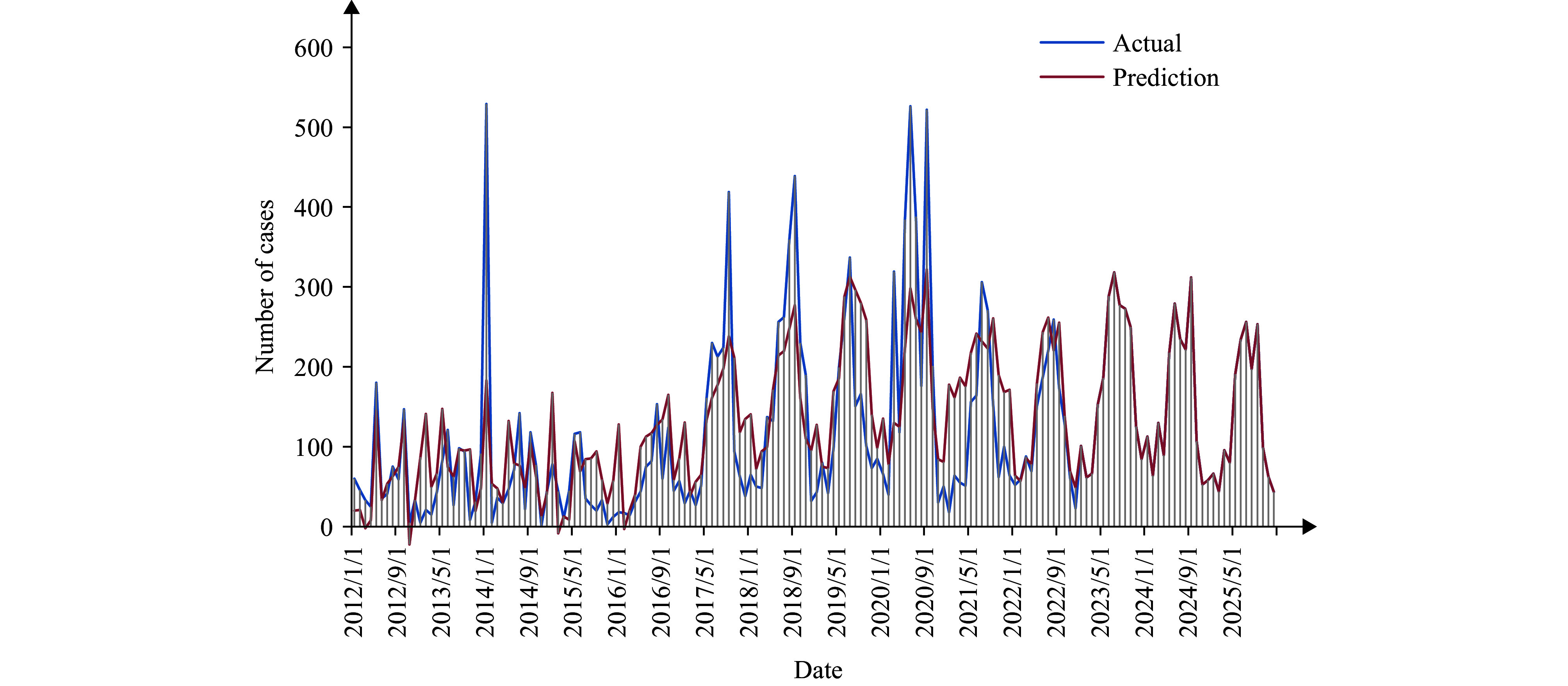
Based on the ARIMAX model: In this study, 16 ARIMAX models were evaluated, and three models were chosen based on AIC and BIC criteria. The selected models are ARIMAX (1,1,1) (0,1,1), ARIMAX (0,1,1) (0,1,1), and ARIMAX (1,1,1) (1,1,1). The BIC values for these models were 1,321.170, 1,325.520, and 1,324.470, while the AIC values were 1,308.400, 1,310.320, and 1,309.270, respectively. RMSE and MAPE were used to assess prediction accuracy, with the RMSE values being 26.544, 28.614, and 67.999, and the MAPE values being 15.289%, 20.441%, and 44.102%, respectively. Comparing the AIC and BIC values, the model ARIMAX (1,1,1) (0,1,1) was found to be the best, showing good agreement with actual data (Supplementary Figure S3, available at https://weekly.chinacdc.cn/).
Based on the SARIMA-ARIMAX combination model: The RMSE and MAPE values were used to compare the predictive performance of two models simultaneously. The optimal sub-models selected were SARIMA (1,1,1) (0,1,1)12 with a MAPE value of 37.740% and ARIMAX (1,1,1) (0,1,1) with a MAPE value of 15.289%. Weight coefficients of 0.246 and 0.654 were assigned to the SARIMA and ARIMAX models, respectively, based on calculations. The expression for the combined SARIMA-ARIMAX model is:
 |
The respective predictive outputs of two submodels are weighted according to their associated coefficients and then aggregated to determine the forecast of the combined SARIMA-ARIMAX model. This integrated approach was employed to model the occurrence of foodborne disease outbreaks in Guizhou Province from 2012 to 2022. The resulting fitted data aligned well with the original trend (Supplementary Figure S4, available at https://weekly.chinacdc.cn/). Data from foodborne disease outbreaks between January and December 2022 constituted the test set. Evaluation of this test set indicated that the combined SARIMA-ARIMAX model achieved RMSE of 26.196 and MAPE
Comparison of Forecasting Models
Upon a thorough examination of the prediction curves of various models forecasting the occurrence of foodborne disease outbreaks in Guizhou Province from January to December 2022, it is evident that all models' projected values align closely with the actual data. Analyzing the RMSE and MAPE metrics, the SARIMA, ARIMAX, and SARIMA-ARIMAX models developed in this study outperform the benchmark Prophet model. Additionally, the ARIMAX model surpasses the SARIMA model individually, while the combined SARIMA-ARIMAX model excels over the three standalone models. Forecasts using the optimal SARIMA-ARIMAX model for 2023 to 2025 indicate a stable trend in foodborne diseases in Guizhou Province, with approximately one to two peak periods each year (Supplementary Figure S4, available at https://weekly.chinacdc.cn/).
DISCUSSION
Foodborne illness represents a significant public health challenge globally, and in China, it stands as the paramount concern for food safety (10–11). Factors influencing the incidence of foodborne disease outbreaks are manifold, including human, natural, and geographic variables, with distinct characteristics observed across various regions (12). Enhancing research on foodborne disease outbreaks within different localities aids in devising prevention and control strategies that are more effectively customized and targeted, thereby diminishing the impact and burden of these outbreaks (13). In this study, a time series analysis was performed using surveillance data of foodborne disease outbreaks in Guizhou Province spanning from 2012 to 2022 to forecast future patterns. Findings indicated that outbreaks in Guizhou Province exhibited marked seasonal trends, with statistically significant correlations between incident rates and meteorological factors, and predicted a relatively stable trend moving forward.
Analysis of foodborne disease outbreaks in Guizhou Province indicates that variations in outbreak rates across climatic subgroups are statistically significant, aligning with findings from the study by Xiaojuan Qi et al. (14). Predictive models also revealed seasonal spikes in outbreaks, with higher incidences occurring during the warmer and wetter months of summer and autumn. These patterns suggest a probable link between climate change and the prevalence of foodborne illnesses (15). While the seasonal proliferation of such diseases can be attributed to a range of factors, including environmental conditions, climate, insect vectors, and human behavior (16), research has established that shifts in climate can influence the frequency of foodborne infections. For instance, a rise in average temperatures may enhance the growth of pathogens like Salmonella and Campylobacter, thereby escalating the risk of foodborne illnesses (17). Nonetheless, these influences are multifaceted rather than straightforward and warrant comprehensive study and analysis.
Forecasting plays a crucial role in decision-making and planning, especially in predicting foodborne disease outbreaks. The combination of various prediction models suggests a gradual increase in foodborne disease outbreaks in Guizhou Province over the next few years. This indicates the importance of maintaining rigorous monitoring, warning, prevention, and control measures. Analysis of prediction graphs highlights June–September as peak incidence months, with possible yearly peaks. Timely intervention strategies, effective communication, and proactive measures are essential for reducing the occurrence of foodborne disease outbreaks during these critical periods.
Each model possesses unique strengths and weaknesses. Although the Prophet model yields clearer results, it lacks the predictive capabilities of the SARIMA, ARIMAX, and the combined SARIMA-ARIMAX models. The SARIMA model demonstrated superior predictive performance compared to the Prophet model in forecasting episode numbers within a single model but fell short of the multivariate analysis model, ARIMAX. Overall, the combined SARIMA-ARIMAX model exhibited the highest predictive accuracy among the four models.
The SARIMA-ARIMAX combination model, weighted by MAPE, demonstrated superior predictive performance compared to other models. The forecast suggests that the frequency of foodborne disease outbreaks in Guizhou Province may exhibit a relatively stable trend during the period of 2023 to 2025, with one or two peak occurrences annually.
The findings highlight the pivotal role of accuracy, completeness, and chain consistency in foodborne disease outbreak reports for the stability of prediction models. Factors affecting foodborne outbreaks extend beyond meteorological conditions to include local economic and dietary cultural aspects. Future prediction models should prioritize authentic data acquisition, incorporate various influencing factors, and integrate multidisciplinary approaches to enhance accuracy and reliability.
Conflicts of interest
No conflicts of interest.
SUPPLEMENTARY MATERIAL
Methods
The Prophet model: The Prophet model is based on treating time series as a function of t and utilizes curve fitting to forecast, distinguishing it from traditional time series models as it aligns more with machine learning methods. It is user-friendly, effective, and precise, commonly serving as a benchmark model due to its attributes. Moreover, it offers detailed statistical insights and visual aids with strong interpretative capabilities, making it well-suited for predictive tasks across different industries and situations.
The SARIMA model: The SARIMA forecasting model is a well-established tool for predicting time series data and is extensively employed in domains such as infectious diseases, economics, and energy (1–3). The essence of the SARIMA model lies in its ability to treat data exhibiting seasonal patterns as a stochastic process. This process involves capturing the temporal dynamics and inherent properties of the data to model the trajectory of the phenomena in question. By leveraging past and current observations, the model facilitates forecasting of future values with reliable accuracy, making it particularly valuable for real-time predictions. SARIMA models are noted for their proficiency in handling data that display both trends and seasonal fluctuations, hence their prevalence in practical applications. The structure of a SARIMA model is denoted as SARIMA (p, d, q) × (P, D, Q)s, where “d” and “D” represent the orders of non-seasonal and seasonal differencing, respectively, with “s” indicating the length of the seasonal period. Additionally, “p” and “q” are the orders of the autoregressive and moving average components, with “P” and “Q” being their seasonal counterparts. Building a SARIMA model involves a five-step process: initial preprocessing of the data (time series characterization), data smoothing, model identification and parameter testing, assessing the model’s forecasting performance, and ultimately projecting future trends.
First, Sequence preprocessing: Prior to analyzing a series of observations, it is essential to perform tests to evaluate smoothness and randomness of the sequence, commonly referred to as white noise testing. This sequence preprocessing involves two primary methods for assessing smoothness: 1) graphical analysis, where judgments are made based on the visual inspection of the time series plot and the autocorrelation coefficient (ACF) plot; 2) hypothesis testing that involves constructing a test statistic to determine smoothness. In this study, we predominantly utilized graphical analysis. If the time series and ACF plots exhibit clear trends or periodicity, the sequence is deemed non-smooth and requires smoothing, typically achieved through differencing methods. Concurrently, from a statistical perspective, a purely random series (white noise) is considered devoid of analytic significance. Therefore, it is imperative to conduct a test for pure randomness. We employed the Ljung-Box test for this purpose, with P<0.05 indicating the presence of non-white noise in the time series, thereby qualifying it for further analysis.
Second, Smoothing: Considering the evident seasonal cyclic distribution pattern of the incidence event series, initially apply the first-order 12-step differencing technique to eliminate the temporal trend and seasonal impacts. The differencing is performed using the “diffs()” function in R 4.2.2 software, and subsequently, using the “adf.test()” function in R 4.2.2 to assess smoothness. If the sequence is confirmed to be smooth at this stage, denoted as a smooth sequence (4), then it indicates d=1 and D=1. Otherwise, further differencing steps are necessary.
Third, Model identification: Model identification was performed to account for the complex relationship between seasonal effects, long-term trends, and random fluctuations in the time series of foodborne disease outbreak incidences in Guizhou Province. Since a seasonal additive model might not suffice, a multiplicative seasonal model was chosen. The selection of P, Q, p, and q values was based on the ACF and partial autocorrelation coefficient (PACF) plots after smoothing the series, leading to the identification of potential models. The final values were determined through residual tests using Akaike information criterion (AIC) and Bayesian information criteria (BIC) (5).
Fourth, Parameter testing: A parametric significance test was conducted using the t-statistic and the function pt() to determine the P-value for each parameter in the model. A parameter is considered statistically significant and included in the model when P<0.05, indicating its effect on the dependent variable. Conversely, a parameter is excluded if P>0.05, suggesting its corresponding independent variable is not significant in influencing the dependent variable (6).
Fifth, Evaluation of the forecasting accuracy and trend prediction: A significance test was conducted on the model using the Ljung-Box test on the residuals. The ts.diag() function was utilized for this purpose, where if P>0.05 indicates a white noise sequence, confirming that the model effectively captures the data information and is statistically significant in its effectiveness.
The ARIMAX model: When incorporating related input sequences (independent variables) into a predictive model, the prognostic accuracy for a target sequence is enhanced, due to the interdependence of the various sequences. The ARIMAX model, a subset of multivariate time series analysis, incorporates these related sequences to improve prediction accuracy significantly. In our research, we included factors that demonstrated statistically significant associations on the χ2 test within the ARIMAX forecasting model. Constructing the ARIMAX model entails a six-step process: preprocessing of the data (characterization of time series), testing for interdependencies, smoothing the data, identifying the model and validating its parameters, assessing the forecasting performance, and projecting trends (7). We utilized the gridExtra() function in R 4.2.2 to create a matrix for the series of meteorological factors and employed the forecast() package for the prediction tasks. These methodological steps align closely with those used in the SARIMA model.
The SARIMA-ARIMAX combination model: Prior research has established that composite predictive models often yield more accurate forecasts than those based on a single model (8–10). Consequently, this study aims to construct a combined SARIMA-ARIMAX model. It has been demonstrated that employing a mean absolute percentage error (Mean Absolute Percentage Error, MAPE) weights combination method enhances predictive accuracy (11); thus, we adopt this approach to balance the limitations inherent to individual models. To do so, the data regarding the incidence of foodborne disease outbreaks are segmented into three intervals: 2012-2021 serves as the training set; January to June 2022 as the validation set; and July to December 2022 as the testing set. Initially, the training set is utilized to develop sub-models. These models’ forecasts are compared to actual outcomes to calculate prediction errors and assign corresponding weights—smaller errors result in larger weights and vice versa. Subsequently, MAPE values are computed for the validation set to determine the weight coefficients for the sub-models, which are then validated. The final phase involves testing the composite model using the test data; the final forecast is derived by multiplying each model’s predicted values by its respective weights. The model formulation is as follows:
 |
Where N represents the number of single models included in the combined model,  represents the final prediction result at a time point
  based on time t,
  represents the prediction result of a single model
  , and
, and  is the corresponding weight for the
  model, and the final prediction result is the sum of the product of weight coefficients and predicted outputs of each model.
In this study, the weight coefficients for each sub-model in the combined model were determined based on the MAPE. The reciprocal of the MAPE value was used to calculate the weight of each sub-model in the combination (12). MAPE serves as a metric to evaluate the accuracy of prediction models, highlighting their strengths and weaknesses. A lower MAPE value for a sub-model indicates higher prediction accuracy, leading to increased importance in the combined model and a higher weight coefficient (13).
 |
 |
Where  =1, 2, ..., N, represents that there are N sub-models in the combined model; represents the absolute percentage error of the ith sub-model, and
  represents the inverse of the absolute percentage error of the
  th sub-model; and
  represents the weight coefficient of the
  th sub-model (
 ≥0).
≥0).
Model Evaluation Indexes
In this study, we utilized root mean square error (RMSE) and MAPE as evaluation metrics to determine the predictive capabilities of the model. Lower RMSE and MAPE values indicate higher prediction accuracy and better model fitting.
RMSE is defined as the square root of the average of squared differences between predicted and actual values, thereby scaling the measure to the same magnitude as the predictions. This standardization facilitates the assessment of predictive models and allows for the comparison of prediction errors across different models within the same dataset. Additionally, RMSE illustrates the model’s sensitivity to outliers. Meanwhile, MAPE serves as an indicator of predictive accuracy. MAPE is computed by dividing the absolute difference between actual and forecasted values by the actual value for each period, expressing the average proportional error across the entire test set. Due to its representation in percentage terms, MAPE is a favored metric for expressing prediction errors and is commonly utilized in both regression analysis and model evaluation (14).
 |
 |
Where n is the amount of data,  is the predicted value, and
  is the true value.
Table S1. Prevalence of foodborne disease outbreaks in Guizhou Province, 2012–2022.
| Factors | Subgroups | Exposures | Morbidity number | Prevalence (%) | χ 2 | P |
| Average monthly rainfall (mm) | [5.000–65.200) | 20,412 | 3,525 | 17.269 | 2,122.142 | <0.001 |
| [65.200–125.400) | 28,769 | 4,394 | 15.273 | |||
| [125.400–185.600) | 20,442 | 3,875 | 18.956 | |||
| [185.400–245.800) | 7,084 | 2,375 | 33.526 | |||
| [245.800–306.000) | 3,894 | 626 | 16.076 | |||
| Monthly rainfall days (d) | [4.000–7.200) | 1,297 | 389 | 29.992 | ||
| [7.200–10.400) | 2,245 | 895 | 39.866 | 1,066.166 | <0.001 | |
| [10.400–13.800) | 16,031 | 3,189 | 19.893 | |||
| [13.800–16.800) | 38,946 | 5,310 | 13.634 | |||
| [16.800–20.00) | 22,082 | 5,012 | 22.697 | |||
| Average monthly temperature (℃) | [2.700–8.600) | 3,293 | 874 | 26.541 | ||
| [8.600–14.500) | 12,866 | 2,095 | 16.283 | 2,753.543 | <0.001 | |
| [14.500–20.400) | 15,101 | 2,827 | 18.721 | |||
| [20.400–26.300) | 31,048 | 4,345 | 13.994 | |||
| [26.300–32.200) | 18,293 | 4,654 | 25.441 | |||
| Monthly relative humidity (%) | [62.00–66.800) | 1,828 | 648 | 35.449 | ||
| [66.800–71.600) | 2,402 | 552 | 22.981 | 1,656.289 | <0.001 | |
| [71.600–76.400) | 25,896 | 5,202 | 20.088 | |||
| [76.400–81.200) | 45,571 | 7,594 | 16.664 | |||
| [81.200–86.000) | 4,904 | 799 | 16.293 | |||
| Average hours of sunshine (h) | [1.800–3.060) | 16 241 | 2 388 | 14.704 | ||
| [3.060–4.320) | 11 038 | 2 092 | 18.953 | 1,739.290 | <0.001 | |
| [4.320–5.580) | 31 011 | 4 961 | 15.998 | |||
| [5.580–6.840) | 15 875 | 3 326 | 20.951 | |||
| [6.840–8.100) | 6 436 | 2 028 | 31.510 |
Figure S1.
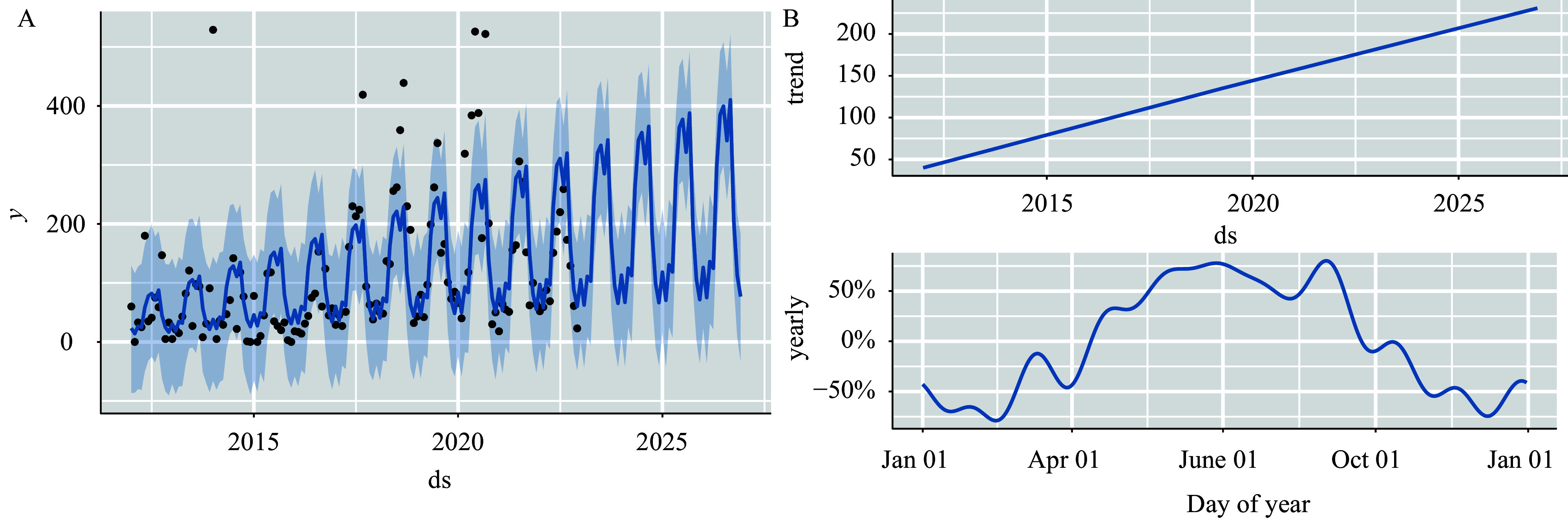
Prophet model projections of the number of incidents of foodborne disease outbreaks in Guizhou Province from 2012 to 2022. (A) The Prophet model prediction plot; (B) the general and seasonal trends of outbreaks.
Figure S2.
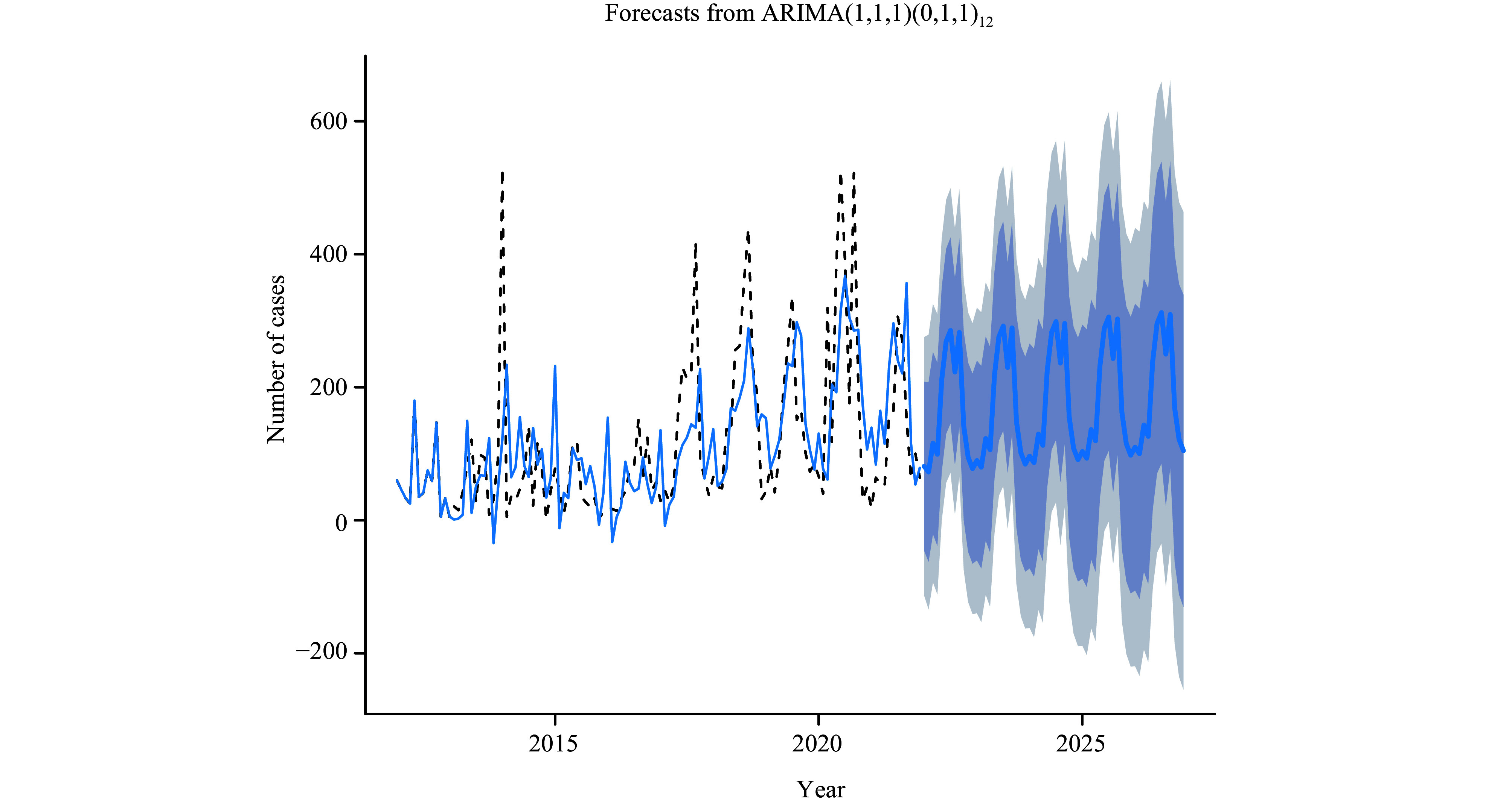
SARIMA model prediction of foodborne disease outbreaks in Guizhou Province from 2012 to 2022.
Abbreviation: SARIMA=seasonal autoregressive integrated moving average.
Figure S3.

ARIMAX (1,1,1) (0,1,1)12 model prediction of the number of incidences of foodborne disease outbreaks in Guizhou Province from 2012 to 2022.
Abbreviation: ARIMAX=multiple difference autoregressive moving average model.
Figure S4.
Optimal model’s trend prediction of the number of foodborne disease outbreaks in Guizhou Province from 2023 to 2025.
SUPPLEMENTARY DATA
Supplementary data to this article can be found online.
References
- 1.Chen W, Xu Y, Lin L. Analysis of foodborne disease outbreaks in Sichuan Province in 2019. Journal of Preventive Medicine Information 2021;37(08):1064−1068, 1074. (In Chinese).
- 2.WHO. WHO estimates of the global burden of foodborne diseases: foodborne diseases burden epidemiology reference group 2007-2015. Geneva: World Health Organization; 2015 Dec. https://www.who.int/publications/i/item/9789241565165.
- 3.Li WW, Pires SM, Liu ZT, Ma XC, Liang JJ, Jiang YY, et al Surveillance of foodborne disease outbreaks in China, 2003–2017. Food Control. 2020;118:107359. doi: 10.1016/j.foodcont.2020.107359. [DOI] [Google Scholar]
- 4.Chen LL, Sun L, Zhang RH, Liao NB, Qi XJ, Chen J Surveillance for foodborne disease outbreaks in Zhejiang Province, China, 2015–2020. BMC Public Health. 2022;22(1):135. doi: 10.1186/s12889-022-12568-4. [DOI] [PMC free article] [PubMed] [Google Scholar]
- 5.Acheson D Iatrogenic high-risk populations and foodborne disease. Infect Dis Clin North Am. 2013;27(3):617–29. doi: 10.1016/j.idc.2013.05.008. [DOI] [PubMed] [Google Scholar]
- 6.Smith B, Fazil A. How will climate change impact microbial foodborne disease in Canada? Can Commun Dis Rep 2019;45(4):108-13. http://dx.doi.org/10.14745/ccdr.v45i04a05.
- 7.Tyagi S, Chandra S, Tyagi G Climate change and its impact on sugarcane production and future forecast in India: a comparison study of univariate and multivariate time series models. Sugar Tech. 2023;25(5):1061–9. doi: 10.1007/s12355-023-01271-2. [DOI] [Google Scholar]
- 8.Wang Y. Time series analysis with R. 2nd ed. Beijing: China Renmin University Press. 2020. https://book.kongfz.com/561989/6738930345/. (In Chinese).
- 9.Mohan S, Solanki AK, Taluja HK, Anuradha, Singh A Predicting the impact of the third wave of COVID-19 in India using hybrid statistical machine learning models: a time series forecasting and sentiment analysis approach. Comput Biol Med, 2022;144:105354. doi: 10.1016/j.compbiomed.2022.105354. [DOI] [PMC free article] [PubMed] [Google Scholar]
- 10.Cheng H, Zhao J, Zhang J, Wang ZY, Liu ZT, Ma XC, et al Attribution analysis of household foodborne disease outbreaks in China, 2010-2020. Foodborne Pathog Dis. 2023;20(8):358–67. doi: 10.1089/FPD.2022.0070. [DOI] [PubMed] [Google Scholar]
- 11.White AE, Tillman AR, Hedberg C, Bruce BB, Batz M, Seys SA, et al Foodborne illness outbreaks reported to national surveillance, United States, 2009-2018. Emerg Infect Dis. 2022;28(6):1117–27. doi: 10.3201/EID2806.211555. [DOI] [PMC free article] [PubMed] [Google Scholar]
- 12.Cissé G Food-borne and water-borne diseases under climate change in low- and middle-income countries: further efforts needed for reducing environmental health exposure risks. Acta Trop. 2019;194:181–8. doi: 10.1016/j.actatropica.2019.03.012. [DOI] [PMC free article] [PubMed] [Google Scholar]
- 13.Kumagai Y, Pires SM, Kubota K, Asakura H Attributing human foodborne diseases to food sources and water in Japan using analysis of outbreak surveillance data. J Food Prot. 2020;83(12):2087–94. doi: 10.4315/JFP-20-151. [DOI] [PubMed] [Google Scholar]
- 14.Xia LL, Qiu S, Wang RT, Li RY, Lyu XH Foodborne disease outbreaks in China from 2011 to 2020. J Hyg Res. 2023;52(2):226–31. doi: 10.19813/j.cnki.weishengyanjiu.2023.02.009. [DOI] [PubMed] [Google Scholar]
- 15.Lake IR, Hooper L, Abdelhamid A, Bentham G, Boxall ABA, Draper A, et al Climate change and food security: health impacts in developed countries. Environ Health Perspect. 2012;120(11):1520–6. doi: 10.1289/ehp.1104424. [DOI] [PMC free article] [PubMed] [Google Scholar]
- 16.Zhan SY. Epidemiology. 7th ed. Beijing: People's Medical Publishing House. 2012. https://book.kongfz.com/27583/4691157030/. (In Chinese).
- 17.Mirón IJ, Linares C, Díaz J. The influence of climate change on food production and food safety. Environ Res 2023;216(Pt 3):114674. http://dx.doi.org/10.1016/J.ENVRES.2022.114674.
Associated Data
This section collects any data citations, data availability statements, or supplementary materials included in this article.
Supplementary Materials
Supplementary data to this article can be found online.