Simultaneous, cortex-wide dynamics of up to 1 million neurons reveal unbounded scaling of dimensionality with neuron number

SUMMARY

The brain’s remarkable properties arise from the collective activity of millions of neurons. Widespread application of dimensionality reduction to multi-neuron recordings implies that neural dynamics can be approximated by low-dimensional “latent” signals reflecting neural computations. However, can such low-dimensional representations truly explain the vast range of brain activity and, if not, what is the appropriate resolution and scale of recording to capture them? Imaging neural activity at cellular resolution and near-simultaneously across mouse cortex, we demonstrate an unbounded scaling of dimensionality with neuron number in populations up to one million neurons. While half of the neural variance is contained within sixteen dimensions correlated with behavior, our discovered scaling of dimensionality corresponds to an ever-increasing number of neuronal ensembles without immediate behavioral or sensory correlates. The activity patterns underlying these higher dimensions are fine-grained and cortex-wide, highlighting that large-scale, cellular-resolution recording is required to uncover the full substrates of neuronal computations.

eTOC BLURB

Neuronal populations have often been argued to exhibit low-dimensional dynamics. Manley et al. record cortex-wide neuronal dynamics and demonstrate that the observed dimensionality is ever-increasing with the number of simultaneously recorded neurons. Most reliable dimensions were distributed cortex-wide, distinct from noise, yet exhibited no correlation with observed sensorimotor variables.

INTRODUCTION

Individual neurons in the brain are not independent processors, but densely interconnected and interdependent units that collectively enable computations underlying the execution of adaptive and goal-directed behavior. It has long been argued that unraveling neural computation will require monitoring the activity of neuronal populations throughout the brain.^1,2 However, until the last decade, recordings were limited to only a few cells simultaneously.^3–5 As a result, some key paradigms have been based on measurable properties of single neurons, and theoretical frameworks for neural computation have aimed to infer how the responses of single cells could arise from the large-scale but unobservable neural circuitry within which they are embedded.^6–10

With the advent of large-scale neuronal recording, it is possible to monitor the activity of larger ensembles of neurons simultaneously^11–29 in behaving animals, in some cases up to the level of whole brains.^30–33 Given the ever-growing number of recorded units, dimensionality reduction has emerged as a powerful tool for visualization and interpretation of neural population dynamics.^34,35 The basic underlying assumption in dimensionality reduction is that the measured variables covary according to a smaller set of “latent” variables which are not measured directly but inferred.

This view has been supported by evidence that under a number of experimental conditions the estimated dimensionality of neural dynamics is much lower than the full state space³⁶ and that relatively few latent signals capture a large proportion of the relevant behavior or stimulus-related activity.^37–39 This redundant coding scheme has been proposed to provide robustness,^9,40–42 yet it can significantly reduce information encoding capacity.^23,43,44 Additionally, the ubiquity of these low-dimensional neural codes suggests that it may be possible to recover the relevant latent dynamics by measuring a subset of neurons.

However, estimates of dimensionality have not always been consistent due to the variety of recording modalities and conditions used across experiments, as well as different definitions of dimensionality.^36,45 In particular, two classes of dimensionality reduction exist that often result in very different estimates of dimensionality. Targeted (or supervised) dimensionality reduction aims to identify neural activity patterns associated with a known task or stimulus, and thus often identifies low-dimensional variables.^46,47 Alternatively, unsupervised dimensionality reduction can infer additional latent signals based on the structure of covariation among neurons,^34,48 and is therefore best suited to quantifying the intrinsic neuronal dimensionality.

Recent studies combining large-scale recording and unsupervised dimensionality reduction suggest that the neuronal dimensionality is higher than previously appreciated. For example, visual cortex contains over 100 latent variables, many of which encode behavior as opposed to solely visual stimuli.⁴⁹ This led to speculation that the dimensionality might continue to grow with the number of neurons,⁴⁹ but quantitative predictions are lacking. In another example, the geometry of visual cortex was shown to be related to stimulus complexity, such that the neural dimensionality is maximized while maintaining robustness and generalization.⁵⁰ High-dimensional representations have also been observed in cognitive tasks,^51–53 where it has been argued that mixed selectivity in neurons increases dimensionality and is critical for cognition.⁵⁴ These results suggest that neural circuits encode as many features as possible, while preserving a correlation structure that balances robustness, efficiency, and flexibility.

Despite increasing evidence for high-dimensional neural geometry, a fundamental question is how the observed neuronal dimensionality would scale with neuron number for any given behavior,⁵⁵ which has only been studied within populations of up to 10,000 neurons.⁴⁹ If the neural dynamics associated with a given task can be truly represented by a low-dimensional system and the neuronal population dynamics are sufficiently sampled, then the measured dimensionality would be expected to exhibit bounded scaling (Figure 1A, orange line). This view, also referred to as the “strong principle” of dimensionality reduction,⁵⁶ would suggest that neural circuits are tuned to encode information redundantly and the experimenter has sufficiently sampled the population. On the other hand, the observation of unbounded scaling, such that dimensionality is ever-increasing with neuron number up to the level of the entire population (Figure 1A, blue line), would suggest that while dimensionality reduction may serve as a useful interpretive technique, the utilized recording technology is still undersampling the population. Importantly, these two scalings imply fundamentally different structural and functional properties of the underlying neural circuitry.

Figure 1. Light Beads Microscopy (LBM) enables large-scale, volumetric recording of neuronal activity across cortex at cellular resolution.

A. A schematic representation of two possible scenarios: bounded versus unbounded scaling of the measured neuronal dimensionality as a function of number of recorded neurons.

B. A schematic of the LBM imaging setup. A 0.5 mm column of light beads is scanned across a lateral FOV with a maximum size of 6 mm (represented by the dashed area on the mouse brain rendering⁹³), enabling volumetric recording of neuronal activity at multi-Hertz rate.

C. The number of recorded neurons is proportional to the size of the imaged volume, ranging from 6,519 to 970,546 neurons.

D. An example single hemisphere recording of 204,798 neurons. Top: the approximate imaging location denoted by a black box. Middle: The standard deviation projection of a plane 183 μm below the cortical surface. Scale bar: 1 mm. Bottom, red inset: zoom in. Scale bar: 100 μm.

E. Z-scored heatmap of neural activity from a 3-minute portion of the single hemisphere recording in panel D. The neurons are sorted utilizing Rastermap.⁹⁴

F. 30 representative examples of individual neuronal traces from the red highlighted region in E.

G and H. Behavior activity corresponding to panels E and F, respectively. The behavior is quantified with total motion energy, defined as the sum of the absolute difference in pixel values between frames.

Here, we hypothesized that observations of low-dimensional neuronal activity were the result of limitations in the recorded population size or in accurately identifying all signal-carrying dimensions. Thus, we systematically investigated how the measured neural dimensionality scales with population size by recording the dynamics of up to one million neurons distributed across mouse dorsal cortex using light beads microscopy²⁴ (LBM) during spontaneous behavior in head-fixed mice. We demonstrated that the measured dimensionality scales according to an unbounded power law with neuron number at least up to one million neurons, suggesting that our technologies are still undersampling the full state space of spontaneous cortical dynamics.

Consistent with previous reports,^49,57–59 we identified a low-dimensional encoding of the animal’s behavior by the ~16 largest dimensions, which accounted for half of the observed neural variance. Each behavior-related signal was encoded by multiple spatially-localized clusters of covarying neurons distributed across both cortical hemispheres, forming a cortex-wide network broadcasting behavioral information.

The remaining higher-dimensional components exhibited no relationship to behavior, a temporal structure distinct from noise, and spanned a continuum of timescales from seconds to the limit of our temporal resolution. Further, this high-dimensional activity was nearly orthogonal to sensory-evoked patterns, suggesting these dimensions underly neural computations lacking an immediate sensory or behavioral correlate. However, the specific function of these signals is unclear. Enabled by the large-scale recording capability of LBM, our results reveal the high-dimensional geometry of spontaneous cortical dynamics and demonstrate that application of low-rank dimensionality reduction to these data would lead to loss of information, as well as systematic biases in the captured spatiotemporal profiles and encoded features.

RESULTS

To investigate the geometry of neuronal population dynamics, we used LBM to image calcium dynamics from up to one million neurons across dorsal cortex (Figure 1B). In LBM, the fluorescent activity of neurons within a 3D field of view (FOV) is captured using a column of 30 axially separated and temporally distinct two-photon excitation spots or “light beads”. These light beads capture neural activity densely along the axial range in rapid succession, providing a spatiotemporally optimal acquisition that is limited only by the fluorescence lifetime of the genetically encoded calcium indicator (GECI). The column of light beads is scanned across the lateral FOV to sample a 3D mesoscopic volume (Video 1). LBM’s versatility allows for an array of recording configurations (Figure S1), yielding populations of 6,519 to 970,546 neurons (Figure 1C). We imaged transgenic mice expressing the GECI GCaMP6s or GCaMP6f⁶⁰ in glutamatergic neurons. An 8 mm cranial window enabled access to most of the dorsal cortical volume, including visual, somatosensory, posterior parietal, retrosplenial, and motor cortices (Figure 1D).

Neural activity across these regions was imaged for one hour while the mouse was free to move on a linear treadmill and exhibited epochs of various spontaneous and uninstructed behaviors (Video 2). Generally, the neural recordings exhibited spatiotemporal activity patterns at multiple scales (Figures 1E-F and S2). Many of these activity patterns were correlated with the animal’s epochs of motor behavior (Figures 1G-H). Together, these neurobehavioral data represent the largest available cellular-resolution recordings of neuronal populations during behavior, providing a unique opportunity to assess the structure of neuronal dynamics.

Reliable dimensionality of cortex-wide neuronal dynamics exhibits unbounded scaling with neuron number

While due to technological limitations it is impossible to estimate the true dimensionality of whole-brain dynamics in the mouse, we aimed to quantify the scaling of the neuronal dimensionality up to the maximum simultaneously observable populations. We hypothesized that the observed dimensionality would only continue to grow as neuron numbers surpassed that of previous recordings. To evaluate this conjecture, we used shared variance component analysis⁴⁹ (SVCA) to identify globally shared components of neuronal covariation.

SVCA first divides the neurons into two subsets (Figure 2A(i)). While other cross-validated dimensionality reduction techniques provide data-driven estimates of dimensionality, SVCA’s utilization of two distinct neural subsets ensures a rigorous degree of self-consistency and eliminates axial crosstalk when interpreting imaging datasets. SVCA identifies the linear dimensions of each neural set’s activity that maximally covary, called the shared variance components (SVCs, see Figure 2A(ii) and STAR Methods). The reliability of each SVC is measured by its covariance between the two neural sets on held-out testing timepoints (Figure 2A(iii)). Compared to traditional dimensionality reduction techniques, this approach allows for a separation between the quality of a latent signal – which is related to its potential biological relevance – and the amount of variance it explains. This is unlike PCA in which some threshold of cumulative variance is generally used to justify the dimensionality of the system. Given that the variance within each component decays smoothly with component number (Figure 2B) and it is difficult to estimate what fraction of the data contains neural signal versus noise, this variance threshold can be an arbitrary decision. Thus, SVCA’s reliability approach provides a data-driven estimate of the latent dimensionality as the number of significantly reliable SVCs compared to a noise floor or shuffling test.

Figure 2. Shared variance component analysis (SVCA) reveals unbounded scaling of reliable neural dimensionality.

A. Schematics of SVCA: (i): SVCA splits the neurons into two sets (green and purple). (ii): SVCs are the maximally covarying projections of each neural set. (iii): The reliability of each neural SVC is quantified using the covariance of the two sets’ projections on held-out testing timepoints.

B. The normalized variance spectra across neural SVC dimensions decays smoothly. Data from a 3×5×0.5 mm³ single hemisphere containing 146,741 total neurons.

C. The percentage of reliable variance quantifies the robustness of each SVC, which eventually decreases at higher SVCs. The data for the same population as in panel B is shown in black. The shuffled data is shown in red, where the neural sets were drawn from distinct recordings.

D. Visualization of the reliability of SVCs as a function of neuronal population size. SVC signals for both neural sets from a random sampling of (i): 1,024 and (ii): 970,546 total neurons from a 5.4×6.0×0.5 mm³ bi-hemispheric recording. The percentage of reliable variance in each SVC is shown on the left.

E. The reliable dimensionality grows with neuron number. Colored traces show different size neural populations randomly sampled from the population in panel D, with each trace indicating the mean percentage of reliable variance in each SVC over n=10 samplings.

F and G. The reliable dimensionality exhibits unbounded scaling with neuron number across different neuronal sampling strategies. The reliable dimensionality represents the number of SVCs a reliability greater than four standard deviations above the mean of shuffled data. Each line indicates the mean over n=10 samplings in a single recording. In F, neurons are sampled randomly from the entire volume, while in G, neurons are sampled in order of their distance from the center of the volume.

Applying SVCA to a cortical hemisphere recording containing 146,741 neurons, we found that 486 ± 33 dimensions exhibited greater reliability than shuffled data (mean ± 95% confidence interval (CI) across n=10 random samplings, Figure 2C). To quantify how the number of reliable SVCs behaved as a function of the number of sampled neurons, we performed SVCA on various subsets of neurons sampled randomly from across the imaging volume. As expected, many more components exhibited strong covariation as the number of sampled neurons increased (Figures 2D and S3A-B). For example, while small populations of only 256 neurons contained 11 ± 6 reliable dimensions, our largest sampling of 970,546 neurons contained 2,300 ± 38 dimensions with greater reliability than in shuffled data (Figure 2E). This increase in reliability with the number of sampled neurons what was not found in shuffled data (Figure S3C). Further, such shuffled datasets only contained 6.4 ± 2.8% total reliable variance across all SVCs (Figure S3D), as compared to the 63.1 ± 11.0% reliable variance observed in the original data (mean ± 95% CI across n=12 recordings, significantly different from shuffled datasets with p<0.001, two-sided t-test). This analysis revealed an unbounded power law scaling of reliable dimensionality with the number of sampled neurons (Figure 2F) at least up to the maximal recorded population size of a million neurons, with a power law exponent of $\alpha =0.66\pm 0.06$ (mean ± 95% CI across n=12 recordings). Moreover, this unbounded scaling of reliable dimensionality was consistent across other arbitrary choices for a minimum reliable variance threshold (Figure S3E).

To demonstrate that this observed unbounded scaling was not due to physiological confounds such as hemodynamic effects⁶¹ or uncorrected sample motion artifacts, we imaged mice with broad neuronal expression of green fluorescent protein (GFP), a static fluorescent reporter. Few reliable SVCs were detected within GFP data (Figure S3F) compared to the hundreds of reliable SVCs identified from GCaMP-expressing animals. Importantly, only 2.1 ± 0.2% of the total GFP variance was reliable (Figure S3G), as compared to 63.1 ± 11.0% total reliable variance within the GCaMP recordings (mean ± 95% CI across recordings, significantly different with p<0.001, two-sided t-test).

These data highlight the high-dimensional geometry of spontaneous cortical dynamics and suggest that the ability to infer higher-dimensional neuronal dynamics will only continue to improve with increasing recording capacity. In fact, these estimates likely represent only a lower bound on the true dimensionality of the cortical population activity given that we are sampling at most ~10% of cortical neurons. Moreover, we demonstrated that the measured reliable dimensionality depended on the imaging rate and duration (Figures S4A-B). Finally, any neuronal dynamics faster than the GCaMP response kernel are likely attenuated, further reducing the observed neural dimensionality.

Notably, the unbounded scaling of the reliable dimensionality of the neural population activity highlights the limitation of traditional variance-based approaches. The variance spectra as a function of SVC dimension exhibited only minor changes with neuron number (Figure S4C), suggesting that the amount of variance within each SVC does not necessarily correlate with its reliability. Accordingly, the number of principal components (PCs) required to explain some percentage of the total variance exhibited bounded scaling with neuron number (Figure S4D). While a component may explain only a small fraction of the variance, it can still contain reliable information if the number of sampled neurons is sufficiently large.

Finally, given that the above observations were based on random sampling from across the imaged volume, we asked whether our observed scaling of reliable dimensionality depended on the spatial sampling pattern. Interestingly, the scaling law was independent of the sampling strategy; sampling from an expanding FOV exhibited a consistent power law exponent of $\alpha =0.75\pm 0.08$ (Figure 2G), not significantly different from random sampling (p=0.10, two-sided t-test). We further corroborated this observation by confirming that this scaling was also conserved for different sampling densities (Figure S4E).

The above observations demonstrate that the dimensionality of spontaneous cortical dynamics is primarily dependent on the recorded neuron number as opposed to their spatial distribution across the volume or among cortical regions, implying the latent SVCs are widely distributed across cortex. This unbounded power law scaling up to the maximal observed population size was consistent across recordings, experimental configurations, and sampling strategies, demonstrating that the cortex indeed encodes a very high-dimensional set of latent signals which cannot be identified without simultaneous observation of the activity of very large numbers of neurons.

The majority of reliable neural dimensions lack an immediate behavioral or sensory correlate

Linking such inferred latent dimensions to sensory inputs, motor actions, and cognitive processes is key to understanding neural computations. Thus, we next investigated how behavior-related information is distributed across the neural SVCs. Specifically, we asked whether the unbounded scaling of the reliable dimensionality of cortical dynamics represents an increase in the number of encoded behavior-related features or an increase in signals that lack an immediate motor or sensory correlate. Such neural signals without immediate external correlates could underly neuronal computations, internal states such as motivational drives,^62,63 or diverse modes of information processing.^39,64

To differentiate these two alternatives, we captured the animals’ spontaneous and uninstructed epochs of behavior using a high-speed camera (Figure 3A). We quantified each mouse’s behavior by computing the PCs of facial motion energy (Figure 3B, see STAR Methods), referred to as behavior PCs. The observed behavior appeared multi-dimensional across mice and imaging sessions (Figure S5A), with 256 PCs explaining 92 ± 3% of the captured motion energy variance. Additionally, the behavior PC activity clustered according to various behavioral motifs (Figures S5B-C), providing a useful moment-to-moment description of spontaneous behavior.

Figure 3. Behavior-related activity is encoded in a low-dimensional subspace of reliable neuronal dynamics.

A. Example behavior videography image, with a box denoting the area in which facial motion energy was monitored.

B. The top three behavior PCs for an example mouse.

C. Schematics of the prediction of neural SVCs from the behavior PCs. SVCs are predicted from behavior PCs using either a linear or nonlinear (multilayer perceptron, MLP) regressor. While all models predict a single timepoint of neural SVC activity, the behavior PC inputs are either: instantaneous or multi-timepoint.

D. Example z-scored SVC timeseries (green) and their linear, instantaneous predictions from behavior PCs (purple) using held-out testing timepoints. While the initial SVCs appear highly predictable from behavior, the higher SVCs (e.g., SVC 64) do not. Scalebars at the right visualize the relative scale of each SVC.

E. Only the lowest neural SVCs are predictable from instantaneous behavior. Using the linear, instantaneous reduced-rank regression model, the percentage of each SVC’s reliable variance that is explained by behavior decays rapidly with SVC dimension, such that only 16 ± 8 SVCs (mean ± 95% CI, n=6 recordings with at least 131,072 neurons) show significantly more variance explained by behavior than shuffled data (indicated in red, p<0.05, two-sided t-test). Each line indicates one recording.

F. Saturation of predictability of neural SVCs from behavior with increasing neuron number. Using the linear, instantaneous model, the reliable variance explained by behavior saturates around 10,000 neurons in the first 32 SVCs (individual recordings in gray). The remaining SVCs above 32 (orange) are not predictable from behavior at any neuron number.

G. The lowest, behavior-related SVCs represent a much greater fraction of the neural variance during epochs of motor behavior. Timepoints were separated into idle and motor epochs (see STAR Methods). The ratio of the fraction of variance explained by each SVC during behaving versus idle epochs is shown. Shown in panels G-I is the mean ± SEM of n=6 recordings with at least 131,072 neurons.

H. A comparison of the three different model types: linear, instantaneous; nonlinear (MLP), instantaneous; and linear, multi-timepoint. Including nonlinearities and history both slightly improve the prediction of the first neural 32 SVCs.

I. Each neural SVC’s percent reliable variance explained by behavior for the three models. The SVCs for each recording are sorted by the percent of their reliable variance that is explained by behavior. Multi-timepoint models (gray line) predict many more SVCs than the instantaneous models (black and blue lines). The shuffled data for the linear, multi-timepoint models are shown in red. The lines of corresponding color at the top of the plot indicate the number of SVCs that exhibit significantly higher predictability than shuffled data (p<0.05, two-sided t-test).

J. Volumetric neural activity patterns and corresponding predictions from behavior. (i) Instantaneous facial motion energy. (ii-iv) Example coarse-grained volumetric neural activity maps (ii), predictions from behavior using a linear, multi-timepoint model (iii), and their difference (iv). Timepoint t₁ occurs during grooming, whereas t₂ is idle. Shown is an example 5×6×0.5 mm³ bi-hemispheric recording. The scale bars in (ii) correspond to 1 mm laterally and 250 μm axially.

To infer the behavior-related versus non-behavior-related activity encoded by the neural SVCs, we utilized linear and instantaneous reduced-rank regression to predict SVCs from the first 256 behavior PCs (see STAR Methods). This approach allowed us to quantify what fraction of the reliable variance in each SVC was behavior-related (Figure 3C). While the lowest SVCs were highly predictable from behavior PCs, the higher SVCs did not appear as predictable (Figure 3D). This was consistent across mice (Figure 3E), with only 16 ± 8 SVCs exhibiting significantly greater predictability from behavior than shuffled data (mean ± 95% CI, p<0.05, two-sided t-test).

We next asked how the fidelity of behavior-related encoding depended on the number of sampled neurons. The percentage of reliable variance in the first 32 neural SVCs explained by behavior initially increased with the number of randomly sampled neurons, but saturated on the order of 10,000 neurons (Figure 3F, gray lines). This is consistent with our previous observation that the first 32 SVCs were highly reliable in populations of 10,000 or more neurons, given that on average the first 87 ± 23 SVCs exhibited >75% reliable variance (mean ± 95% CI across n=10 recordings, Figures 2E and S3E). In contrast, the remaining higher reliable SVCs were not predictable from behavior irrespective of the number of recorded neurons (Figure 3F, orange lines). Additionally, we confirmed that behavior PCs could not predict any of the neural SVCs extracted from our static GFP recordings (Figure S5D), demonstrating that our ability to predict GCaMP dynamics from behavior was not due to uncorrected motion-induced artifacts or other confounds. Thus, while a significant fraction of observed cortical activity is correlated with immediate behavior, the majority of reliable neural SVCs were not related to animals’ immediate behavior. Indeed, the observed high-dimensional neuronal geometry persisted in idle epochs when the animal was not engaging in any motor behavior; however, the neural variance was more concentrated in the first 16 SVCs during motor behavior (Figure 3G).

To corroborate this conclusion, we further tested whether our inability to predict higher order SVCs from behavior was due to the simplicity of the linear, instantaneous model. Thus, we investigated whether utilizing a nonlinear or multi-timepoint model would result in an increase in predictability of the higher neural SVCs from behavior (see STAR Methods). While all such improvements could increase the percentage of reliable neural SVC variance explained by the behavior PCs (Figure 3H), only the multi-timepoint models were able to predict significantly more additional neural SVCs on average (Figure 3I, 129 ± 54 SVCs, mean ± 95% CI) than shuffled data (p<0.05, two-sided t-test; see also Figures S5E-F). The average predictability from behavior was optimal for a window from 6 seconds before to 3 seconds after the instantaneous neural activity (Figure S5G). To confirm that these additional higher neural SVCs indeed encode an integration of the recent behavior, we showed that they could not be predicted by finding an optimal lag for each of the SVCs individually (Figure S5H), as opposed to the common lag utilized in the linear, instantaneous model.

We then visualized the predictions of these neural SVCs from behavior by transforming the predicted SVCs back into the neural space and plotting their volumetric activity maps (Figure 3J and Video 3, see STAR Methods). Agreement between the coarse-grained neuronal activity patterns and those predicted from the behavior PCs was high during epochs of spontaneous behavior (Figure 3J(ii-iv), top row t₁). In contrast, the prediction fidelity was highly reduced for idle epochs (Figure 3J(ii-iv), bottom row t₂), further indicating that a significant fraction of the variance across neural SVCs represents activity not immediately related to behavior.

We next asked whether additional behavioral features that might have not been captured by the single camera view could predict any remaining neural activity. To comprehensively quantify the animals’ behavior, we combined an all-around multi-camera behavior rig with more interpretable behavioral features identified using posture keypoint tracking with DeepLabCut.⁶⁵ Three cameras were pointed at the animal from different perspectives (Figure 4A) allowing simultaneous tracking of (1) the mouse’s pupil, facial expression, and whiskers; (2) the other side of the animal’s face, front limbs, and torso; and (3) all four of the limbs and the tail from below using a transparent wheel.⁶⁶

Figure 4. Lack of correlation of high-dimensional neural SVCs with comprehensive behavioral monitoring and sensory-related activity.

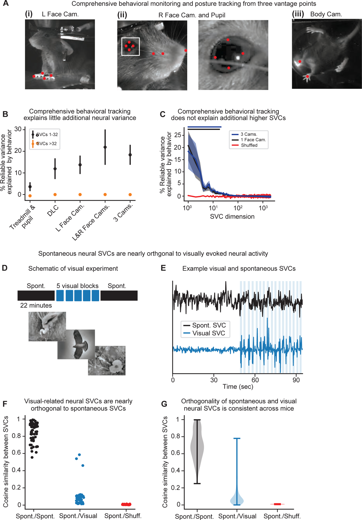
A. Example images from simultaneous, all-around behavior monitoring. (i) The left side of mouse. (ii) Left: the right side of the face and pupil. Right: an inset depicting the pupil. (iii) The body of the mouse from underneath, which can freely move on a transparent wheel. Shown as red dots are tracked keypoints.

B. Interpretable behavior features and comprehensive behavioral monitoring explained little additional neural variance. Shown is the percentage of reliable neural variance explained by behavior within the first 32 SVCs (black) compared to the higher SVCs (>32, orange) as a function of the complexity of the behavioral tracking (mean ± 95% CI across n=6 recordings). Treadmill: the mouse’s running speed measured via the treadmill; pupil: pupil diameter; DLC: speeds of all tracked keypoints; cameras: corresponding to labels in A.

C. Additional behavior features did not explain significantly more neural SVCs. Shown is the percentage of reliable variance within each neural SVC that is explained by behavior utilizing a single camera (black) as in Figure 3, compared to all three cameras (blue, mean ± SEM of n=6 recordings). The lines of corresponding color at the top of the plot indicate the number of SVCs that exhibit significantly higher predictability than the shuffled data (p<0.05, two-sided t-test).

D. Schematic of the visual stimulation experiments (see STAR Methods). Three example natural images are shown.

E. Timeseries of example SVCs identified from spontaneous (black) or trial-averaged visual (blue) neural activity. The timing of visual stimulus presentations is highlighted in blue. While visual components were highly synchronized to the visual stimulation, spontaneous SVCs did not show stimulus-locked activity patterns.

F. Visually-related SVCs are nearly orthogonal to spontaneous SVCs. Shown for a single recording is the distribution of maximum cosine similarity between the spontaneous SVCs and those identified during either another spontaneous epoch (Spont./Spont., black), the visual stimulation epoch (Spont./Vis., blue), or shuffled data (Spont./Shuff., red). Values of 1 indicate identical neural representations, whereas 0 indicates orthogonal and independent representations.

G. Orthogonality of spontaneous and visual SVCs across mice. As in panel F, except across n=4 recordings. The Spont./Spont. cosine similarities (black) are significantly higher (p<10⁻⁶, two-sided Wilcoxon rank-sum test) than Spont./Visual (blue). The Spont./Visual cosine similarities are significantly higher (p<10⁻⁶, two-sided Wilcoxon rank-sum test) than the Spont./Shuff. (red).

Using these data, we asked whether any additional neural SVCs could be explained by comprehensive behavioral monitoring (Figure 4A). While simpler metrics such as the treadmill speed or pupil diameter explained only a minor fraction of the variance within the first 32 neural SVCs, higher variance was explained by the camera views (individually or combined, Figure 4B), consistent with previous reports.⁴⁹ However, while utilizing the comprehensive behavioral tracking did allow for a moderate increase of the variance explained in the lower SVCs (<32), this was not the case for the higher SVCs >32 (Figure 4B). Thus, including additional camera views did not explain a significantly greater number of neural SVCs (Figure 4C), with 18 ± 10 SVCs (mean ± 95% CI) significantly explained by a single face camera compared to 21 ± 12 SVCs utilizing three cameras (p=0.30, paired t-test).

Finally, we tested whether the higher neural SVCs could be explained by external sensory variables. While all recordings were conducted within a sensory-blocking enclosure to significantly dampen any external time-varying sensory inputs, we nonetheless performed visual stimulation experiments to explicitly compare the representation of such sensory-related information to neuronal activity patterns during spontaneous behavior. Thus, while performing volumetric cortex-wide LBM recordings we presented 180 distinct visual stimuli (Figure 4D, see STAR Methods).

We then applied SVCA to trial-averaged visual responses (see STAR Methods), resulting in a set of visually-driven SVCs which could be compared to spontaneous SVCs computed when visual stimuli were not presented (see example timeseries in Figure 4E). To quantify any overlap between visual and spontaneous SVCs, we quantified the maximum cosine similarity between the neuronal coefficient vectors ${\stackrel{\rightharpoonup }{u}}_k$ from visual SVCs versus spontaneous SVCs. This cosine similarity is 1 if the neuronal activity patterns described by the pair of SVCs are perfectly aligned across the epochs, and 0 if they are orthogonal. The cosine similarity between visual and spontaneous SVCs was significantly lower than those between the SVCs identified during two spontaneous epochs (Figure 4F-G), demonstrating that the visually-driven dimensions are nearly orthogonal to those identified during spontaneous behavior. This is consistent with previous results demonstrating orthogonality between spontaneous and visually-driven neural activity patterns except along a very low-rank shared visual-behavior subspace,⁴⁹ which results in outliers seen within the Spont./Visual distribution (Figure 4F).

In summary, we confirmed that the comprehensive behavior-related information was encoded by relatively few (~16 to 21) neural SVCs which accounted for only half of the total neural variance (54 ± 12% of total variance, mean ± 95% CI of n=12 recordings). Additionally, almost all SVCs were nearly orthogonal to sensory representations. This means that more than half of the observed reliable variance in these lower dimensions, as well as all the observed reliable variance in the remaining higher SVCs, carry information that is partially hidden and lacks an immediate behavioral or sensory readout.

Reliable neural SVCs exhibit a continuum of timescales and spatial distributions

eural computations are carried out by the spatiotemporal dynamics of populations of neurons distributed across brain regions. While the function of the observed higher SVCs is not immediately clear, we next investigated whether these dynamics exhibited characteristic spatiotemporal scales that may provide insight into the computations they could perform.

First, we asked if the neural SVC dynamics exhibited a characteristic timescale. We fit an exponential decay to each SVC’s autocorrelation, thus defining its dominant timescale τ. While an SVC may exhibit dynamics across multiple timescales, our approach captures the single most dominant timescale within each SVC’s autocorrelation. The dominant timescales spanned a wide range from minutes to hundreds of milliseconds (Figures 5A and S6A), which was not observed in temporally shuffled data (Figure S6B). The measured dominant autocorrelation timescale decayed with neural SVC number in all recordings (Figure 5B). The lower, behavior-related SVCs had the longest dominant timescales, on the order of seconds to hundreds of seconds, whereas the higher SVCs operated at timescales of seconds or less, down to the minimal observable timescale in our data. The observed power and reliable variance in the fastest timescales is likely attenuated by the GCaMP response kernel (i.e. <550 ms⁶⁷) and in some cases the imaging rate, whereas 50.8 ± 14.4% of reliable SVCs (mean ± 95% CI across n=12 recordings) with a response time >550 ms are not attenuated by the GCaMP response or imaging speed.

Figure 5. Latent neural SVC dynamics represent a continuum of timescales.

A. Example autocorrelation curves for four neural SVCs from the same recording as Figure 2B-C.

B. Characteristic dominant timescales within each SVC. The dominant autocorrelation timescale τ, computed by fitting an exponential decay to the autocorrelation, decays with neural SVC dimension. Gray lines show n=6 recordings with at least 131,072 neurons, black indicates their mean. Shown are SVCs with at least 25% reliable variance on average.

C. Characteristic dominant timescales increase as a function of the number of recorded neurons. As in B, but with a varying number of randomly sampled neurons. Shown is the mean dominant timescales across recordings, with each neuron number randomly sampled four times per recording.

D - G. Example heatmaps of reconstructed neural activity from various SVCs for the recording in Figure 1E. D. Reconstructed activity from SVCs 1–15. E. Reconstructed neural activity from SVCs 16–256, which visually exhibits shorter timescale dynamics and a greater diversity of neuronal coactivation patterns. F and G display the red highlighted insets in D and E, respectively.

H and I. Corresponding timeseries for example SVCs used in D and E, respectively.

As the number of sampled neurons increased and more SVCs became reliable, the number of SVCs with functional timescales greater than the sampling period also increased (Figure 5C). Thus, not only were these higher SVCs statistically reliable as defined previously, but they displayed a continuum of dominant timescales from the limit of our detection up to the order of seconds. The reliable activity patterns encoding these dominant timescales could further be visualized by reconstructing the full neural activity from a low-rank approximation utilizing various numbers of SVCs (Video 4). While the first 15 SVCs indeed exhibited longer timescale patterns of coactivation across many neurons (Figures 5D, F, and H), the higher order SVCs contained many more finer timescales and patterns of neural activity (Figures 5E, G, and I).

The characteristic decay of dominant timescales observed within our neural SVCs is highly consistent with the 1/f nature of power spectra of neural activity observed across experimental paradigms and species,^68,69 commonly measured via the sum of many thousands of neurons’ activities in electroencephalography or local field potentials. Indeed, the SVCs exhibited a 1/f-like power spectrum as a function of their dominant timescales (Figure S6C). Thus, these data provide an opportunity to evaluate how dynamic activity patterns that have a known biological function may be executed at the mechanistic level across scales, from the level of single neurons to brain-wide distributed networks.

Finally, the cortex-wide FOV of LBM enabled us to examine the spatial extent of the SVCs by identifying neurons which contributed significantly to each SVC, which we term “participating” (see STAR Methods). In an example cortical hemisphere recording, the neurons participating in the lowest SVCs appeared hemisphere-wide yet spatially clustered, characterized by multiple apparent clusters on the order of hundreds of microns distributed across many cortical regions (Figure 6A(i-ii)). The spatial distribution of neurons contributing to the higher reliable SVCs, on the other hand, appeared much more uniformly distributed across the imaging volume (Figures 6A(iii-iv) and S6D, Video 5). We quantified these spatial patterns by computing a local homogeneity index, which measured the average percent of neighbors within a given distance of a participating neuron which were also participating in that same neural SVC. The local homogeneity confirmed that the behavior-related SVCs exhibited spatial clustering that decayed with distance, while the higher SVCs in some cases showed no local clustering (Figure 6B). We found similar patterns of local homogeneity in our bi-hemispheric recordings (Figures 6C-D and S6E, Video 6), which showed that nearly all SVCs were distributed in a cortex-wide fashion. The particular spatial patterns observed in each SVC varied across recordings due to inherent differences in the observed FOVs and because physiologically-similar SVCs are not expected to maintain a consistent variance-ranked order across recordings. However, the local homogeneity was consistent across mice, with the first nearly 100 SVCs exhibiting some degree of local homogeneity, whereas shuffled data exhibited no spatial structure (Figure 6E). Lastly, we quantified the number of neurons contributing to each SVC across recordings and found that the lowest, spatially-clustered components exhibited the largest participation (Figure 6F), followed by a slow decay with SVC dimension. Together, these spatial profiles make up a diverse repertoire of cortex-wide functional connectivity patterns which have been resolved at single neuron resolution for the first time. This combination of a continuum of timescales and a diversity of cortex-wide spatial patterns represents a broadly-distributed network that may underly the transmission and manipulation of information throughout the cortex in order to enable the various computations and adaptive behaviors produced by the mammalian brain.

Figure 6. Lower and higher neural SVCs form distinct, spatially organized neuronal assemblies.

A. Lower and higher SVCs exhibit distinct cortex-wide neuronal distribution profiles. The lateral spatial distribution of the neurons participating in four example SVCs in a single hemisphere recording containing 315,363 neurons. Scale bar, 1 mm.

B. The local homogeneity, which quantities local spatial clustering of participating neurons, decreases with SVC number. The local homogeneity index, computed as the average percent of neighbors within a given distance that are also contributing to that same neural SVC, as a function of the radial distance for the four example SVCs in A.

C. The spatial distribution of the participating neurons contributing to four example SVCs in a bi-hemispheric recording with 970,546 neurons. The neurons contributing to each SVC are generally not restricted to single cortical regions or hemispheres. Scale bar, 1 mm. See also Video 6.

D. The local homogeneity index as a function of distance shown for the SVCs in panel C.

E. The local homogeneity index profiles are consistent across mice. The local homogeneity computed at a radial distance of 30 μm for n=6 recordings. Each recording is shown in gray and their mean is showed in black. The mean of n=6 shuffled recordings is shown in red.

F. Hundreds of neurons participate in each neural SVC. Shown is the mean ± 95% CI of the number of participating neurons for each SVC dimension across n=6 recordings (black), compared with shuffled datasets (red).

DISCUSSION

While technological advancements over the last decade have pushed the number of simultaneously recorded neurons by several orders of magnitude across species, the emerging notion is that the relevant dynamics of neuronal dynamics are confined to low-dimensional manifolds that reflect neural computation, particularly the encoding of stimuli^70–74 and behavioral states.^38,75–77 If true, this would beg the question of the biological utility of such a highly redundant and metabolically costly encoding scheme, and would raise the question to what extent technological advances aimed at further increasing the number of recorded neurons would be necessary.

We hypothesized that in many cases the observed low-dimensional neural encoding is a reflection of technological limitations, ad hoc choices in dimensionality reduction analysis, or a focus on only a subset of the population dynamics. LBM’s unique capability allowed us to test the conjecture that the measured neuronal dimensionality would continue to grow as a function of the size of sampled neuronal population. In all cases, the reliable dimensionality was 100 to 1000-fold lower than the number of neurons, indicating that dimensionality reduction is still highly appropriate. However, we demonstrate for the first time that the reliable dimensionality scales in an unbounded fashion and according to a power law with the number of neurons, at least up populations of one million neurons, with additional latent components expected at higher neuron counts. However, it is still unclear at what scale of recording the observed linear dimensionality may saturate. Whilst our data solidify the notion that neural activity is high-dimensional, it also shows that the two viewpoints – that of low- and high-dimensional findings within neuronal dynamics – are not mutually exclusive, but dependent upon the analytical framework and the recording modality at hand.

By establishing the relationship between the reliable neural SVCs and the animal’s epochs of spontaneous behavior, we identified a low-dimensional encoding of spontaneous behavior within 16 ± 8 of the largest neural dimensions. While this observation is consistent with recent studies that have shown a broad representation of motor behavior across the brain,⁷⁸ our work extends this finding in several ways. First, our systematic study of scaling, combined with a 1000-fold increase in neuron count relative to the previous largest experiments,²² provides strong evidence that this low number of behavior-related dimensions is a cortex-wide property. Second, each behavior-related dimension was encoded by multiple spatial clusters of neurons across cortex, likely representing a structured brain-wide network broadcasting the behavioral state of the animal. Finally, the low-dimensional encoding of behavior and nearly orthogonal encoding of sensory activity demonstrated that the largest gains from large-scale recordings come from the ability to robustly infer signals without a time-locked behavioral or sensory correlate, which we speculate could encode purely internal signals involved in neuronal computations. In total, we found that >90% of the reliable neural dimensions showed no temporal correspondence with the epochs of spontaneous motor behavior. Taken together, our results demonstrate that hundreds of reliable higher neural dimensions cannot be explained by physiological confounds, the animal’s immediate behavior, or its sensory environment. However, additional work is required to link such dynamics to specific biological functions.

Importantly, while the variance in our detected reliable SVCs decays with SVC number, the higher neuronal dimensions cannot be disregarded due to their magnitude, as they collectively still represent levels of activity known to influence neural function. Collectively, SVCs >100 contained 3.5 ± 0.2% of the reliable neural variance (mean ± 95% CI across n=10 samplings) of the 970,546-neuron shown in Figure S3C. Further, the smallest reliable dimensions exhibit a normalized reliable variance greater than 10⁻⁶ and thus contribute at least on the order of a single neuron’s activity which as we argue should not be ignored due to the sheer size of the recorded neuronal population. Further, while neuronal dynamics are the product of a highly interconnected population of neurons, the activity of a single neuron has been shown to be able to affect the population response,⁷⁹ as well as trigger detectable changes in behavior.⁸⁰ Regardless, recent work in a memory-guided decision-making task demonstrated that low variance dimensions can indeed have a significant behavioral influence due to amplifying feedforward connectivity.⁸¹ Importantly, this finding is in contrast to the common assumption in neural dimensionality reduction that the largest amplitude signals have the largest influence on behavior.

Thus, while our LBM data add to the growing evidence that the encoding of behavior occurs in a broadcasted manner that may facilitate the integration of sensory and motor variables as early as primary sensory cortex, we speculate that the higher SVCs may underlie a similar brain-wide network which broadcasts purely internal signals, such as attention, motivation, hunger or thirst, and fear. These variables often primarily serve to modulate the ways in which neural circuits, and thus the animal’s behavior, respond in a dynamic and adaptive fashion to an ever-changing sensory environment, and thus may need to be combined with sensory, motor, and other signals that are encoded and manipulated across the entire brain. We expect that the combination of large-scale recording technologies with ethologically-relevant tasks and data-driven quantification of behavior provide a promising avenue to understand how potential internal variables are combined with sensory and motor representations to shape behavior across trials and over a lifetime.

Additionally, the various temporal and spatial scales at which the SVCs operate provide evidence for the multi-scale and potentially hierarchical nature of neural activity. Early work attempted to quantify spatiotemporal relationships between single neurons and the activity in their surrounding environment and it was hypothesized that spatially distributed and correlated neural activity could aid in context-dependent processing in the brain.⁸² More recently, it has been shown that the spatial distribution of cortical activity can vary significantly depending on the type of computation employed and that increased cognitive demand is associated with a more widespread engagement of neural activity across cortex.⁸³ However, such results have previously only been possible at this scale utilizing widefield calcium recordings lacking cellular resolution. At the same time, the temporal structure and characteristic 1/f-like power spectra within neural activity have been shown to be modulated by various processes such as sensory stimulation⁸⁴ and task performance,⁸⁵ suggesting that the observed diversity of timescales of neural activity are functionally significant. Taken together, our data highlight the potential hierarchical scales of activity spanned by cortical dynamics and provide a unique starting point to investigate how brain-wide phenomena and adaptive behavior arise from the interaction of individual spiking neurons.

Finally, we note that the techniques implemented here provide a data-driven estimate of the linear dimensionality, and a more general estimation of the intrinsic dimensionality of complex systems has proven challenging.^86–88 For instance, the relationship between latent dimensionality and neural population size is expected to also be a function of the complexity of the animal’s environment and tasks,⁸⁹ and we have focused on spontaneous dynamics while the animals were isolated and in the dark. Additionally, although by far the most common approach, quantifying the linear dimensionality does not account for the possibility that the intrinsic dimensionality of cortical dynamics may be lower if it lies on a highly nonlinear manifold. However, nonlinear manifold inference is computationally challenging and often requires assuming a simple topological structure.^34,90,91 Nonetheless, the linear dimensionality has been argued to be important for how information is processed by neural circuits,⁴⁸ particularly given the wealth of evidence suggesting that sensorimotor and cognitive systems actively create representations that enable linear decodability.^53,90,92 We expect that advancements will be made towards a more systematic inference of nonlinear manifolds and that the development and validation of these tools would benefit from large-scale recording capabilities.

STAR METHODS

RESOURCE AVAILABILITY

Lead contact

Further information and requests for resources should be directed to the lead contact, Alipasha Vaziri (vaziri@rockefeller.edu).

Materials availability

This study did not generate new unique reagents.

Data and code availability

The codebase used to perform these analyses is available at https://github.com/vazirilab/scaling_analysis. This codebase and example processed datasets are deposited at https://doi.org/10.5281/zenodo.10403684. All other information required to reanalyze the data reported in this paper is available from the lead contact upon reasonable request.

EXPERIMENTAL MODEL AND SUBJECT DETAILS

Animal subjects

Transgenic mice expressing either GCaMP6s or GCaMP6f in glutamatergic neurons (Ai162D or Ai148D x Vglut1-IRES2-Cre-D, Jackson Labs stock numbers 031562, 030328, and 037512 respectively⁶⁰) and wild-type (C57BL/6J) mice were bred in house. Male and female mice were studied, and any effect of sex was not investigated. All mice were 30–95 days of age at the time of first procedure and were 47–170 days old during imaging experiments. Mice were allowed food and water ad libitum.

METHODS DETAILS

Surgical procedures

All surgical and experimental procedures were approved by the Institutional Animal Care and Use Committee of The Rockefeller University. Cranial window implantation was performed as previously described.²⁴ During implantation, mice were anesthetized with isoflurane (1–1.5% maintenance at a flow rate of 0.7–0.9 L/min) and placed in a stereotaxic frame (RWD Life Science). The scalp and underlying connective tissue were removed and cleared from the skull. A custom stainless-steel head bar was fixed behind the occipital bone with cyanoacrylate glue (Loctite) and covered with black dental cement (Ortho-Jet, Lang Dental). A circular 8 mm diameter dual-hemisphere craniotomy was performed, leaving the dura intact. An approximately 1 mm segment of skull at the furthest posterior bound of the diameter of the craniotomy was left intact to avoid the junction of the sagittal and transverse sinus vessels while drilling. The cranial window was formed by implanting a circular 8 mm glass coverslip with 1 mm of the bottom removed (#1 thickness, Warner instruments) before sealing with tissue adhesive (Vetbond). The remaining exposed skull around the cranial window was covered with cyanoacrylate glue and then dental cement. Post-operative care included 2 days of subcutaneous delivery of dexamethasone (2 mg/kg), 3 days of subcutaneous delivery of meloxicam (0.125 mg/kg), and antibiotic-containing feed (LabDiet no. 58T7). After surgery, animals were returned to their home cages and were given at least one week to recover before imaging experiments. Mice with damaged dura, significant regrowth or otherwise unclear windows were euthanized and not used for imaging experiments.

In the case of static GFP imaging experiments in Figures S3D and S3F-G, brain-wide expression of genetically encoded green fluorescent protein (GFP) was achieved by retro-orbital injection of 100 μL of AAV-PHP.eB CAG-GFP (2.7 * 10^12 vg/mL) into wild-type (C57BL/6J) mice. Animals were injected one week after implantation of the cranial window.

Imaging parameters

Data acquisition was performed utilizing LBM as previously described,²⁴ utilizing a custom multiplexing module interfaced with a commercial mesoscope (Thorlabs, Multiphoton Mesoscope). n=11 total mice, male or female, were imaged across n=25 sessions for a duration of 30 minutes (n=2), 60 minutes (n=13), 90 minutes (n=6), or 120 minutes (n=4). Three FOV types were recorded: 1.2×1.2×0.5 mm³, 2 μm lateral pixel spacing, at 10 Hz volume rate (yielding 6,519 – 21,087 neurons); 3×5×0.5 mm³, 5 μm spacing, at 4.7 Hz (134,628 – 315,363 neurons); and 5.4×6×0.5 mm³, 5 μm spacing, at 2.2 Hz (523,139 – 1,136,223 neurons). Imaging power was restricted to <250 mW in the smallest FOV (1.2×1.2×0.5 mm³) while larger recordings ranged from 289 – 450 mW. These power settings remained within previously demonstrated safe thresholds for heat induced immunohistochemical reactions and were shown to be insufficient to drive astrocyte activation marker GFAP immunoreactivity.²⁴

Mice were head-fixed on a low-friction, self-driven belt treadmill⁹⁵ with a rotation encoder affixed to the rear axle (Broadcom, HEDR-5420-ES214) to measure tread position during recordings. For multi-camera behavior recordings that also captured the mouse’s body and limbs from below, mice were instead head-fixed on a transparent, lightweight running wheel.⁶⁶ Treadmill position, the microcontroller clock value, and blinking status of an infrared LED were streamed to the control computer via a serial port connection and logged with a separate data logging script. The treadmill control software is available at https://github.com/vazirilab/Treadmill_control.

Behavioral videography

Infrared LEDs (850 nm) illuminated the mice to enable recording of their spontaneous movements while head-fixed yet able to freely move on the treadmill. Videos were acquired using a camera (FLIR GS3-U3–41C6M-C Grasshopper3) pointed at the left side of the mouse’s face and body, equipped with a zoom lens (Navitar MVL7000). Experiments using multiple cameras had two additional cameras pointed at the right pupil and whiskers (FLIR BFS-U3–51S5M-C Blackfly S with Edmund Optics 54–363) and the underside of the mouse body (FLIR BFS-U3–51S5M-C Blackfly S with Tamron 12VM412ASIR). All cameras were equipped with infrared filters (Midwest Optical BN850; 850nm with 45nm FWHM) to reject two-photon laser excitation and other stray light. All cameras were set to acquire images at 30+ Hz and were synchronized via hardware connections.

Behavior PCs quantifying the animal’s behavior were calculated utilizing Facemap⁴⁹ version 0.2.0 on a region of interest centered on the left side of the mouse’s face (for example, see Figure 3A-B), right face, or underside of the body, with a spatial binning of two pixels. The behavior PCs represented the PCA decomposition of the motion energy, defined as the absolute pixel-wise difference between each consecutive camera frame. In Figure 1G-H, the total motion energy is calculated as the sum of the absolute pixel-wise difference between consecutive frames. Behavior data were synchronized with neural recordings by monitoring an LED blinking every five seconds controlled by the master data acquisition software. Behavior PCs were then resampled to match the neural timestamps using linear interpolation. Additional behavioral keypoints were tracked using DeepLabCut⁶⁵ v2.3 by training a unique model on each camera angle. Keypoints tracked are shown in Figure 4A, including the front paws and wrists, four points around the pupil, two whiskers, and the tip of the nose. The pupil diameter was computed by the averaging the width and height of the pupil as identified with the DeepLabCut pupil keypoints. The dynamics of the remaining DeepLabCut keypoints were quantified by their frame-to-frame speeds.

To visualize the various behaviors captured by the behavior PCs in Figure S5B-C, t-SNE was utilized to nonlinearly embed the behavior PCs at each timepoint into a two-dimensional space. t-SNE was performed using a perplexity of 30, Euclidean distance metric, and PCA initialization. To identify clusters based on the peaks of the t-SNE PDF, a watershed transform⁹⁶ was applied. For a few randomly selected example clusters, the average behavior PC profile was computed over all timepoints within that cluster, which was then reconstructed to form an average motion energy image within that cluster as shown in Figure S5C.

Visual stimulation

Images were presented on a 9.7-inch TFT monitor (Adafruit Accessories LG LP097QX1) through a Python script using the PsychoPy library.⁹⁷ Images consisted of eight drifting visual gratings in orientations equally spaced between 0 and 180 degrees and 172 randomly images drawn from a subset of the ImageNet database⁹⁸ which was restricted to image categories of ethological relevance via previous manually curation by Stringer et al.⁵⁰ The drifting gratings were presented in random order, followed by the 172 images. This set of 180 visual stimuli was presented five times. Each stimulus was presented for 500 ms, with a random inter-stimulus interval uniformly distributed between 2.5 and 3.5 seconds. Visual stimulation experiments lasted a total of 90 minutes, where the visual stimulation occurred during a 45-minute window, flanked before and after by a total of 45 minutes of spontaneous recording where the animal was imaged without visual stimulation.

Using a microcontroller (Adafruit Grand Central M4), the backlight of the TFT monitor was synchronized with the resonant scanner period clock during image presentation, ensuring that it was only active when the microscope system was not acquiring data. This eliminates any potential contamination of fluorescence signal by the monitor light.

QUANTIFICATION AND STATISTICAL ANALYSIS

Data processing

Raw calcium imaging data were processed as described previously²⁴ utilizing a custom pipeline based on the non-rigid version of NoRMCorre motion correction⁹⁹ and the patched, planar version of the CaImAn software package.^100,101 The full pipeline is available at https://github.com/vazirilab/MAxiMuM_processing_tools. The spatial correlation threshold was held at the default value of 0.4 and the minimum signal-to-noise parameter was set to 2. In contrast to previous applications of SVCA,⁴⁹ we do not bin our neural time series past the native imaging framerate, and all subsequent analyses are performed at the framerate specified for each FOV type.

Recordings of mice expressing the static GFP indicator were first motion corrected as described above. However, since the neurons expressing GFP did not exhibit calcium dynamics, CaImAn was not suitable to identify the neuronal regions of interest (ROIs). Instead, the mean intensity projection of each plane segmented using Cellpose¹⁰² v2.2 with the nuclei model and the cell diameter set to 10 μm. The timeseries $F$ of each GFP-expression neuron was computed as the mean value across all pixels within the neuronal ROI in each frame. This was then normalized to compute $\mathrm{\Delta }F/F=\left(F-F_0\right)/F_0$, where $F_0$ is the rolling average over a window of ~30 seconds. SVCA and corresponding predictions from behavior were performed as described below for the GCaMP dynamics.

Shared variance component analysis (SVCA)

SVCA was performed as previously described⁴⁹ utilizing a custom Python package. The SVCA algorithm is based on applying maximum covariance analysis to two subsets of the neuronal population, with cross-validation in time. Here, we sketch the SVCA procedure, which provides a lower-bound estimate for the proportion of variance in a neural population that is reliably encoded by low-dimensional latent dynamics. The full population was in some cases subsampled to a given neuron number $N$ by either: 1. randomly selecting neurons across the full FOV (Figures 2D-F, S3A-B, S3E, S4B-C, 3F, 3H, and 5C); 2. sampling an expanding FOV comprised of the $N$ neurons closest to the center of the imaging volume (Figure 2G); or 3. sampling $N$ neurons from a lateral FOV of a given size randomly placed within the FOV (Figure S4E).

The selected population is split into two sets by dividing the imaging FOV laterally into squares of 250 μm and collating non-adjacent squares in a checkerboard pattern into one set, to prevent any axial crosstalk between sets due to out-of-focus fluorescence. Each neuron’s activity was z-scored. Timepoints were separated by chunking the data into 72 second intervals and randomly assigning each to either the training or testing set. In any case where the number of neurons $N$ in a set was greater than the number of training timepoints $T$, PCA was applied on each set’s data matrix and all $T$ PCs were kept to reduce the dataset to the rank of the matrix and decrease memory requirements; since all PCs were kept, this is mathematically equivalent to performing the following analysis on the full matrices, but more memory efficient. The covariance matrix between the two neuron sets $\mathbf{C}={\mathit{F}}_{train}{\mathit{G}}_{train}{ }^T/\left(\text{T}-1\right)$ was decomposed using a randomized singular value decomposition estimator¹⁰³ to yield $\mathbf{\text{C}}={\sum }_i{\sigma }_i{\stackrel{\rightharpoonup }{u}}_i{\stackrel{\rightharpoonup }{v}}_i^T$, where ${\stackrel{\rightharpoonup }{u}}_i$ and ${\stackrel{\rightharpoonup }{v}}_i$ correspond to the $i$-th maximally covarying projections of each neural set. As such, the $k$-th SVC captures the covariation between $\stackrel{\rightharpoonup }{f}\left(t\right)\cdot {\stackrel{\rightharpoonup }{u}}_k$ and $\stackrel{\rightharpoonup }{g}\left(t\right)\cdot {\stackrel{\rightharpoonup }{v}}_k$, where $\stackrel{\rightharpoonup }{f}$ and $\stackrel{\rightharpoonup }{g}$ represent the two respective neuron subsets. The reliable variance in the $k$-th SVC is then given by the covariance between each of the neuron subsets’ projections:

$${\widehat{S}}_k=\frac{1}{T}\sum _{t=1}^T\stackrel{\rightharpoonup }{f}\left(t\right)\cdot {\stackrel{\rightharpoonup }{u}}_k\stackrel{\rightharpoonup }{g}\left(t\right)\cdot {\stackrel{\rightharpoonup }{v}}_k,$$

where $\stackrel{\rightharpoonup }{f}$ and $\stackrel{\rightharpoonup }{g}$ are the held-out testing timepoints. This is then normalized by the arithmetic mean of the total variance $S_{k,\text{tot}}$ in both neural sets to calculate the percentage of reliable variance in each component.

To estimate the reliable dimensionality, we consider the $i$-th SVC to be significantly reliable if its percentage of reliable variance is greater than four standard deviations above the mean of the $i$-th SVC of shuffled datasets. This in all cases turned out to be stricter than performing a two-sided t-test requiring p<0.05. Shuffling was performed similar to the session perturbation method¹⁰⁴ by drawing each neural set from a distinct recording, thus removing any temporal alignment between the two neural sets. This was in all cases a more stringent threshold than a number of alternative shuffling procedures based on a single recording; these include swapping the training and testing timepoints for one of the neural sets, chunking each neuron’s activity into two-second bins and then randomly permuting the chunks, or by random circular permutation of each neuron’s timeseries independently when the number of neurons was less than the number of timepoints; however, these circular permutation shuffling approaches can no longer remove all alignment when the number of neurons is significantly greater than the number of timepoints.

Post-hoc temporal down-sampling analyses (Figure S4A) were performed by removing every $i$-th timepoint (from $i$=1 to 14) and repeating the SVCA procedure. Post-hoc duration analyses (Figure S4B) were performed by keeping only the first $D$ minutes of the original one-hour recordings.

In Figure 3G, the total variance was calculated as described above but only including timepoints from the test set where the animal was either idle or exhibiting an epoch of spontaneous behavior. Idle and behaving epochs were separated by thresholding the total motion energy at a chosen level that visually separated epochs of movement versus non-movement, and any idle timepoints within 1 second of a movement epoch were ignored. The variance in each epoch was normalized to sum to 1, representing the fraction of variance in each neural SVC, before computing the ratio between the variance in behaving versus idle epochs (Figure 3G) for each SVC.

Predicting neural SVC activity from behavior PCs

Various sets of behavioral features were utilized to predict the neural SVC activity. In Figures 3 and S5, behavior PCs were computed utilizing Facemap on a region of the left side of the mouse’s face. In Figures 4A-C, additional features were utilized, including: the mouse’s running speed as monitored by the rotary encoder on the treadmill (“Treadmill”); the mouse’s pupil diameter (“Pupil”); the speeds of each of keypoints tracked with DeepLabCut as described above (“DLC”); behavior PCs from the left side of the mouse’s face (“L Face Cam.”); behavior PCs from both the left and right side of the mouse’s face and pupil (“L&R Face Cams.); and behavior PCs from all three cameras (“3 Cams.”). Behavior PCs from multiple cameras were combined by concatenating the behavior PCs from each of the cameras and then computing the first 256 PCs of the concatenated behavior matrix, thus removing any collinearities among the multiple camera views. We note that this large number of behavior PCs was utilized in the following analyses given that the dimensionality of behavior is still an open question⁸⁸; however, our modeling as discussed below was designed to inherently identify which behavior PCs were related to observed neural activity.

To estimate the amount of behavioral information contained with the SVCs, we utilized reduced-rank linear regression to predict the SVCs (${\mathit{F}}_{train}$ and ${\mathit{G}}_{train}$) from the various behavioral features $\left({\mathit{X}}_{train}\right)$, as described previously⁴⁹ utilizing a custom Python package. The behavior PCs were shifted by a lag of approximately 200 ms (0 frames for 2.2 Hz recordings, 1 frame for 4.7 Hz, and 2 frames for 10 Hz) to account for the rise time of the calcium signal. The residual error of each SVC

$$S_{k,res}=\left({\overrightarrow{u}}_k^T{\mathit{F}}_{test}-{\overrightarrow{a}}_k{\mathit{X}}_{test}\right){\left({\overrightarrow{v}}_k^T{\mathit{G}}_{test}-{\overrightarrow{b}}_k{\mathit{X}}_{test}\right)}^T/T$$

quantifies the amount of reliable variance in the $k$-th SVC that cannot be predicted from behavior, such that $\left({\widehat{S}}_k-S_{k,\text{res}}\right)/{\widehat{S}}_k$ represents the fraction of reliable variance explainable by the behavior PCs. The rank was varied from 1 to 64 and the rank with optimal variance explained was displayed. In the case of perfect prediction, $S_{k,\text{res}}=0$ and the fraction of variance explained by behavior is simply ${\widehat{S}}_k/{\widehat{S}}_k$, or 1.

Thus, PCA on the behavioral motion energy was utilized solely as an initial pre-processing step to reduce the number of inputs to the model, while keeping many more behavior PCs than expected to contribute to neural predictions. Then, reduced rank regression models of various rank were fit and the rank of the relationship between the behavioral and neural variables was optimized. As such, it was not necessary to utilize SVCA to identify the reliable dimensionality of the behavioral motion energy, given that the dimensionality of the behavioral features contributing to neural SVC prediction was determining by optimizing the rank of the model. Consistent with previous results with smaller neuron numbers,⁴⁹ the optimal rank was in all cases significantly lower than the initial 256 behavior PCs provided as input.

Additional models were tested similarly. Nonlinear regression was performed with multilayer perceptrons containing a single hidden layer with 1 to 64 units, ReLU activation, and trained using the Adam optimizer.^103,105 For multi-timepoint models, additional inputs were provided to the model by averaging behavior PC activity in 1 second bins from up to 11 seconds before to 6 seconds after the instantaneous neural activity. This 1 second binning was utilized in order to prevent model overfitting. The optimal model was found for each neural SVC independently after varying the number of time bins provided as input. Shuffling tests for prediction from behavior were performed by predicting the shuffled neural SVCs (see above) from the original behavior PC activities.

Quantification of visually-driven neural dimensions

In order to separate visual-related activity from any spontaneous dimensions, each neuron’s activity timeseries was averaged across the five repetitions of the visual stimulation blocks. This block-averaged activity thus represented a neuron’s average temporal dynamics in response to the sequence of presented images and importantly averaged out any spontaneous or internal activity that was not time-locked to the stimulation protocol. Then, SVCA was performed on these block-averaged neural dynamics to identify reliable dimensions of neural covariation within the visual-related activity. The reliable neural SVC vectors $\left\{{\overrightarrow{u}}_{k,\text{vis}}\right\}$ (with $k$ up to the highest order SVC considered reliable compared to shuffled data) were compared to those vectors $\left\{{\overrightarrow{u}}_{k,\text{spont}}\right\}$ computed over the spontaneous epochs before and after the visual stimulation protocol. The cosine similarity $S_{ij}=\cos {\theta }_{ij}$ was computed between each pair of visual and spontaneous neural SVCs ${\overrightarrow{u}}_{i,\text{vis}}$ and ${\overrightarrow{u}}_{j,\text{spont}}$ to characterize the angle ${\theta }_{ij}$ between them. $S_{ij}$ values of 1 indicate perfectly aligned vectors, whereas 0 indicates orthogonality. Each visual SVC was characterized by its maximum cosine similarity $\underset{j}{\max }{S}_{ij}$ with any of the spontaneous SVCs. This procedure was similarly performed between neural SVCs computed between two different spontaneous epochs, as well as between visual or spontaneous SVCs and those computed from shuffled data.

Quantification of neural SVC dominant timescales

The single most dominant timescale within each neural SVC was quantified by fitting an exponential decay $\widehat{x}\left(t\right)=x_0\exp \left(-t/\tau \right)$ to the SVC’s autocorrelation $x\left(t\right)$, where $x_0$ is the maximum value of the autocorrelation and $\tau$ is the identified autocorrelation timescale. Example fits are shown in Figure S6A. This dominant timescale was only computed for neural SVCs with at least 25% reliable variance, a threshold which was chosen to exclude dimensions with relatively low reliability. Such a threshold ensured dominant timescale estimates were robust, as these dimensions exhibited low SNR and often the fastest observed timescales, resulting in undersampling of the autocorrelation. This criterion enabled dominant timescale estimation for 687 ± 24 SVCs in the largest recordings (mean ± 95% CI across n=6 recordings). Shuffling tests for timescale analyses were performed by chunking each neuron’s timepoints into chunks of two seconds in duration and then randomly permuting these chunks independently for each neuron, removing temporal alignment between neurons.

Quantification of neural SVC spatial distributions

Each neuron was quantified as participating or not in a given SVC based on the magnitude of its raw coefficient in the neural SVC vectors ${\stackrel{\rightharpoonup }{u}}_k$ We assessed the magnitude of each neuron’s coefficient by comparing it to a distribution of coefficients measured from shuffling tests, as described above. We first computed the shuffled SVCs for all the neurons in a given recording over n=30 temporal samplings. This null distribution captures the magnitude of coefficients expected to be observed for a given neuron even if it was not contributing to the reliable variance of an SVC, which is critical due to the lack of a sparsity penalty on the coefficients. For each neuron individually, we computed the mean and standard deviation of its shuffled coefficients by fitting a Gaussian to the shuffled coefficient distribution. A neuron was considered to be participating in any given SVC if the absolute value of its coefficient for that SVC was greater than three standard deviations above the mean of the shuffled coefficients for that SVC.

The local homogeneity index $h\left(r\right)$ quantified the average fraction of participating neurons within a distance $r$ of a participating neuron. Thus, the local homogeneity index $h_i\left(r\right)$ was computed around each participating neuron $i$ and then averaged across all participating neurons to obtain $h\left(r\right)$. The local homogeneity index was computed similarly for shuffled data, replacing a neuron’s raw coefficient with its coefficient from an example shuffling test.

Data visualization

Raw two-photon calcium images were denoised using DeepInterpolation¹⁰⁶ to improve the visualization of neurons in Video 2 and the standard deviation projection images throughout the manuscript. A unique DeepInterpolation model was trained until convergence for each recording, utilizing the “unet_single_1024” network configuration and with the number of pre and post frames set to roughly 1 second. Calcium traces were individually normalized via z-scoring to improve visualization. Line plots of individual calcium traces were smoothed with a one-second moving average to improve transient visualization. Heatmaps of calcium dynamics were sorted using the Python version of the Rastermap algorithm.⁹⁴ The authors’ analyses and visualizations were built using the open source Python scientific computing ecosystem, including Matplotlib,¹⁰⁷ NumPy,¹⁰⁸ SciPy,¹⁰⁹ and Scikit-learn¹⁰³; we are indebted to their many contributors, maintainers, and funders.

The coarse volumetric activity maps in Figure 3J and Video 3 were visualized by binning the neurons into 25 × 25 × 16 μm³ coarse voxels. The activity of the neurons within each bin is averaged at each timepoint, providing a coarse overview of the activity patterns across the full FOV. The maps were convolved with a gaussian filter with a standard deviation of 50 μm laterally and 16 μm axially to improve visualization and then z-scored. The predictions from behavior are found by predicting the neural SVCs utilizing a linear, multi-timepoint model and then transforming the predicted SVCs back into the full neural space.

The 3D renderings in Videos 5 and 6 were created by plotting each neuron as a sphere and visualizing its z-scored activity by the opacity, which was maximally opaque at a z-score of 5 or above and not shown at a z-score of −0.2 or below. All neurons deemed to be participating in the four example SVCs were shown.

Supplementary Material

2

Video S1: Example recording of a single plane (330 μm depth) in a 3×5×0.5 mm³ right cortical hemisphere recorded at 4.7 Hz, related to Figure 1. This recording corresponds to a FOV similar to that in Figure 1D, covering parts of somatosensory, retrosplenial, posterior parietal, and visual cortices. Playback sped up 5 times. Scale bar, 250 μm.

3

Video S2: Example mouse behavior during a 1-hour imaging experiment, related to Figure 3. The mice exhibited spontaneous epochs of whisking, grooming, running, and other behaviors. Shown are the three simultaneous camera views utilized during the multi-camera experiments (see also Figure 4A). Top left: the left side of mouse. Top right: the right side of the face and pupil. Bottom: the view from underneath the mouse, which can freely move on a transparent wheel.

4

Video S3: Example volumetric activity maps and predictions from multi-timepoint behavior, related to Figure 3. The volumetric activity maps are displayed as described in Figure 3J and STAR Methods, corresponding to the bi-hemispheric FOV indicated in Figure S1C(i). Left: the activity map from the raw neural data. The xy projection scale bar indicates 1 mm laterally and the xz projection scalebar indicates 250 μm axially. Middle: the predicted neural activity from behavior using a linear, multi-timepoint model. Right: the immediate motion energy, reconstructed from the first 500 behavior PCs. Playback sped up 5 times.

5

Video S4: Example heatmap of reconstructed neural activity as a function of the number of SVCs utilized, related to Figure 5. Shown is the reconstructed activity from the number of SVCs denoted above for the dataset shown in Figure 5D-E.

6

Video S5: 3D rendering of 4,154 neurons participating in four example SVCs, related to Figure 6. Colors correspond to those in Figure S6D (SVC 4: blue, 12: orange, 32: green, 512: red). Each dot corresponds to one neuron, and its activity is represented by its opacity (see STAR Methods). Playback sped up 4 times.

7

Video S6: 3D rendering of 35,619 neurons participating in four example SVCs, related to Figure 6. This recording corresponds to the bi-hemispheric FOV indicated in Figure S1C(i). Colors correspond to those in Figure 6C (SVC 1: blue, 4: orange, 32: green, 128: red). Each dot corresponds to one neuron, and its activity is represented by its opacity (see STAR Methods). Playback sped up 10 times.

KEY RESOURCES TABLE

REAGENT or RESOURCE	SOURCE	IDENTIFIER
Experimental Models: Organisms/Strains
Vglut1-IRES2-Cre-D mouse	The Jackson Laboratory	Stock number 037512
fl-GCaMP6s (Ai162D) mouse	The Jackson Laboratory	Stock number 031562
fl-GCaMP6f (Ai148D) mouse	The Jackson Laboratory	Stock number 030328
C57BL/6J mouse	The Jackson Laboratory	Stock number 000664
Virus strains
AAV-PHP.eB CAG-GFP	Chan et al.110	Addgene Catalog number 37825
Software and Algorithms
ScanImage	Vidrio Technologies	https://scanimage.vidriotechnologies.com
ScanImageTiffReader	Vidrio Technologies	https://scanimage.vidriotechnologies.com
Treadmill control	Demas et al.24	https://doi.org/10.5281/zenodo.10403684
MAxiMuM Processing Tools	Demas et al.24	https://doi.org/10.5281/zenodo.10403684
NoRMCorre: Non-Rigid Motion Correction	Pnevmatikakis et al.99	https://github.com/flatironinstitute/NoRMCorre
CaImAn-MATLAB	Giovannucci et al.101	https://github.com/flatironinstitute/CaImAn-MATLAB
Facemap v0.2.0	Stringer et al.49	https://github.com/MouseLand/facemap
Rastermap	Stringer et al.94	https://github.com/MouseLand/rastermap
PsychoPy	Peirce et al.97	https://psychopy.org/
DeepLabCut v2.3	Mathis et al.65	https://github.com/DeepLabCut/DeepLabCut
Cellpose v2.2	Pachitariu et al.102	https://www.cellpose.org
Other
Allen Brain Atlas	Allen Institute for Brain Science	http://mouse.brain-map.org

HIGHLIGHTS.

• Single-cell resolution cortex-wide volumetric imaging of neuronal population dynamics

• Dimensionality of cortical dynamics exhibits power law scaling with number of neurons

• Half of reliable neuronal variance is high-dimensional without behavioral correlate

• High-dimensional components are fine-grained and cover a continuum of timescales

REFERENCES

- 1.Abbott LF, and Dayan P (1999). The Effect of Correlated Variability on the Accuracy of a Population Code. Neural Comput 11, 91–101. 10.1162/089976699300016827. [DOI] [PubMed] [Google Scholar]
- 2.Perkel DH, Gerstein GL, and Moore GP (1967). Neuronal Spike Trains and Stochastic Point Processes II. Simultaneous Spike Trains. Biophys J 7, 419–440. 10.1016/s0006-3495(67)86597-4. [DOI] [PMC free article] [PubMed] [Google Scholar]
- 3.Nicolelis M (2007). Methods for Neural Ensemble Recordings. 10.1201/9781420006414. [DOI] [PubMed] [Google Scholar]
- 4.Stevenson IH, and Kording KP (2011). How advances in neural recording affect data analysis. Nat Neurosci 14, 139–142. 10.1038/nn.2731. [DOI] [PMC free article] [PubMed] [Google Scholar]
- 5.Zheng M, Cao P, Yang J, Xu XZS, and Feng Z (2012). Calcium imaging of multiple neurons in freely behaving C. elegans. J Neurosci Meth 206, 78–82. 10.1016/j.jneumeth.2012.01.002. [DOI] [PMC free article] [PubMed] [Google Scholar]
- 6.Barlow HB (1961). Sensory Communication. In Possible Principles Underlying the Transformations of Sensory Messages, Rosenblith WA, ed. (MIT Press; ), pp. 216–234. 10.7551/mitpress/9780262518420.003.0013. [DOI] [Google Scholar]
- 7.Fairhall AL, Lewen GD, Bialek W, and Steveninck R.R. de R. van (2001). Efficiency and ambiguity in an adaptive neural code. Nature 412, 787–792. 10.1038/35090500. [DOI] [PubMed] [Google Scholar]
- 8.Parker AJ, and Newsome WT (1998). SENSE AND THE SINGLE NEURON: Probing the Physiology of Perception. Annu Rev Neurosci 21, 227–277. 10.1146/annurev.neuro.21.1.227. [DOI] [PubMed] [Google Scholar]
- 9.Shadlen MN, and Newsome WT (1998). The Variable Discharge of Cortical Neurons: Implications for Connectivity, Computation, and Information Coding. J Neurosci 18, 3870–3896. 10.1523/jneurosci.18-10-03870.1998. [DOI] [PMC free article] [PubMed] [Google Scholar]
- 10.Vreeswijk C. van, and Sompolinsky H (1996). Chaos in Neuronal Networks with Balanced Excitatory and Inhibitory Activity. Science 274, 1724–1726. 10.1126/science.274.5293.1724. [DOI] [PubMed] [Google Scholar]
- 11.Grewe BF, and Helmchen F (2009). Optical probing of neuronal ensemble activity. Curr Opin Neurobiol 19, 520–529. 10.1016/j.conb.2009.09.003. [DOI] [PubMed] [Google Scholar]
- 12.Tsai PS, Mateo C, Field JJ, Schaffer CB, Anderson ME, and Kleinfeld D (2015). Ultra-large field-of-view two-photon microscopy. Opt Express 23, 13833–13847. 10.1364/oe.23.013833. [DOI] [PMC free article] [PubMed] [Google Scholar]
- 13.Cai DJ, Aharoni D, Shuman T, Shobe J, Biane J, Song W, Wei B, Veshkini M, La-Vu M, Lou J, et al. (2016). A shared neural ensemble links distinct contextual memories encoded close in time. Nature 534, 115–118. 10.1038/nature17955. [DOI] [PMC free article] [PubMed] [Google Scholar]
- 14.Carrillo-Reid L, Yang W, Miller J-EK, Peterka DS, and Yuste R (2016). Imaging and Optically Manipulating Neuronal Ensembles. Annu Rev Biophys 46, 1–23. 10.1146/annurev-biophys-070816-033647. [DOI] [PubMed] [Google Scholar]
- 15.Prevedel R, Verhoef AJ, Pernía-Andrade AJ, Weisenburger S, Huang BS, Nöbauer T, Fernández A, Delcour JE, Golshani P, Baltuska A, et al. (2016). Fast volumetric calcium imaging across multiple cortical layers using sculpted light. Nat Methods 13, 1021–1028. 10.1038/nmeth.4040. [DOI] [PMC free article] [PubMed] [Google Scholar]
- 16.Sofroniew NJ, Flickinger D, King J, and Svoboda K (2016). A large field of view two-photon mesoscope with subcellular resolution for in vivo imaging. Elife 5, e14472. 10.7554/elife.14472. [DOI] [PMC free article] [PubMed] [Google Scholar]
- 17.Zong W, Wu R, Li M, Hu Y, Li Y, Li J, Rong H, Wu H, Xu Y, Lu Y, et al. (2017). Fast high-resolution miniature two-photon microscopy for brain imaging in freely behaving mice. Nat Methods 14, 713–719. 10.1038/nmeth.4305. [DOI] [PubMed] [Google Scholar]
- 18.Nöbauer T, Skocek O, Pernía-Andrade AJ, Weilguny L, Traub FM, Molodtsov MI, and Vaziri A (2017). Video rate volumetric Ca2+ imaging across cortex using seeded iterative demixing (SID) microscopy. Nat Methods 14, 811–818. 10.1038/nmeth.4341. [DOI] [PubMed] [Google Scholar]
- 19.Skocek O, Nöbauer T, Weilguny L, Traub FM, Xia CN, Molodtsov MI, Grama A, Yamagata M, Aharoni D, Cox DD, et al. (2018). High-speed volumetric imaging of neuronal activity in freely moving rodents. Nat Methods 15, 429–432. 10.1038/s41592-018-0008-0. [DOI] [PMC free article] [PubMed] [Google Scholar]
- 20.Steinmetz NA, Koch C, Harris KD, and Carandini M (2018). Challenges and opportunities for large-scale electrophysiology with Neuropixels probes. Curr Opin Neurobiol 50, 92–100. 10.1016/j.conb.2018.01.009. [DOI] [PMC free article] [PubMed] [Google Scholar]
- 21.Weisenburger S, and Vaziri A (2018). A Guide to Emerging Technologies for Large-Scale and Whole-Brain Optical Imaging of Neuronal Activity. Annu Rev Neurosci 41, 431–452. 10.1146/annurev-neuro-072116-031458. [DOI] [PMC free article] [PubMed] [Google Scholar]
- 22.Weisenburger S, Tejera F, Demas J, Chen B, Manley J, Sparks FT, Traub FM, Daigle T, Zeng H, Losonczy A, et al. (2019). Volumetric Ca2+ Imaging in the Mouse Brain Using Hybrid Multiplexed Sculpted Light Microscopy. Cell 177, 1050–1066.e14. 10.1016/j.cell.2019.03.011. [DOI] [PMC free article] [PubMed] [Google Scholar]
- 23.Rumyantsev OI, Lecoq JA, Hernandez O, Zhang Y, Savall J, Chrapkiewicz R, Li J, Zeng H, Ganguli S, and Schnitzer MJ (2020). Fundamental bounds on the fidelity of sensory cortical coding. Nature 580, 100–105. 10.1038/s41586-020-2130-2. [DOI] [PubMed] [Google Scholar]
- 24.Demas J, Manley J, Tejera F, Barber K, Kim H, Traub FM, Chen B, and Vaziri A (2021). High-speed, cortex-wide volumetric recording of neuroactivity at cellular resolution using light beads microscopy. Nat Methods 18, 1103–1111. 10.1038/s41592-021-01239-8. [DOI] [PMC free article] [PubMed] [Google Scholar]
- 25.Yu C-H, Stirman JN, Yu Y, Hira R, and Smith SL (2021). Diesel2p mesoscope with dual independent scan engines for flexible capture of dynamics in distributed neural circuitry. Nat Commun 12, 6639. 10.1038/s41467-021-26736-4. [DOI] [PMC free article] [PubMed] [Google Scholar]
- 26.Kim TH, and Schnitzer MJ (2022). Fluorescence imaging of large-scale neural ensemble dynamics. Cell 185, 9–41. 10.1016/j.cell.2021.12.007. [DOI] [PMC free article] [PubMed] [Google Scholar]
- 27.Urai AE, Doiron B, Leifer AM, and Churchland AK (2022). Large-scale neural recordings call for new insights to link brain and behavior. Nat Neurosci 25, 11–19. 10.1038/s41593-021-00980-9. [DOI] [PubMed] [Google Scholar]
- 28.Zong W, Obenhaus HA, Skytøen ER, Eneqvist H, Jong N.L. de, Vale R, Jorge MR, Moser M-B, and Moser EI (2022). Large-scale two-photon calcium imaging in freely moving mice. Cell 185, 1240–1256.e30. 10.1016/j.cell.2022.02.017. [DOI] [PMC free article] [PubMed] [Google Scholar]
- 29.Nöbauer T, Zhang Y, Kim H, and Vaziri A (2023). Mesoscale volumetric light-field (MesoLF) imaging of neuroactivity across cortical areas at 18 Hz. Nat. Methods 20, 600–609. 10.1038/s41592-023-01789-z. [DOI] [PMC free article] [PubMed] [Google Scholar]
- 30.Schrödel T, Prevedel R, Aumayr K, Zimmer M, and Vaziri A (2013). Brain-wide 3D imaging of neuronal activity in Caenorhabditis elegans with sculpted light. Nat Methods 10, 1013–1020. 10.1038/nmeth.2637. [DOI] [PubMed] [Google Scholar]
- 31.Ahrens MB, Orger MB, Robson DN, Li JM, and Keller PJ (2013). Whole-brain functional imaging at cellular resolution using light-sheet microscopy. Nat Methods 10, 413–420. 10.1038/nmeth.2434. [DOI] [PubMed] [Google Scholar]
- 32.Prevedel R, Yoon Y-G, Hoffmann M, Pak N, Wetzstein G, Kato S, Schrödel T, Raskar R, Zimmer M, Boyden ES, et al. (2014). Simultaneous whole-animal 3D imaging of neuronal activity using light-field microscopy. Nat Methods 11, 727–730. 10.1038/nmeth.2964. [DOI] [PMC free article] [PubMed] [Google Scholar]
- 33.Nguyen JP, Shipley FB, Linder AN, Plummer GS, Liu M, Setru SU, Shaevitz JW, and Leifer AM (2016). Whole-brain calcium imaging with cellular resolution in freely behaving Caenorhabditis elegans. Proc National Acad Sci 113, E1074–E1081. 10.1073/pnas.1507110112. [DOI] [PMC free article] [PubMed] [Google Scholar]
- 34.Cunningham JP, and Yu BM (2014). Dimensionality reduction for large-scale neural recordings. Nat Neurosci 17, 1500–1509. 10.1038/nn.3776. [DOI] [PMC free article] [PubMed] [Google Scholar]
- 35.Pang R, Lansdell BJ, and Fairhall AL (2016). Dimensionality reduction in neuroscience. Curr Biol 26, R656–R660. 10.1016/j.cub.2016.05.029. [DOI] [PMC free article] [PubMed] [Google Scholar]
- 36.Gao P, and Ganguli S (2015). On simplicity and complexity in the brave new world of large-scale neuroscience. Curr Opin Neurobiol 32, 148–155. 10.1016/j.conb.2015.04.003. [DOI] [PubMed] [Google Scholar]
- 37.Seung HS, and Lee DD (2000). Cognition. The manifold ways of perception. Sci New York N Y 290, 2268–2269. 10.1126/science.290.5500.2268. [DOI] [PubMed] [Google Scholar]
- 38.Gallego JA, Perich MG, Miller LE, and Solla SA (2017). Neural Manifolds for the Control of Movement. Neuron 94, 978–984. 10.1016/j.neuron.2017.05.025. [DOI] [PMC free article] [PubMed] [Google Scholar]
- 39.MacDowell CJ, and Buschman TJ (2020). Low-Dimensional Spatiotemporal Dynamics Underlie Cortex-wide Neural Activity. Curr Biol 30, 2665–2680.e8. 10.1016/j.cub.2020.04.090. [DOI] [PMC free article] [PubMed] [Google Scholar]
- 40.Montijn JS, Meijer GT, Lansink CS, and Pennartz CMA (2016). Population-Level Neural Codes Are Robust to Single-Neuron Variability from a Multidimensional Coding Perspective. Cell Reports 16, 2486–2498. 10.1016/j.celrep.2016.07.065. [DOI] [PubMed] [Google Scholar]
- 41.Zylberberg J, Cafaro J, Turner MH, Shea-Brown E, and Rieke F (2016). Direction-Selective Circuits Shape Noise to Ensure a Precise Population Code. Neuron 89, 369–383. 10.1016/j.neuron.2015.11.019. [DOI] [PMC free article] [PubMed] [Google Scholar]
- 42.Zylberberg J, Pouget A, Latham PE, and Shea-Brown E (2017). Robust information propagation through noisy neural circuits. Plos Comput Biol 13, e1005497. 10.1371/journal.pcbi.1005497. [DOI] [PMC free article] [PubMed] [Google Scholar]
- 43.Moreno-Bote R, Beck J, Kanitscheider I, Pitkow X, Latham P, and Pouget A (2014). Information-limiting correlations. Nat Neurosci 17, 1410–1417. 10.1038/nn.3807. [DOI] [PMC free article] [PubMed] [Google Scholar]
- 44.Kafashan M, Jaffe AW, Chettih SN, Nogueira R, Arandia-Romero I, Harvey CD, Moreno-Bote R, and Drugowitsch J (2021). Scaling of sensory information in large neural populations shows signatures of information-limiting correlations. Nat Commun 12, 473. 10.1038/s41467-020-20722-y. [DOI] [PMC free article] [PubMed] [Google Scholar]
- 45.Engel TA, and Steinmetz NA (2019). New perspectives on dimensionality and variability from large-scale cortical dynamics. Curr Opin Neurobiol 58, 181–190. 10.1016/j.conb.2019.09.003. [DOI] [PMC free article] [PubMed] [Google Scholar]
- 46.Glaser JI, Benjamin AS, Farhoodi R, and Kording KP (2019). The roles of supervised machine learning in systems neuroscience. Prog Neurobiol 175, 126–137. 10.1016/j.pneurobio.2019.01.008. [DOI] [PMC free article] [PubMed] [Google Scholar]
- 47.Wang H-T, Smallwood J, Mourao-Miranda J, Xia CH, Satterthwaite TD, Bassett DS, and Bzdok D (2020). Finding the needle in a high-dimensional haystack: Canonical correlation analysis for neuroscientists. Neuroimage, 116745. 10.1016/j.neuroimage.2020.116745. [DOI] [PubMed] [Google Scholar]
- 48.Jazayeri M, and Ostojic S (2021). Interpreting neural computations by examining intrinsic and embedding dimensionality of neural activity. Curr Opin Neurobiol 70, 113–120. 10.1016/j.conb.2021.08.002. [DOI] [PMC free article] [PubMed] [Google Scholar]
- 49.Stringer C, Pachitariu M, Steinmetz N, Reddy CB, Carandini M, and Harris KD (2019). Spontaneous behaviors drive multidimensional, brainwide activity. Science 364, eaav7893. 10.1126/science.aav7893. [DOI] [PMC free article] [PubMed] [Google Scholar]
- 50.Stringer C, Pachitariu M, Steinmetz N, Carandini M, and Harris KD (2019). High-dimensional geometry of population responses in visual cortex. Nature 571, 361–365. 10.1038/s41586-019-1346-5. [DOI] [PMC free article] [PubMed] [Google Scholar]
- 51.Rigotti M, Barak O, Warden MR, Wang X-J, Daw ND, Miller EK, and Fusi S (2013). The importance of mixed selectivity in complex cognitive tasks. Nature 497, 585–590. 10.1038/nature12160. [DOI] [PMC free article] [PubMed] [Google Scholar]
- 52.Parthasarathy A, Herikstad R, Bong JH, Medina FS, Libedinsky C, and Yen S-C (2017). Mixed selectivity morphs population codes in prefrontal cortex. Nat Neurosci 20, 1770–1779. 10.1038/s41593-017-0003-2. [DOI] [PubMed] [Google Scholar]
- 53.Bernardi S, Benna MK, Rigotti M, Munuera J, Fusi S, and Salzman CD (2020). The Geometry of Abstraction in the Hippocampus and Prefrontal Cortex. Cell 183, 954–967.e21. 10.1016/j.cell.2020.09.031. [DOI] [PMC free article] [PubMed] [Google Scholar]
- 54.Fusi S, Miller EK, and Rigotti M (2016). Why neurons mix: high dimensionality for higher cognition. Curr Opin Neurobiol 37, 66–74. 10.1016/j.conb.2016.01.010. [DOI] [PubMed] [Google Scholar]
- 55.Williamson RC, Cowley BR, Litwin-Kumar A, Doiron B, Kohn A, Smith MA, and Yu BM (2016). Scaling Properties of Dimensionality Reduction for Neural Populations and Network Models. Plos Comput Biol 12, e1005141. 10.1371/journal.pcbi.1005141. [DOI] [PMC free article] [PubMed] [Google Scholar]
- 56.Humphries MD (2020). Strong and weak principles of neural dimension reduction. arXiv, 2011.08088. 10.48550/arxiv.2011.08088. [DOI] [Google Scholar]
- 57.Musall S, Kaufman MT, Juavinett AL, Gluf S, and Churchland AK (2019). Single-trial neural dynamics are dominated by richly varied movements. Nat Neurosci 22, 1677–1686. 10.1038/s41593-019-0502-4. [DOI] [PMC free article] [PubMed] [Google Scholar]
- 58.Kauvar IV, Machado TA, Yuen E, Kochalka J, Choi M, Allen WE, Wetzstein G, and Deisseroth K (2020). Cortical Observation by Synchronous Multifocal Optical Sampling Reveals Widespread Population Encoding of Actions. Neuron. 10.1016/j.neuron.2020.04.023. [DOI] [PMC free article] [PubMed] [Google Scholar]
- 59.Salkoff DB, Zagha E, McCarthy E, and McCormick DA (2020). Movement and Performance Explain Widespread Cortical Activity in a Visual Detection Task. Cereb Cortex 30, 421–437. 10.1093/cercor/bhz206. [DOI] [PMC free article] [PubMed] [Google Scholar]
- 60.Daigle TL, Madisen L, Hage TA, Valley MT, Knoblich U, Larsen RS, Takeno MM, Huang L, Gu H, Larsen R, et al. (2018). A Suite of Transgenic Driver and Reporter Mouse Lines with Enhanced Brain-Cell-Type Targeting and Functionality. Cell 174, 465–480.e22. 10.1016/j.cell.2018.06.035. [DOI] [PMC free article] [PubMed] [Google Scholar]
- 61.Carandini M, Shimaoka D, Rossi LF, Sato TK, Benucci A, and Knöpfel T (2015). Imaging the Awake Visual Cortex with a Genetically Encoded Voltage Indicator. J Neurosci 35, 53–63. 10.1523/jneurosci.0594-14.2015. [DOI] [PMC free article] [PubMed] [Google Scholar]
- 62.Anderson DJ (2016). Circuit modules linking internal states and social behaviour in flies and mice. Nat Rev Neurosci 17, 692–704. 10.1038/nrn.2016.125. [DOI] [PubMed] [Google Scholar]
- 63.Flavell SW, Gogolla N, Lovett-Barron M, and Zelikowsky M (2022). The emergence and influence of internal states. Neuron 110, 2545–2570. 10.1016/j.neuron.2022.04.030. [DOI] [PMC free article] [PubMed] [Google Scholar]
- 64.Harris KD, and Thiele A (2011). Cortical state and attention. Nat Rev Neurosci 12, 509–523. 10.1038/nrn3084. [DOI] [PMC free article] [PubMed] [Google Scholar]
- 65.Mathis A, Mamidanna P, Cury KM, Abe T, Murthy VN, Mathis MW, and Bethge M (2018). DeepLabCut: markerless pose estimation of user-defined body parts with deep learning. Nat Neurosci 21, 1281–1289. 10.1038/s41593-018-0209-y. [DOI] [PubMed] [Google Scholar]
- 66.Warren RA, Zhang Q, Hoffman JR, Li EY, Hong YK, Bruno RM, and Sawtell NB (2021). A rapid whisker-based decision underlying skilled locomotion in mice. Elife 10, e63596. 10.7554/elife.63596. [DOI] [PMC free article] [PubMed] [Google Scholar]
- 67.Chen T-W, Wardill TJ, Sun Y, Pulver SR, Renninger SL, Baohan A, Schreiter ER, Kerr RA, Orger MB, Jayaraman V, et al. (2013). Ultrasensitive fluorescent proteins for imaging neuronal activity. Nature 499, 295–300. 10.1038/nature12354. [DOI] [PMC free article] [PubMed] [Google Scholar]
- 68.Miller KJ, Sorensen LB, Ojemann JG, and Nijs M den (2009). Power-Law Scaling in the Brain Surface Electric Potential. Plos Comput Biol 5, e1000609. 10.1371/journal.pcbi.1000609. [DOI] [PMC free article] [PubMed] [Google Scholar]
- 69.He BJ (2014). Scale-free brain activity: past, present, and future. Trends Cogn Sci 18, 480–487. 10.1016/j.tics.2014.04.003. [DOI] [PMC free article] [PubMed] [Google Scholar]
- 70.Stopfer M, Jayaraman V, and Laurent G (2003). Intensity versus Identity Coding in an Olfactory System. Neuron 39, 991–1004. 10.1016/j.neuron.2003.08.011. [DOI] [PubMed] [Google Scholar]
- 71.Mante V, Sussillo D, Shenoy KV, and Newsome WT (2013). Context-dependent computation by recurrent dynamics in prefrontal cortex. Nature 503, 78–84. 10.1038/nature12742. [DOI] [PMC free article] [PubMed] [Google Scholar]
- 72.Gervain J, and Geffen MN (2018). Efficient Neural Coding in Auditory and Speech Perception. Trends Neurosci 42, 56–65. 10.1016/j.tins.2018.09.004. [DOI] [PMC free article] [PubMed] [Google Scholar]
- 73.Wu A, Pashkovski SL, Datta SR, and Pillow JW (2018). Learning a latent manifold of odor representations from neural responses in piriform cortex. Advances in Neural Information Processing Systems 31. [Google Scholar]
- 74.Machado TA, Kauvar IV, and Deisseroth K (2022). Multiregion neuronal activity: the forest and the trees. Nat Rev Neurosci 23, 683–704. 10.1038/s41583-022-00634-0. [DOI] [PMC free article] [PubMed] [Google Scholar]
- 75.Kato S, Kaplan HS, Schrödel T, Skora S, Lindsay TH, Yemini E, Lockery S, and Zimmer M (2015). Global Brain Dynamics Embed the Motor Command Sequence of Caenorhabditis elegans. Cell 163, 656–669. 10.1016/j.cell.2015.09.034. [DOI] [PubMed] [Google Scholar]
- 76.Dunn TW, Mu Y, Narayan S, Randlett O, Naumann EA, Yang C-T, Schier AF, Freeman J, Engert F, and Ahrens MB (2016). Brain-wide mapping of neural activity controlling zebrafish exploratory locomotion. Elife 5, e12741. 10.7554/elife.12741. [DOI] [PMC free article] [PubMed] [Google Scholar]
- 77.Sani OG, Abbaspourazad H, Wong YT, Pesaran B, and Shanechi MM (2019). Modeling behaviorally relevant neural dynamics enabled by preferential subspace identification. Nat Neurosci 24, 140–149. 10.1038/s41593-020-00733-0. [DOI] [PubMed] [Google Scholar]
- 78.Kaplan HS, and Zimmer M (2020). Brain-wide representations of ongoing behavior: a universal principle? Curr Opin Neurobiol 64, 60–69. 10.1016/j.conb.2020.02.008. [DOI] [PubMed] [Google Scholar]
- 79.Chettih SN, and Harvey CD (2019). Single-neuron perturbations reveal feature-specific competition in V1. Nature 567, 334–340. 10.1038/s41586-019-0997-6. [DOI] [PMC free article] [PubMed] [Google Scholar]
- 80.Houweling AR, and Brecht M (2008). Behavioural report of single neuron stimulation in somatosensory cortex. Nature 451, 65–68. 10.1038/nature06447. [DOI] [PubMed] [Google Scholar]
- 81.Daie K, Fontolan L, Druckmann S, and Svoboda K (2023). Feedforward amplification in recurrent networks underlies paradoxical neural coding. bioRxiv, 2023.08.04.552026. 10.1101/2023.08.04.552026. [DOI] [Google Scholar]
- 82.Arieli A, Shoham D, Hildesheim R, and Grinvald A (1995). Coherent spatiotemporal patterns of ongoing activity revealed by real-time optical imaging coupled with single-unit recording in the cat visual cortex. J. Neurophysiol. 73, 2072–2093. 10.1152/jn.1995.73.5.2072. [DOI] [PubMed] [Google Scholar]
- 83.Pinto L, Rajan K, DePasquale B, Thiberge SY, Tank DW, and Brody CD (2019). Task-Dependent Changes in the Large-Scale Dynamics and Necessity of Cortical Regions. Neuron 104, 810–824.e9. 10.1016/j.neuron.2019.08.025. [DOI] [PMC free article] [PubMed] [Google Scholar]
- 84.Boustani SE, Marre O, Béhuret S, Baudot P, Yger P, Bal T, Destexhe A, and Frégnac Y (2009). Network-State Modulation of Power-Law Frequency-Scaling in Visual Cortical Neurons. Plos Comput Biol 5, e1000519. 10.1371/journal.pcbi.1000519. [DOI] [PMC free article] [PubMed] [Google Scholar]
- 85.He BJ, Zempel JM, Snyder AZ, and Raichle ME (2010). The Temporal Structures and Functional Significance of Scale-free Brain Activity. Neuron 66, 353–369. 10.1016/j.neuron.2010.04.020. [DOI] [PMC free article] [PubMed] [Google Scholar]
- 86.Ganguli S, and Sompolinsky H (2012). Compressed sensing, sparsity, and dimensionality in neuronal information processing and data analysis. Annu Rev Neurosci 35, 485–508. 10.1146/annurev-neuro-062111-150410. [DOI] [PubMed] [Google Scholar]
- 87.Altan E, Solla SA, Miller LE, and Perreault EJ (2021). Estimating the dimensionality of the manifold underlying multi-electrode neural recordings. Plos Comput Biol 17, e1008591. 10.1371/journal.pcbi.1008591. [DOI] [PMC free article] [PubMed] [Google Scholar]
- 88.Bialek W (2022). On the dimensionality of behavior. P Natl Acad Sci Usa 119, e2021860119. 10.1073/pnas.2021860119. [DOI] [PMC free article] [PubMed] [Google Scholar]
- 89.Jazayeri M, and Afraz A (2017). Navigating the Neural Space in Search of the Neural Code. Neuron 93, 1003–1014. 10.1016/j.neuron.2017.02.019. [DOI] [PubMed] [Google Scholar]
- 90.Chung S, and Abbott LF (2021). Neural population geometry: An approach for understanding biological and artificial neural networks. Curr Opin Neurobiol 70, 137–144. 10.1016/j.conb.2021.10.010. [DOI] [PMC free article] [PubMed] [Google Scholar]
- 91.Gardner RJ, Hermansen E, Pachitariu M, Burak Y, Baas NA, Dunn BA, Moser M-B, and Moser EI (2022). Toroidal topology of population activity in grid cells. Nature 602, 123–128. 10.1038/s41586-021-04268-7. [DOI] [PMC free article] [PubMed] [Google Scholar]
- 92.DiCarlo JJ, and Cox DD (2007). Untangling invariant object recognition. Trends Cogn Sci 11, 333–341. 10.1016/j.tics.2007.06.010. [DOI] [PubMed] [Google Scholar]
- 93.Lau C, Ng L, Thompson C, Pathak S, Kuan L, Jones A, and Hawrylycz M (2008). Exploration and visualization of gene expression with neuroanatomy in the adult mouse brain. Bmc Bioinformatics 9, 153. 10.1186/1471-2105-9-153. [DOI] [PMC free article] [PubMed] [Google Scholar]
- 94.Stringer C, Zhong L, Syeda A, Du F, Kesa M, and Pachitariu M (2023). Rastermap: a discovery method for neural population recordings. bioRxiv, 2023.07.25.550571. 10.1101/2023.07.25.550571. [DOI] [PMC free article] [PubMed] [Google Scholar]
- 95.Jackson J, Karnani MM, Zemelman BV, Burdakov D, and Lee AK (2018). Inhibitory control of prefrontal cortex by the claustrum. Neuron 99, 1029–1039.e4. [DOI] [PMC free article] [PubMed] [Google Scholar]
- 96.Soille PJ, and Ansoult MM (1990). Automated basin delineation from digital elevation models using mathematical morphology. Signal Process 20, 171–182. 10.1016/0165-1684(90)90127-k. [DOI] [Google Scholar]
- 97.Peirce J, Gray JR, Simpson S, MacAskill M, Höchenberger R, Sogo H, Kastman E, and Lindeløv JK (2019). PsychoPy2: Experiments in behavior made easy. Behav Res Methods 51, 195–203. 10.3758/s13428-018-01193-y. [DOI] [PMC free article] [PubMed] [Google Scholar]
- 98.Deng J, Dong W, Socher R, Li L-J, Li K, and Fei-Fei L (2009). ImageNet: A large-scale hierarchical image database. 2009 Ieee Conf Comput Vis Pattern Recognit, 248–255. 10.1109/cvpr.2009.5206848. [DOI] [Google Scholar]
- 99.Pnevmatikakis EA, and Giovannucci A (2017). NoRMCorre: An online algorithm for piecewise rigid motion correction of calcium imaging data. J Neurosci Meth 291, 83–94. 10.1016/j.jneumeth.2017.07.031. [DOI] [PubMed] [Google Scholar]
- 100.Pnevmatikakis EA, Soudry D, Gao Y, Machado TA, Merel J, Pfau D, Reardon T, Mu Y, Lacefield C, Yang W, et al. (2016). Simultaneous Denoising, Deconvolution, and Demixing of Calcium Imaging Data. Neuron 89, 285–299. 10.1016/j.neuron.2015.11.037. [DOI] [PMC free article] [PubMed] [Google Scholar]
- 101.Giovannucci A, Friedrich J, Gunn P, Kalfon J, Brown BL, Koay SA, Taxidis J, Najafi F, Gauthier JL, Zhou P, et al. (2019). CaImAn an open source tool for scalable calcium imaging data analysis. Elife 8, e38173. 10.7554/elife.38173. [DOI] [PMC free article] [PubMed] [Google Scholar]
- 102.Pachitariu M, and Stringer C (2022). Cellpose 2.0: how to train your own model. Nat Methods 19, 1634–1641. 10.1038/s41592-022-01663-4. [DOI] [PMC free article] [PubMed] [Google Scholar]
- 103.Pedregosa F, Varoquaux G, Gramfort A, Michel V, Thirion B, Grisel O, Blondel M, Müller A, Nothman J, Louppe G, et al. (2012). Scikit-learn: Machine Learning in Python. Arxiv. [Google Scholar]
- 104.Harris KD (2021). Nonsense correlations in neuroscience. bioRxiv, 2020.11.29.402719. 10.1101/2020.11.29.402719. [DOI] [Google Scholar]
- 105.Kingma DP, and Ba J (2014). Adam: A Method for Stochastic Optimization. Arxiv. [Google Scholar]
- 106.Lecoq J, Oliver M, Siegle JH, Orlova N, Ledochowitsch P, and Koch C (2021). Removing independent noise in systems neuroscience data using DeepInterpolation. Nat Methods 18, 1401–1408. 10.1038/s41592-021-01285-2. [DOI] [PMC free article] [PubMed] [Google Scholar]
- 107.Hunter JD (2007). Matplotlib: A 2D Graphics Environment. Comput Sci Eng 9, 90–95. 10.1109/mcse.2007.55. [DOI] [Google Scholar]
- 108.Harris CR, Millman KJ, Walt S.J. van der, Gommers R, Virtanen P, Cournapeau D, Wieser E, Taylor J, Berg S, Smith NJ, et al. (2020). Array programming with NumPy. Nature 585, 357–362. 10.1038/s41586-020-2649-2. [DOI] [PMC free article] [PubMed] [Google Scholar]
- 109.Virtanen P, Gommers R, Oliphant TE, Haberland M, Reddy T, Cournapeau D, Burovski E, Peterson P, Weckesser W, Bright J, et al. (2020). SciPy 1.0: fundamental algorithms for scientific computing in Python. Nat Methods 17, 261–272. 10.1038/s41592-019-0686-2. [DOI] [PMC free article] [PubMed] [Google Scholar]
- 110.Chan KY, Jang MJ, Yoo BB, Greenbaum A, Ravi N, Wu WL, Sánchez-Guardado L, Lois C, Mazmanian SK, Deverman BE, and Gradinaru V (2017). Engineered AAVs for efficient noninvasive gene delivery to the central and peripheral nervous systems. Nat Neurosci 20, 1172–1179. [DOI] [PMC free article] [PubMed] [Google Scholar]
Associated Data
This section collects any data citations, data availability statements, or supplementary materials included in this article.
Supplementary Materials