Development of air purifier operation guidelines using grey box models for the concentrations of particulate matter in elementary school classrooms

Abstract

Considering the hazardous effects of particulate matter (PM) exposure on students and teachers and the high PM concentration issue in South Korea, air purifiers have recently been installed in most classrooms to improve air quality. However, some on-site challenges, such as operational costs and noise, have been issues with the continuous operation of air purifiers. Therefore, a guideline is needed to dynamically predict the indoor PM concentration based on the changes in outdoor PM concentration and activate the air purifiers only when necessary. This study develops a grey-box model that uses measured data and physical differential equations to perform the given objective and verifies its accuracy using ASTM D5157. Modeling and analysis results have obtained information that can form the basis for developing guidelines to address PM issues in schools: The air purifier should be operated during periods where the predicted values exceed the limit in closed windows and the air purifier is not operating. It was also confirmed that the need for the operation of the air purifier varies between schools and classrooms under the same outdoor PM concentration. Indoor PM concentration increased significantly after students’ simultaneous mass movement, necessitating air purifiers’ operation before and after the events. The prefilter of the heater also aided in the removal of coarse PM. Additionally, the limitations and future development directions of the model were discussed.

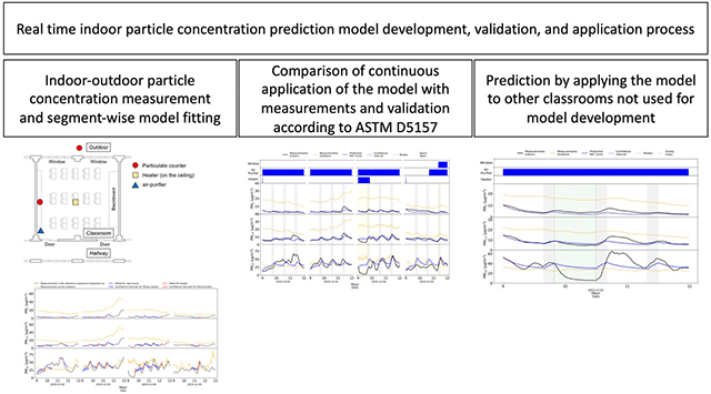
Graphical Abstract

1. Introduction

The 2021 World Health Organization report documented that in 2016, estimated premature death from exposure to particulate matter (PM) was 4.2 million people worldwide (Ambient (outdoor) air pollution 2021). This estimated annual premature death was higher than the confirmed annual deaths from the coronavirus disease 2019 (1.88 million in 2020 and 3.56 million in 2021) (Mathieu et al. 2020; COVID-19 pandemic deaths 2022). The exposure to PM is especially detrimental to young children’s health since their respiratory, immune, reproductive, central nervous, and digestive systems are not fully developed (Oliveira et al. 2019; Osseiran and Chriscaden 2017). Furthermore, because students spend most of their daytime in schools and the indoor PM levels could be higher than the outdoor levels, indoor PM exposure in classrooms may be more important than outdoor PM exposure for their health (Cooper et al. 2020; Health Risks of Indoor Exposure to Particulate Matter: Workshop Summary 2016).

Numerous studies have been published in the literature (Zhou, Yang, and Li 2021; Park et al. 2020; Othman, Latif, and Matsumi 2019; Liu et al. 2018; Mohammadyan et al. 2017; Elbayoumi et al. 2013, 2014, Elbayoumi, Ramli, and Md Yusof 2015; Yang Razali et al. 2015; Chithra and Nagendra 2014; Tran et al. 2014; Stranger, Potgieter-Vermaak, and van Grieken 2008; Weichenthal et al. 2008; Braniš, Rezácová, and Domasová 2005) that characterized indoor PM and examined factors affecting their levels in school classrooms. Table S1 in the online supplementary information (SI) file summarizes some selected articles that are most relevant to our study aims. Of those, multiple studies reported that the classroom PM levels were affected by air exchange rate, outdoor PM concentrations and size, number of students, and classroom volume. These studies also analyzed how student activity affected the generation and resuspension of coarse PM (PM_2.5–10: PM between 2.5 and 10 μm in aerodynamic diameter) and PM₁₀ (PM < 10 μm in aerodynamic diameter) (Zhou, Yang, and Li 2021; Park et al. 2020; Othman, Latif, and Matsumi 2019; Liu et al. 2018; Mohammadyan et al. 2017; Elbayoumi et al. 2013, 2014, Elbayoumi, Ramli, and Md Yusof 2015; Yang Razali et al. 2015; Chithra and Nagendra 2014; Tran et al. 2014; Stranger, Potgieter-Vermaak, and van Grieken 2008; Weichenthal et al. 2008; Braniš, Rezácová, and Domasová 2005). Chatzidiakou, Mumovic, and Summerfield (2012) found that climatic factors, traffic volume, class schedules, occupant density, and building performance affected indoor pollution levels, and that indoor plants, building materials, and indoor human activity contributed to PM generation or resuspension of settled PM on indoor surfaces. They also observed that difference in the measurement method (gravimetric versus light scattering) among the studies were one of the factors affecting the variation in PM measurements. The indoor/outdoor (I/O) ratios of PM₁₀, PM_2.5 (fine particulate, PM < 2.5 μm in aerodynamic diameter), and PM₁ (PM < 1 μm in aerodynamic diameter) concentrations during the school hours were all greater than unity. They also reported that the classroom levels of PM_2.5 and PM₁ were strongly correlated with their outdoor levels while the classroom levels of indoor PM₁₀ were weakly correlated with outdoor PM₁₀, especially when school buildings were unoccupied and there was heavy traffic volume around school buildings. Based on these observations, the authors concluded that poor performance of building envelopes was mostly responsible for the high infiltration of outdoor PM (Chatzidiakou, Mumovic, and Summerfield 2012). However, some other research teams found that the indoor concentrations of PM_2.5 were not correlated with the outdoor concentrations (Othman, Latif, and Matsumi 2019; Yang Razali et al. 2015).

All research in Table S1 analyzed the average PM concentrations over time, except for the study by Chithra and Nagendra (2014). However, the average PM levels do not properly represent variation of PM concentrations over time. To better understand indoor PM dynamics in particle penetration, removal, generation, and resuspension, the monitored real-time concentrations should be analyzed instead of the average PM levels. Through the analyses of monitoring data, researchers can develop dynamic prediction models that can forecast changes in indoor PM concentrations over time. Dynamic prediction models that describe the relationship between the inputs and outputs of a system can be classified into three types (Li et al. 2021): the white-box model, which utilizes only theoretical structure; the black-box model, which describes the relationship without any theoretical consideration; the grey-box model, which considers some theoretical structure and reflects the observed relationship using measured data. Chithra and Nagendra (2014) predicted indoor PM₁, PM_2.5, and PM₁₀ using a grey-box model in the form of differential equations considering the infiltration rate, deposition velocity, and particle generation terms. They estimated indoor generation and resuspension rate from a regression analysis using indoor and outdoor concentrations. Indoor generation and resuspension rate of the PM_2.5–10 was six times larger than that of PM_2.5. The coefficients of determination ($r^2$) for PM₁ and PM_2.5 measurements and model predictions were marginal (0.85 and 0.8, respectively) according to the ASTM D5157 standard, whereas it was low ($r^2=0.2$) for PM₁₀. Park et al. (2022) developed a grey-box model for an office room to predict dynamic change of indoor PM concentrations using information on outdoor PM concentrations, the number of occupants, and air-purifier operation. The dynamic model allowed them to quantitatively analyze the monitored PM data and to compare the PM transport mechanisms (particle penetration through infiltration, removal, and generation/resuspension) by particle size.

This study aims to create grey-box models that can predict indoor PM concentrations based on PM concentrations measured inside and outside of classrooms in elementary schools for a short period and to devise methods for effectively operating and scheduling engineering means such as portable air purifiers to reduce indoor PM level. In analyzing predicted indoor PM concentration variations using the developed prediction models, we identified the causes of significantly increased PM concentrations inside school classrooms. We will present these findings to help set future guidelines for managing indoor PM concentrations in classrooms.

2. Theory and methods

2.1. Theory

Equation (1) describes time evolution in indoor PM concentration. The terms on the right-hand side represent penetration of outdoor PM (first term), removal due to exfiltration and deposition (second term), and indoor generation (third term) (Park et al. 2022; Zhou, Yang, and Li 2021; Chithra and Nagendra 2014).

$$\frac{d{C}_{in}}{dt}=ACH\cdot P\cdot C_{out}(t)-(ACH+k)\cdot C_{in}(t)+\stackrel{.}{s}$$ (1)

where $C_{in}$ is the indoor PM concentration (μg/m³), $C_{out}$ the outdoor PM concentration (μg/m³), $ACH$ the air change rate (per hour), $P$ the penetration factor (no unit), $k$ the particle deposition rate (per hour), and s the particle generation or resuspension rate per volume per hour (μg/m³/h). If an initial value of the indoor PM concentration (i.e., $C_{in}(t=0)$) and the values of model parameters ($ACH$, $P$, $k$, and $\stackrel{.}{s}$) are provided, integrating the Equation (1) will yield the indoor PM concentration at time $t$, $C_{in}(t)$ with outdoor PM concentrations as input data. The values of the model parameters can be estimated based on the theoretical relationships as in the case of Chithra and Nagendra (2014). However, each parameter can be a complex function of the volume of the room, meteorological conditions, indoor-outdoor temperature difference, particle size distribution, number of occupants, windows/doors operating conditions that can vary by classroom and school. Equation (1) can be further simplified by combining the model constants $ACH$ · $P$ as $P^{\prime }$ and $ACH+k$ as $k^{\prime }$, to reduce the number of unknown parameters.

$$\frac{d{C}_{in}}{dt}=P^{\prime }\cdot C_{out}(t)-k^{\prime }\cdot C_{in}(t)+\stackrel{.}{s}$$ (2)

In this simplified equation, the model parameters $P^{\prime }$, $k^{\prime }$, and $\stackrel{.}{s}$ can be determined using the least squares method by minimizing the deviation between the model fitted concentrations $C_{in.model}(t)$ and the monitored indoor PM concentrations $C_{in}(t)$. In this study, these parameters were treated as functions of PM size (PM₁, PM_2.5, and PM₁₀), operation of windows and doors (open/closed), air-purifier operation (on/off), and class schedule (class time [reduced occupants’ activity] versus break time [elevated occupants’ activity]). For example, when the windows and doors are open during the breaks, ${\mathrm{P}}^{\prime }$ and ${\mathrm{k}}^{\prime }$ will increase as ACH increases. (i.e., ${\mathrm{P}}_{\text{class}}^{\prime }\le {\mathrm{P}}_{\text{break}}^{\prime }$, and ${\mathrm{k}}_{\text{class}}^{\prime }\le {\mathrm{k}}_{\text{break}}^{\prime }$) Similarly, air-purifier operation and the elevated student activity level during the break time will increase ${\mathrm{k}}^{\prime }$ and $\stackrel{.}{\mathrm{s}}$, respectively. (i.e., ${\mathrm{k}}_{\text{no}\text{AP}\text{operation}}^{\prime }\le {\mathrm{k}}_{\text{AP operation}}^{\prime }$, ${\stackrel{.}{\mathrm{s}}}_{\text{class}}\le {\stackrel{.}{\mathrm{s}}}_{\text{break}}$) Therefore, the model parameters should be determined by classroom operating condition (on windows, doors, a heater, or an air purifier), student activity, and particle size. In our study, school class schedule was categorized into class time or break time to represent student activity, adopting the approach by Zhou, Yang, and Li (2021) and then we estimated the model parameters $P^{\prime }$, $k^{\prime }$, and $\stackrel{.}{s}$ for each school with different classroom operating condition by school class schedule and particle size (PM₁, PM_1–2.5 [PM_1–2.5: PM between 1 and 2.5 μm in aerodynamic diameter], and PM_2.5–10). If we had data from an extended measurement period, it would also be possible to analyze the effects of climate, such as wind speed, wind direction, indoor-outdoor temperature difference, and others, on the model parameters. However, as shown in Table 1, indoor and outdoor PM concentrations were measured for a short period for each school classroom, so it was assumed that there was no impact due to climate changes.

Table 1.

PM monitoring time, classroom operating conditions, and the number of students for each reference classroom in four schools used in development of prediction models.

School	Year of completion	Area (m2)	Height (m)	Volume (m3)	Monitoring time		Baseline operating conditions of reference classroom	Number of students for the reference class	Airtightness for reference classroom (h−1)
					Start	End
A	1975	65.10	2.88	187.49	7 Oct 2019	11 Oct 2019	Windows closed, air purifier off	23	6.42
B	1977	65.44	2.80	183.23	11 Nov 2019	18 Nov 2019	Windows closed, air purifier off	25	15.28
C	1972	61.83	2.64	163.23	2 Dec 2019	5 Dec 2019	Windows closed, air purifier on	24	15.72
D	2007	69.22	2.64	182.47	9 Dec 2019	12 Dec 2019	Windows closed, air purifier on	21	15.86

2.2. Measurements

Indoor and outdoor PM concentrations were simultaneously monitored for multiple days in multiple classrooms (2 or 3 classrooms) in each of the four elementary schools (A–D) in Seoul, South Korea. Using these monitoring data, we analyzed the effects of the student activity levels and the outdoor PM concentrations on the indoor PM concentrations. Table 1 describes the monitoring period and classroom operating conditions for each reference classroom by school. Reference classroom is the classroom operating mainly under baseline conditions which are windows closed and air purifier on or off (depending on school) for development of a dynamic model. PM data were monitored throughout the whole measurement period in the reference classroom designated as “a” in each school. For the other two classrooms (b and c) in each school, PM data were monitored every other day due to the limited number of available instruments.

Figure 1 depicts the layout of the classroom and the indoor and outdoor monitoring locations. Indoor and outdoor PM number concentrations were monitored at the rear of the classroom and in the outdoor playground using optical particle counters with 31 particle-size channels (between 0.25 and 32 μm) (Model 11-A GRIMM Aerosol Technik, Ainring, Germany) assuming the complete mixing and homogeneous concentration condition. All indoor PM samplers and monitors were located on top of a 1.2 to 1.5-m-high shelf at the back of each classroom to minimize interference with a class activity. Outdoor sensors were located outside classrooms at 1.5 m height using tripods. In order to reflect the actual occupants’ activity environment in the measurement, it is necessary to select a measurement point that does not interfere with the activity. Generally, the center of the classroom might be the representative measurement point of the room. However, in actual living conditions experiments, the classroom center may interfere with the occupants’ activities, making it challenging to reflect general activity conditions. Therefore, the back of the classroom was selected as the measurement point. PM concentrations can vary not only temporarily but also spatially. Therefore, obtaining more information can be more helpful by using multiple sensors to measure and identify distribution. However, due to limitations in the number of sensors available and according to the measurement methods of previous researchers (Park et al. 2022; Zhou, Yang, and Li 2021; Othman, Latif, and Matsumi 2019; Liu et al. 2018; Mohammadyan et al. 2017; Elbayoumi et al. 2013, 2014, Elbayoumi, Ramli, and Md Yusof 2015; Yang Razali et al. 2015; Chithra and Nagendra 2014; Tran et al. 2014), the assumption that indoor and outdoor particulate matter concentration is well-mixed and homogeneous was adopted. The indoor and outdoor PM concentrations were collected simultaneously. Refer to Figure S1 in the (SI) for the pictures of typical sensor locations.

Figure 1.

The classroom layout and locations of particle counters, heater, and air purifier.

The year of completion of four elementary schools (A-D) were 1975, 1977, 1972, and 2007, respectively. As of the measurement date, all schools except school D were over 40 years old. Furthermore, the airtightness performance (i.e., ACH @50Pa) of each school classroom, as determined through the fan pressurization test (Blower door test system, Minneapolis DG-700, The Energy Conservatory, USA), was found to be 6.42, 15.28, 15.72, and 15.86 (1/h), respectively, which indicated building envelope of School A protected the infiltration and PM penetration much better. Figure S2 in the SI shows the logarithmic plot of the fan pressurization test result for reference classrooms in A-D schools and a representative photo of the test installation. No clear correlation was established between the airtightness performance and the year of building completion. All target classrooms were designed with one exterior-facing wall comprising windows and two sliding doors connecting to the corridor. All the windows and doors had the same area. Notably, these classrooms were not equipped with mechanical ventilation systems. The flooring of the classrooms was constructed of wood, while the walls were finished with a painted surface. The desks and chairs within the classrooms were composed of a combination of iron and wood materials. Additionally, the windows facing the exterior had been retrofitted with double-paned glazing to enhance the building envelope’s thermal insulation and airtightness performance.

Measurements of the number concentrations were recorded every minute between 8:00 AM and 3:00 PM during the school hours. Using manufacturer’s firmware, the mass concentrations were calculated from the number concentrations and then corrected with the gravimetric correction factor determined with a gravimetric particulate sampler (KMS-4100, Kemik Corporation, Seongnam, South Korea) with an airflow rate of 5 L min⁻¹. Finally, data from the 31 channels were then collapsed into PM₁, PM_2.5, and PM₁₀ to calculate cumulative mass concentrations of each size of PM.

Each and every classroom was equipped with a portable air purifier (CADR = 13 m³/min, AX100N4020WD, Bluesky, Samsung, Seoul, South Korea) and a heat pump installed with a pre-dust-filter serving as an air conditioner or a heater.

The movement of all students for the moving classes and changes in the classroom environment, such as sudden increases in activity during class and the open status of windows and doors, were recorded by observers every 10 min and are represented in Figures 2-9. As the measurements were not continuous, there may be missing events in the record; however, we believe that overall significant observations are reflected.

Figure 2.

Comparison of the predicted and measured values in reference classroom (a) of school A. The predictions were estimated for the baseline conditions (windows closed and air-purifiers not operating) in Table 1. Blue solid bars in the top three rows in the above plots denote the periods when windows were open, and the air-purifier/heater operated. The black and orange solid lines represent the indoor and outdoor measurements. The dashed blue lines are the model predictions, and the blue shaded areas are the confidence intervals of the predictions. The grey-shaded areas represent regular breaks. The green shaded areas represent the empty periods due to moving classes.

Figure 9.

Comparison of the predicted and the measured PM levels in classrooms (b) and (c) of school D. Refer to the captions of previous figures for the details of symbols.

2.3. Model development

Figure S3 in the SI presents the actual monitoring data (black and orange lines for indoor and outdoor data, respectively) and model fitted indoor PM concentrations (blue and red dashed lines for class and break times, respectively) of PM₁, PM_2.5, and PM₁₀ in the reference classroom for each of the four schools. Refer to Figure S3 in the SI for detailed explanation of fitting results.

In Table 2, it can be observed that the model constants for School A are lower than other schools in general because the airtightness of School A, as presented in Table 1, is superior to other schools. With good airtightness, there is a lower infiltration rate (ACH), leading to reduced PM penetration and, as a result, lower values for ${\mathrm{P}}^{\prime }(=\text{ACH}\cdot \mathrm{k})$ and ${\mathrm{k}}^{\prime }(=\text{ACH}+\mathrm{k})$.

Table 2.

Estimated model parameters and their uncertainties with 95% confidence levels for each class schedule (class and break time) using the actual measurements monitored under the conditions satisfying the baseline classroom operating conditions in Table 1.

School (classroom)	PM size	Class time			Break time
		$P^{\prime }$	$k^{\prime }$	$\stackrel{.}{s}$	$P^{\prime }$	$k^{\prime }$	$\stackrel{.}{s}$
A (a)	PM1	0±0.14	0.64±0.09	3.72±3.31	0.30±1.10	0.64±0.44	3.72±23.7
	PM1–2.5	0±0.26	0.77±0.25	0±2.73	1.06±0.29	0.77±0.94	11.4±6.67
	PM2.5–10	0±0.25	1.32±0.37	1.33±24.0	1.06±0.13	1.32±1.11	134±61.3
B (a)	PM1	0.87±0.44	1.79±0.79	7.51±3.65	1.02±0.19	1.98±0.37	7.51±2.81
	PM1–2.5	0.58±0.66	2.46±0.40	15.2±6.66	0.58±2.88	2.46±2.01	57.8±30.7
	PM2.5–10	0±0.90	3.63±0.50	128±34.3	0±8.48	3.63±2.52	519±206
C (a)	PM1	0.31±0.03	3.68±0.11	3.10±0.25	2.80±2.91	11.1±15.4	3.10±25.5
	PM1–2.5	3.34±0.86	2.98±0.55	1.22±2.85	3.34±1.88	2.98±0.99	10.3±8.64
	PM2.5–10	0.60±0.53	3.93±0.93	87.4±25.9	2.64±2.08	3.93±1.42	143±57.0
D (a)	PM1	0.10±0.01	2.96±0.07	18.6±1.19	0.19±0.41	2.96±4.83	77.3±53.8
	PM1–2.5	0±0.11	2.51±0.53	13.0±3.66	0.84±0.45	2.51±1.44	25.1±12.1
	PM2.5–10	0±0.49	2.42±0.89	47.0±32.4	0±0.59	2.41±1.00	204±38.4

The changes in indoor PM concentrations during the model development can be reflected on more than one parameter in Equation (2). For example, when indoor airborne PM concentration increases, it could be from the increase in outdoor PM penetration (first collective term, $P^{\prime }$) or indoor generation and/or resuspension (third collective term, $\stackrel{.}{s}$) in Equation (2). However, these underlying individual mechanisms could not be accurately allocated into the corresponding parameters because we used the simplified collective coefficients as shown in Equation (2) for the model development. This may be the reason why some parameters were estimated to be zero as shown in Table 2 although they may not be truly zero. Also, the effects of penetration and generation/resuspension of fine dust in Equation (2) all increase indoor PM concentrations. It is not easy to distinguish these using data measured under non-interfered conditions, referred to as a confounding effect. The abnormally large size of the generation/re-emission coefficients of PM₁ at School D during breaks is due to the use of fewer measurement values during break time than class time to estimate the model coefficients, resulting in a confounding effect that leads to a penetration effect being reflected as a generation/resuspension effect. However, the developed models with three parameters collectively explained well the changes in indoor PM concentrations as demonstrated in model validation and discussed in the comparison of predicted concentrations with measured ones in the following sections.

The impact of the clean air delivery rate (CADR) on the removal coefficient ${\mathrm{k}}^{\prime }$ of an air purifier has been reported by Mølgaard et al. (Mølgaard et al. 2014) as shown in Equation (3). According to this equation, the schools C and D operating air purifiers should have ${\mathrm{k}}^{\prime }$ values of at least 4.9, which they do not meet.

$$k=\frac{\text{CADR}({\mathrm{m}}^3∕\text{hour})}{\mathrm{V}({\mathrm{m}}^3)}$$ (3)

However, the determination of CADR is a value that is determined for specific pollutants such as smoke, dust, and pollen under the condition that the air purifier’s filter is in a new state and operating at maximum capacity, and does not reflect actual operating conditions of the air purifier. Furthermore, the determined model coefficient ${\mathrm{k}}^{\prime }$ also takes into account the effect of exfiltration, making it more challenging to provide a physical explanation for the determined model coefficient. However, the purpose of developing the model in this study is to predict the indoor PM concentration according to the change in outdoor PM concentration under various conditions and to determine the countermeasures, including the operation of the air purifier, using this prediction. Therefore, it is a suitable model for this purpose.

2.4. Model validation

The fitting accuracy of the developed models was evaluated according to the ASTM D5157 standard that provides guidance for statistical evaluation of the IAQ model (Conshohocken 2013). In this study, the model performance (accuracy) metrics were the correlation coefficient ($r$), slope ($b$), and intercept ($a$) of the linear regression between the observed and model-fitted values, normalized mean squared error ($NMSE$), fractional bias ($FB$), and similar index of bias based on variance ($FS$). They were calculated as shown in Equations (SI1)-(SI6) in the SI. The acceptable ranges of the model performance metrics for an adequate model were $r\ge 0.9$, $0.75\le b\le 1.25$, $\mid a\mid \le 0.25{\overline{C}}_o$, $NMSE\le 0.25$, $\mid FB\mid \le 0.25$, and $\mid FS\mid \le 0.5$ (Conshohocken 2013). Refer to the SI for further information.

Table 3 presents the calculated model performance metrics of our developed models, where ${\overline{C}}_o$ represents the mean of an observed variable. All parameters, except for those of PM₁₀ in school C, were within the acceptable ranges specified in ASTM D5157. Model fit was excellent for PM₁ and PM_2.5 in all schools while the accuracy was relatively low for PM₁₀ compared to those for PM₁ and PM_2.5. The accuracy metrics for PM₁₀ were within the acceptable ranges for schools A, B, and D but marginal for school C. It is likely that the indoor concentration in school C was strongly influenced by high generation and resuspension of indoor coarse particles from unpredictable students’ activity (Park et al. 2020; Chithra and Nagendra 2014; Braniš, Rezácová, and Domasová 2005) that happened under the non-interfered condition of the observational study. Using the developed models from the reference classroom (a) data, we predicted indoor PM concentrations in other classrooms (b and c) in each school where we compared them with the measured concentrations. We then calculated model prediction accuracy. The findings are presented in the results and discussion section below.

Table 3.

Model performance metrics^* for the reference classroom in each school.

School	size	$r$	$b$	$a∕{\overline{C}}_0$	$NMSE$	$FB$	$FS$
A	PM1	0.993	0.968	0.036	0.004	0.004	−0.052
	PM2.5	0.984	0.977	0.024	0.004	0.001	−0.015
	PM10	0.948	0.893	0.109	0.010	0.001	−0.108
B	PM1	0.986	0.969	0.035	0.004	0.004	−0.035
	PM2.5	0.983	0.995	0.008	0.002	0.003	0.024
	PM10	0.933	0.831	0.174	0.012	0.005	−0.231
C	PM1	0.980	0.948	0.053	0.014	0.002	−0.064
	PM2.5	0.923	0.809	0.186	0.019	−0.006	−0.264
	PM10	0.720	0.476	0.517	0.057	−0.007	−0.784
D	PM1	0.941	0.837	0.165	0.022	0.003	−0.233
	PM2.5	0.935	0.848	0.152	0.014	0.001	−0.194
	PM10	0.900	0.797	0.204	0.012	0.001	−0.243

^*The acceptable ranges of the model performance metrics for an adequate model were $r\ge 0.9$, $0.75\le b\le 1.25$, $\mid a\mid \le 0.25{\overline{C}}_o$, $NMSE\le 0.25$, $\mid FB\mid \le 0.25$, and $\mid FS\mid \le 0.5$.

3. Results and discussion

As described in the previous section, the initial PM concentration, ${\mathrm{C}}_{\text{in}}(t=0)$, is required to predict the indoor PM concentration at time $t$, ${\mathrm{C}}_{\text{in}}(\mathrm{t})$. To predict PM concentrations for the first class, the very first measurement of the first-class time was used as the initial concentration. The initial concentration could also be obtained by either solving the equation assuming steady state by setting $\frac{{\text{dC}}_{\text{in}}}{\text{dt}}=0$ and $\stackrel{.}{\mathrm{s}}=0$ in Equation (2) using the average outdoor PM concentration between after school on the day and before the first class on the next day, or integrating Equation (2) with the outdoor PM histories. Also, we are currently working on estimating the initial concentration for the model prediction, using forecasted outdoor PM concentrations (World Air Quality Index project 2022) under the condition of no monitoring data. For the initial concentration for the break time prediction, the last predicted value during the previous class time was used. For the subsequent class time prediction, the last predicted value during the previous break time was also used as the initial concentration. Indoor PM concentrations were then predicted by integrating model Equation (2) with those initial concentrations and the estimated model parameters (Table 2). Figures 2 through 9 compare the predicted indoor PM concentrations with the measured concentrations by school and classroom. These figures showed that the measured indoor PM₁ and PM_2.5 concentrations were consistently lower than the outdoor concentrations, except for 14 November and 5 December. On these two days, the indoor concentrations were comparable with outdoor concentrations, likely due to low outdoor PM concentrations. Conversely, indoor PM₁₀ concentrations containing coarse PM were generally higher than outdoor concentrations. These results were consistent with previous findings that outdoor PM_2.5 was the primary source of indoor PM_2.5 (penetration) while indoor occupants or PM settled on indoor surfaces were the main sources of indoor coarse PM (generation and resuspension by occupants’ indoor activities) (Park et al. 2020; Yang Razali et al. 2015; Tran et al. 2014; Braniš, Rezácová, and Domasová 2005). The prediction model was developed for a reference classroom in each of the four schools to reflect differences in school location, building orientation, climate conditions, performance of building envelopes, and operating conditions among schools.

3.1. Analysis of data from school A

Figure 2 compares the predicted indoor PM concentrations under the assumption of the baseline classroom (a) operating conditions in Table 1 (windows closed and air purifier not operating) with the monitored indoor and outdoor PM concentrations in the reference classroom (a) of school A. However, during the measurement period except for the times under the baseline operating conditions, the windows were mostly open. Therefore, the measured indoor PM concentrations were higher than the values predicted under the assumptions of windows closed. When windows are open, $P^{\prime }$ and $k^{\prime }$ increase with the air change rate in Equation (2) (Liu et al. 2018). However, because the effect of the increase in $P^{\prime }$ would exceed that in $k^{\prime }$ (under the condition of air purifier not operating), the indoor PM concentrations would be dominantly affected by $P^{\prime }$. This interpretation seemed to be justified by the observations that when the classroom windows were closed at 9:45 AM on 10 October and at 10:30 AM for approximately 1 h, on 11 October, the measured PM₁ and PM_2.5 concentrations were significantly decreased. As the windows were open again after the period on 11 October, the measured indoor PM concentrations approached the outdoor concentrations.

During the measurements, only the status of windows and doors being open or closed was recorded, and the degree of their openness was not monitored. When the windows and doors are fully open, the ventilation rate increases and the indoor PM concentration will quickly approach the outdoor PM concentration. In contrast, if they are only partially open, it will take longer for the indoor PM concentration to reach the outdoor PM concentration. This explains why there is a difference between the indoor and outdoor PM concentrations in Figure 2, even though the windows are open.

Figure 3 compares the predicted indoor PM concentrations with the measured concentration in non-reference classrooms (b) and (c). The predicted indoor PM₁ and PM_2.5 concentrations of classroom (b) with the air purifier operating and windows closed were higher than the measured concentrations. Thus, the difference between the model predictions and actual measurements in classroom (b) represents the amount of PM removed by the air purifier. Between 10:40 and 10:50 AM, all students moved out to other classrooms, and the movement activity of a group of students resulted in substantial increase in the concentration of PM_2.5–10 as seen as a large peak of indoor PM₁₀ concentrations in Figure 3. Indoor PM_2.5 and PM₁₀ concentrations rapidly dropped from 10:50 AM until 11:30 AM on 7 October when no students were in the classroom (i.e., zero generation and resuspension: $\stackrel{.}{s}=0$ in the Equation (2) under the assumption of no other indoor PM generation source). The mean predicted indoor concentrations of PM₁ and PM_2.5 (under the assumption of no air purifier operation and no windows open) in the classroom (b) on 7 October were 5.64 and 9.43 μg/m³, respectively (Figure 3). With an operating air purifier, the mean measured concentrations were 2.60 μg/m³ for PM₁ and 7.05 μg/m³ for PM_2.5, indicating that predicted removal efficiency of the air-purifier was approximately 54% for PM₁ and 25% for PM_2.5. However, the mean value of the predicted indoor PM₁₀ concentration (32.2 μg/m³) on 7 October was lower than the measured concentration (45.9 μg/m³), and the difference was likely to be explained by low removal efficiency of air-purifier for the large PM (Park et al. 2022) and the increase in PM_2.5–10 generation and resuspension by increased students’ activity during the break times (Zhou, Yang, and Li 2021; Yang Razali et al. 2015).

Figure 3.

Comparison of the predicted and measured values in classrooms (b) and (c) of school A. Refer to the caption of Figure 2 for the details of the symbols.

On 10 October, the operating conditions for the classroom (c) between 9:00 and 10:40 AM were the same as those for the reference classroom (a) that were used for the model development (Table 1). During this time, all predicted PM concentrations well agreed with the actual measurements, which demonstrated accuracy of the developed prediction model. All students had moved out of the classroom during 9:50–10:30 AM followed by a rapid increase in measured PM₁, PM_2.5, and PM₁₀ concentrations when they returned to the classroom (Ferro, Kopperud, and Hildemann 2004; Thatcher and Layton 1995). The increased PM concentrations then decreased rapidly with the operation of the air purifier in the classroom (c) (Figure 3). The concentrations of PMs in classroom (c) on 10 October, as shown in Figure 3, exhibited a peak after the designated break time from 10:30 to 10:50 AM when many students returned to the classroom after a moving class. While the depicted break times in the figure aligned with the school’s academic operating guidelines, students’ actual entrance time into the classroom was later than the designated time.

Comparison of the predictions with the measurements in the two non-reference classrooms in school A indicated that operating the air purifier decreased the indoor PM₁ and PM_2.5 concentrations significantly (Figure 3). Table 2 also indicated that the $k^{\prime }$ values for classrooms with air purifier turned off in school A was much smaller than those of schools C and D ($k_A^{\prime }\ll k_C^{\prime },k_D^{\prime }$) owing to lower $ACH$ in Equation (1) due to better airtightness of School A and augmented $k$ in Schools C and D with an air purifier operating during the class time. In addition, the indoor PM₁ and PM_2.5 concentrations tended to follow outdoor PM levels when the windows were open. These findings indicated that classroom operating conditions greatly influenced indoor PM concentrations. And our prediction model would inform school management of when an air purifier needs to be operated to minimize occupants’ exposure to PM instead of leaving it turned on all day, which would help the management optimize the operating costs by decreasing the use of filter materials and electricity.

If the allowable limit of PM_2.5 and PM₁₀ concentrations in the classroom are set at 35 and 75 μg/m³, respectively, and the decision on whether to operate an air purifier was made based on the model’s predicted values, it would likely be that the air purifier would not be operated in classrooms (b) and (c) as the predicted concentrations are consistently below the given limits. However, it has been observed that during events when all students are entering and exiting the classroom simultaneously, the indoor PM concentrations could increase significantly beyond the values predicted by the model. Therefore, the model can be improved to consider such events, or guidelines can be provided to ensure that the air purifier is operated during these events.

3.2. Analysis of data from school B

Figure 4 compares the predicted indoor PM concentrations under the baseline operating conditions of the reference classroom in Table 1 with the monitored indoor and outdoor PM concentrations in classroom (a) of school B. When the classroom operating conditions were the same as baseline conditions on 11 and 13 November, the predicted concentrations generally agreed well with the actual measurements. However, starting at 10:50 AM on 13 November, the student’s activity level increased and thus the concentrations of PM_2.5 and PM₁₀ also rapidly increased. While the classroom heater was operating on 12 and 18 November, the predicted levels of indoor PM were higher than the actual measurements, indicating removal of indoor PM by the pre-filter installed in the heater. The removal efficiencies for PM were estimated based on the difference between the predicted and measured values using the data between 9:00 and 10:30 AM on 12 November. The removal efficiencies for PM₁, PM_2.5, and PM₁₀ on the day were 26, 28, and 19%, respectively, while they were 32%, 50%, and 40%, respectively, when the data between 9:00 and 10:30 AM on 18 November were used. The pre-filter used in air conditioning systems is typically designed to remove coarse particles, and it is unusual that the PM₁ removal efficiency was as high as 26% and 32%, respectively. However, the reasons for such high efficiencies are not clear and require further explanation.

Figure 4.

Comparison of the predicted and measured values in classroom (a) of school B. The red and yellow shaded areas show active class hours and class hours with doors open. Refer to the caption of Figure 2 for details of other symbols.

In classroom (b) of school B, the predicted values under the reference classroom operating conditions (windows closed and air purifier off) were similar to the actual measurements under the conditions of windows open and air purifier operating (Figure 5). Under these actual conditions, it is likely that the reduction of indoor PM by an air-purifier was offset by penetration of outdoor PM through windows opened. In classroom (c), the predicted levels were generally higher than the actual measurements that were decreased by filtration effect of the operating air purifier. The removal efficiencies of air purifier estimated based on the differences between the measured and predicted values between 9:00 AM and 11:30 AM on 12 November in Figure 5 were 31%, 41%, and 29% for PM₁, PM_2.5, and PM₁₀, respectively. The PM removal efficiencies of the heater were as high as those of the air purifier in school B.

Figure 5.

Comparison of the predicted and measured values in classrooms (b) and (c) of school B. Refer to the caption of Figure 4 for the details of legends..

In the previous study (Park et al. 2022), we reported, based on the measurement results for an office in a college, that the effectiveness was greater than 75% for PM smaller than 1 μm in diameter and significantly decreased as particle size approached the 1–3 μm range. Then, it substantially increased for particles approximately 3–4 μm in size. For PM larger than 4 μm, again, the effectiveness sharply declined. The particle removal effectiveness of the air purifier for PM_2.5 and PM₁₀ was estimated to be 86.4% and 86%, respectively. The large deviations in the effectiveness between the studies could be attributed to differences in the test conditions, such as cleaning space volume (45 m² for the previous study and 65 m² for the current study) and air purifier maintenance status.

3.3. Analysis of data from school C

The PM concentrations in the classrooms in school C were measured in the cold winter. During the monitoring, the air purifier was operating most of the time with windows closed, which is equivalent to the reference operating condition for the classroom (a) in the school C (Table 1). In general, the measured indoor PM concentrations were lower than those in schools A and B. Figure 6 compares the model predictions with the actual measurements in the classroom (a). Because of a higher removal coefficient of the air purifier during the class time than that of the classroom (a) in school A ($(k_C^{\prime }>k_A^{\prime })$) in Table 2), the indoor PM concentrations during the class time decreased more rapidly compared to the classroom (a) in school A. Similar to the report of a study in India (Chithra and Nagendra 2014), our model predictions for PM₁ and PM_2.5 were more accurate than PM₁₀ that includes coarse particulates strongly affected by students’ activity.

Figure 6.

Comparison of the predicted and the measured concentrations in classroom (a) of school C. The predictions were estimated for the baseline conditions (windows closed and air purifier operating) in Table 2. Refer to the captions of previous figures for the details of symbols.

The predicted concentrations of PM_2.5 and PM₁₀ in the first period (9:00–9:40 AM) of classroom (a) on 4 December (Figure 6) were higher than the actual measurements when the air purifier or the heater were operating. Operating both an air purifier and a heater (the first period on 4 December) helped further remove PM than operating an air purifier alone. The predicted and measured concentrations for PM₁ and PM_2.5 became similar after the heater was turned off because the classroom operating conditions became the same as the baseline operating conditions for the model development. The air purifier did not operate until 10:30 AM on 5 December and the measured indoor PM₁ and PM_2.5 concentrations were higher than the model predictions under the reference conditions (windows closed and air purifier operating). The mean predicted values were 2.31 μg m³ for PM₁ and 5.76 μg m³ for PM_2.5 while the mean measured indoor PM₁ and PM_2.5 concentrations were 5.41 and 7.57 μg/m³, respectively, under the condition with an air purifier not operating. These results indicated that 57.3% of PM₁ and 23.9% of PM_2.5 could have been removed by operating the air purifier.

Generally, PM concentrations decreased during the class time and increased during the break time. However, during the first period (9:00–9:40 AM) in classroom (a), both predicted and measured indoor PM₁₀ concentrations at the start were low and increased as the class continued while in classroom (b), the initial PM₁₀ concentration were high and decreased as the class continued. These results could be explained by a mechanism of transition to the steady-state condition. The steady-state indoor PM₁₀ concentration is shown in Equation (4), which was derived by setting the left-hand side of Equation (2) to zero, i.e., ($\frac{d{C}_{in}}{dt}=0$).

$$C_{in.steadystate}=\frac{P^{\prime }\cdot C_{out}(t)+\stackrel{.}{s}}{k^{\prime }}$$ (4)

Indoor PM₁₀ concentrations in classroom during the night with no activity can decrease due to gravitational sedimentation, which is the effect of $k^{\prime }$ when $\stackrel{.}{s}=0$ in Equation (2). When students enter the classroom as school starts, $C_{in.steadystate}$ also increases with generation and resuspension of PM ($\stackrel{.}{s}>0$) toward a new steady state. When the indoor PM₁₀ concentration is lower than the steady state value at a given time, indoor PM₁₀ concentrations tend to increase toward a new and higher steady state value that was created by the students’ entry to the classroom, which was the case for the classroom (a). The initial concentration of PM₁₀ in the classroom (a) before the start of the first class on 2 December 2019 read to be 19 μg/m³. When we used the model coefficients for the class time in school C (Table 2) and the average $C_{out}$ values during the first class, the new $C_{in.steadystate}$ value was estimated to be 27 μg/m³ that was increased from the initial steady state value (19 μg/m³). Therefore, the predicted PM₁₀ concentration approached the new steady state value at the end of the first class on 2 December. However, initial indoor PM₁₀ concentration in classroom (b) at the beginning of the first period was higher than the steady-state value (27 μg/m³), likely due to no AP operation before the class and high students’ activity. Therefore, the PM₁₀ concentration started to decrease toward the lower steady-state value over time as shown in Figure 7.

Figure 7.

Comparison of the predicted and measured PM concentrations in classroom (b) of school C. Refer to the caption of Figure 7 for the details of legends.

The operating conditions for the classroom (b) on 2 December (Figure 7) were the same as those for the reference classroom (a), i.e., windows closed and an air purifier operating. The pattern of changes in the PM₁ and PM_2.5 concentrations was similar between two classrooms, except that the initial PM concentrations at the beginning of the class were higher in the classroom (b) than those in the classroom (a). Figure 7 compares the model predictions performed with the high initial concentration in classroom (b) with the measured PM concentrations. Between 9:50 and 10:30 AM when the classroom (b) was empty after the students moved out, the predicted indoor PM₁₀ concentrations were much higher than the measured concentrations because there was no indoor generation or resuspension in the empty classroom. However, the effects of PM_2.5–10 generation and resuspension were apparent at 10:30 when students started to return to the homeroom classroom. The PM₁ and PM_2.5 concentrations did not increase as much as PM₁₀ with students’ activity because of the operating air purifier that more effectively removed PM₁ and PM_2.5 than PM₁₀. The predicted PM concentrations during the third period (10:40–11:20 AM) were lower than the measured levels because of the elevated PM levels associated with students’ return to the classroom between 10:30 and 10:40 AM.

3.4. Analysis of data from school D

Similar to school C, the PM concentrations in the classrooms in school D were measured in the cold winter when the air purifier was operating most of the time with windows closed, which is the same as the reference classroom (a) condition in the school (Table 1). Figure 8 depicts the predicted and measured values in the reference classroom (a). All classes in the school D began at 10:00 AM on 9 December. The predicted and measured PM concentrations on 9 December were similar most of the time. The measured indoor PM₁₀ concentrations were continuously reduced during the second period (9:50–10:30 AM) on 10 December in the empty homeroom classroom after all students had moved out to another classroom. The measured PM concentrations increased during C the first (09:00–09:40 AM) and fourth classes (11:30–12:10 PM) on 11 December because student activity might have been high (or the windows might have been open although it was not recorded) during the first class and hallway windows were open during the fourth class (air in hallway was affected by outdoor air more than classroom). Outdoor PM concentrations were much lower on 12 December than other days. The measured indoor PM₁ and PM_2.5 concentrations were similar to or slightly higher than the outdoor concentrations because the effects of generation and resuspension on indoor PM were likely higher than that of PM penetration from outdoors when the outdoor PM concentrations were low. Although the effect of student activity on fine PM is usually weaker than coarse PM, the effect is still not negligible if the outdoor concentration is low. Classroom PM₁₀ concentrations were less affected by the outdoor concentrations than PM₁ and PM_2.5 under the conditions with windows closed and the air purifier operating because they are mainly affected by student activity as discussed earlier. Conversely, penetration of outdoor PM was the main contributor to indoor PM₁ and PM_2.5 concentrations (Park et al. 2020; Chithra and Nagendra 2014; Braniš, Rezácová, and Domasová 2005).

Figure 8.

Comparison of the predicted and the measured PM levels in the reference classroom (a) of school D. Refer to the captions of previous figures for the details of symbols.

During the measurements in school D, the outdoor PM concentrations were high on 11 December but low on 12 December (Figure 8). The impact of outdoor PM on indoor PM through penetration depends on the outdoor PM concentration. Assuming steady state condition, rearranging Equation (4) yields Equation (5):

$$\frac{C_{in}}{C_{out}}=\frac{P^{\prime }}{k^{\prime }}+\frac{\stackrel{.}{s}}{k^{\prime }\cdot C_{out}}$$ (5)

where the first term on the right-hand side is the penetration, and the second term is the effect of indoor generation and resuspension. The fraction of penetration effect in the changes in total indoor PM concentrations can be expressed as $\frac{P^{\prime }}{k^{\prime }}∕\left(\frac{P^{\prime }}{k^{\prime }}+\frac{\stackrel{.}{s}}{k^{\prime }\cdot C_{out}}\right)$, which explains why the impact of infiltration decreases with the decrease in outdoor concentrations or becomes negligible as reported in Yang Razali et al. (2015).

Figure 9 compares the model predictions with the measurements for classrooms (b) and (c). The predicted PM₁₀ concentrations were higher than the measured ones in classroom (b) during 10:00–10:30 AM when there were no students in the classroom ($\stackrel{.}{s}=0$). Then all sizes of PM rapidly increased when students returned to the classroom of which the impact was more evident for PM₁₀ than other PM sizes although the effect was not as substantial as seen in the case of the reference classroom (a) of school A because of the operating air purifier.

In classroom (c), the heater and the air purifier were simultaneously operating for the first two periods of classes on 10 December. The actual PM₁₀ measurements lower than the predicted levels (under the classroom conditions with windows closed and only air purifier operating) were likely from the additional filtering effect of the heater. However, this combined effect was not as strong as seen in school C. Indoor PM₁₀ measurements substantially increased during the third-class period (10:40–11:20 AM) due to increased student class activity. However, the increase in the concentrations of PM₁ and PM_2.5 due to this activity was less evident as discussed earlier (Park et al. 2020; Yang Razali et al. 2015; Tran et al. 2014; Braniš, Rezácová, and Domasová 2005).

3.5. Implications for class management guidelines and limitations

In the previous sections, we discussed the predicted and measured PM levels for each classroom in four schools under different operating conditions with windows, a heater and an air purifier. The findings from the study suggested that it may be possible to develop prediction models that can guide operations of air purifiers, especially during episodes of high outdoor PM concentrations during the yellow sand dust season when sand dusts originated from the desserts in Northern China and Mongolia are transported to Korean peninsula through the industrialized areas in China (Oh et al. 2020; Lee et al. 2019). The events occur mostly in spring, and no yellow sand dust event was observed during the measurements in this study. Given the next day outdoor PM concentrations forecast using either hourly outdoor PM levels forecasted by the Korea Environment Corporation (Korea Weather Corporation 2023), or hourly air quality and pollution forecast by the World Air Quality Index project (World Air Quality Index project 2022), we can develop prediction models customized to individual schools or a group of schools and then use the developed models to predict indoor PM concentrations. Figure 10 compares the predicted indoor PM_2.5 and PM₁₀ levels in reference classrooms (windows closed and air purifier not operating) in schools A and B using the same outdoor PM measurement data collected on 11 October (measured from school A) and 13 November 2019 (from school B). Schools manage the allowable limits of PM concentration within school classrooms according to the education department’s high-concentration PM response manual. (Seoul Metropolitan Office of Education 2019) According to this manual, the current level of fine dust within classrooms is only regulated for PM_2.5 and PM₁₀. Therefore, the guidelines for the operation of air purifiers, such as those provided in Figure 10, focus solely on PM_2.5 and PM₁₀ and omit PM₁. The comparison of the predicted PM levels between classrooms helps us understand how we can modify the classroom operating condition to lower the classroom PM levels. The black solid lines in Figures 10a and b represent the control limits of PM_2.5 (35 μg/m³) and PM₁₀ (75 μg/m³) recommended by the air pollution response manual of the Seoul Metropolitan Office of Education (Seoul Metropolitan Office of Education 2019). School A could maintain indoor PM_2.5 concentrations below the control limit without operating an air purifier because the predicted levels under the reference classroom conditions were always lower than the limit. However, the predicted PM₁₀ concentrations exceeded the control limit from 09:00 to 09:15 AM and 10:40 to 11:20 AM on 11 October 2019 in Figure 10a. Thus, during the periods, the air purifier should have operated to decrease the actual PM₁₀ levels. Under the assumption that the amount of electricity needed for an air purifier to operate is proportional to the length of time it is in use, regulating the use of air purifiers by predicting indoor levels of fine dust would result in a 74% reduction in electricity usage for air purifiers in school A.

Figure 10.

Comparison of the model-predicted PM2.5 and PM10 levels (blue- and red-dashed lines for schools A and B, respectively) with the control limits (black solid lines) recommended by the air pollution response manual prepared by the Seoul Metropolitan Office of Education (Seoul Metropolitan Office of Education 2019). The orange solid lines represent outdoor PM concentrations. Figures (a) and (b) represent the predictions for a day in October (outdoor PM data from school A) and another day in November (outdoor PM data from school B), respectively.

In school B, the predicted levels of PM_2.5 under the same reference condition as classroom (a) of school A exceeded the control limit from 10:40 AM to 12:00 PM and the predicted PM₁₀ exceeded the limit most of the day. During these periods, the classroom in the school should have operated the air purifier to reduce indoor PM levels, resulting in no possible energy savings. This approach could help provide guidelines for an operation schedule of the air-purifier in each classroom. The predicted indoor concentrations of PM_2.5 and PM₁₀ in the reference classroom at school B on 13 November 2019, mostly exceeded the limit so that no energy savings were possible, whereas those at school A were mainly lower than the limit as shown in Figure 10b allowing a provisional 95% energy savings in running air purifiers. The second example in Figure 10b again confirmed that given outdoor PM concentrations the model predictions in each classroom could provide a guidance on when they should operate an air purifier to lower the indoor PM levels. Considering the number of classrooms >240,000 in South Korea (Statistics Korea 2023), the savings in each class could sum up to a significant amount. In these two examples in Figure 10, PM concentrations in the classroom of school A with windows closed and no air purifier operating were always lower than those in school B with the same classroom operating condition under the same profile of outdoor PM concentrations. This indicates that the building envelope of school A has better performed than that of school B in preventing penetration of outdoor PM into the classroom, which is supported by the better airtightness in Table 1. Therefore, such analysis using the prediction models may also provide information on prioritizing the remediation of air tightness of the school building envelopes.

The results obtained from previous model development and analysis provide implications for the guidelines on school indoor response during high-density PM events, which can be summarized as follows:

1. A predictive model, developed based on the criteria of non-operation of the air purifier and closed windows, can predict the indoor PM concentration the next day with the next day’s forecast of the outdoor PM concentration as the input. The model can be utilized as a guideline for the air purifier operation when the predicted value exceeds the limit value.

2. Within the same region, different schools or classrooms may have differences in the need for air purifier operation during high-density PM events due to differences in building envelope performance.

3. The simultaneous movement of a large number of students, such as a mobile class, can cause a sharp increase in coarse PM due to generation and resuspension, so the air purifier should be operated before and after the event.

4. The operation of devices with pre-filters, such as heaters or air conditioners, can help remove indoor PM, especially coarse PM.

5. Usually, there is a 10-min break after the class, but there may be cases where there is a 20-min break after the second class, depending on the school. During the break, PM generation and resuspension occur, leading to a sharp increase in indoor PM concentration. It is recommended to avoid extended breaks during high-density PM events.

One limitation of our study is that the prediction models were developed using measurements from a short period of time, and thus seasonal variation was not reflected in the monitored outdoor PM levels and model parameters (e.g., the change of infiltration rate with the indoor-outdoor temperature difference). A more accurate evaluation of performance of classroom operating conditions and comparisons among classrooms could be accomplished by developing models using long-term measurement data.

Another limitation is that predictions using the developed model may be only applicable to the conditions tested and for the range of measured outdoor PM levels (Figure S4) that were used for the model development in our study. In addition, because the student activity within classrooms was unpredictable or uncontrollable, it could not be considered in the model development. In our study, this resulted in some deviation of the predicted values from the measured ones during the time with high students’ activities. Forecasted PM concentrations (Hourly Air Quality and Pollution Forecast - PM2.5 and Ozone 2021) provided by government are for the larger area rather than for the specific school locations, and thus they cannot reflect the local variations of PM concentrations near schools, which may result in less accurate predictions. Studies to examine the relationships between the forecasted PM and the measured local PM concentrations would be beneficial to further refine the developed prediction models.

4. Conclusions

Our study demonstrated how to develop dynamic prediction models for classroom PM concentrations, explain potential PM transport mechanisms (infiltration, deposition, and generation), and apply them to dynamically predict indoor PM concentrations for avoidance of high indoor PM exposures. The indoor PM concentrations increased during the break between classes because of PM generation and resuspension from increased students’ activities. The group movement of students to another classroom rapidly and substantially raised indoor PM concentrations. Operation of a heater in addition to an air purifier appeared to further lower the indoor PM concentrations in the classrooms because of the additional filtration effect. It may be beneficial to conduct studies to further evaluate the combined filtration effects of the air purifier and the heater during the heating season.

As demonstrated, the indoor PM concentrations can vary widely, depending on the classroom operating conditions. Thus, the dynamic prediction models would be also valuable in developing guidelines on operating an air purifier, especially during episodes of high outdoor PM concentrations. If model predictions using forecasted outdoor PM level data (possibly provided through the school district from government forecast data) under the assumption of closed windows and no air purifier in operation exceed the control limits, an air purifier should be operated to reduce occupants’ exposures. The proper guidelines on operation of an air purifier to reduce classroom PM levels would be also helpful to reduce the operation cost of air purifiers because the dynamic prediction models could indicate specific times when they need to be operated, instead of operating all day long.

It is possible to improve or make the model under consideration more general by adding more variables. For example, by analyzing data collected over a longer period, it may be possible to include model coefficients that change based on factors such as indoor and outdoor temperature and humidity to explain variations in the transfer of fine dust due to seasonal changes. Additionally, by quantitatively measuring the degree of windows and doors opening, it may be possible to adjust model coefficients to explain variations in PM transfer, leading to a more generalized model.

References

- Ambient (outdoor) air pollution. 2021. World Health Organization (WHO). Accessed January 29, 2021. https://www.who.int/news-room/fact-sheets/detail/ambient-(outdoor)-air-quality-and-health.
- Braniš M, Rezácová P, and Domasová M. 2005. The effect of outdoor air and indoor human activity on mass concentrations of PM10, PM2.5, and PM1 in a classroom. Environ. Res 99 (2):143–9. doi: 10.1016/J.ENVRES.2004.12.001. [DOI] [PubMed] [Google Scholar]
- Chatzidiakou L, Mumovic D, and Summerfield AJ. 2012. What do we know about indoor air quality in school classrooms? A critical review of the literature. Intel. Build. Intern 4 (4):228–59. doi: 10.1080/17508975.2012.725530. [DOI] [Google Scholar]
- Chithra VS, and Nagendra SMS. 2014. Characterizing and predicting coarse and fine particulates in classrooms located close to an urban roadway. J. Air Waste Manag. Assoc 64 (8):945–56. doi: 10.1080/10962247.2014.894483. [DOI] [PubMed] [Google Scholar]
- Conshohocken W. 2013. Standard guide for statistical evaluation of indoor air quality Models 1. 97(Reapproved 2008): 3–6. [Google Scholar]
- Cooper N, Green D, Guo Y, and Vardoulakis S. 2020. School children’s exposure to indoor fine particulate matter. Environ. Res. Lett 15 (11):115003. doi: 10.1088/1748-9326/abbafe. [DOI] [Google Scholar]
- COVID-19 pandemic deaths. 2022. Accessed January 30, 2022. https://en.wikipedia.org/wiki/Template:COVID-19_pandemic_data.
- Elbayoumi M, Ramli NA, and Md Yusof NFF. 2015. Spatial and temporal variations in particulate matter concentrations in twelve schools environment in urban and overpopulated camps landscape. Build Environ. 90:157–67. doi: 10.1016/j.buildenv.2015.03.036. [DOI] [Google Scholar]
- Elbayoumi M, Ramli NA, Md Yusof NFF, and Al Madhoun W. 2013. Spatial and seasonal variation of particulate matter (PM10 and PM2.5) in Middle Eastern classrooms. Atmos. Environ 80:389–97.doi: 10.1016/j.atmosenv.2013.07.067. [DOI] [Google Scholar]
- Elbayoumi M, Ramli NA, Md Yusof NFF, Yahaya AB, Al Madhoun W, and Ul-Saufie AZ. 2014. Multivariate methods for indoor PM10 and PM2.5 modelling in naturally ventilated schools buildings. Atmos. Environ 94:11–21. doi: 10.1016/j.atmosenv.2014.05.007. [DOI] [Google Scholar]
- Ferro AR, Kopperud RJ, and Hildemann LM. 2004. Source strengths for indoor human activities that resuspend particulate matter. Environ. Sci. Technol 38 (6):1759–64. doi: 10.1021/ES0263893/SUPPL_FILE/ES0263893SI20030924_074503.PDF. [DOI] [PubMed] [Google Scholar]
- Health Risks of Indoor Exposure to Particulate Matter: Workshop Summary. 2016. Health risks of indoor exposure to particulate matter. doi: 10.17226/23531. [DOI] [PubMed] [Google Scholar]
- Hourly Air Quality and Pollution Forecast - PM2.5 and Ozone. 2021. Accessed May 5, 2021b. https://aqicn.org/forecast/.
- Korea Weather Corporation. 2023. AirKorea. Accessed January 31, 2023. https://www.airkorea.or.kr/web/.
- Lee HJ, Jo HY, Kim SW, Park MS, and Kim CH. 2019. Impacts of atmospheric vertical structures on transboundary aerosol transport from China to South Korea. Sci. Rep 2019 9:1 9 (1):1–9. doi: 10.1038/s41598-019-49691-z. [DOI] [PMC free article] [PubMed] [Google Scholar]
- Li Y, O’Neill Z, Zhang L, Chen J, Im P, and DeGraw J. 2021. Grey-box modeling and application for building energy simulation:A critical review. Renewable Sustainable Energy Rev. 146:111174. doi: 10.1016/j.rser.2021.111174. [DOI] [Google Scholar]
- Liu C, Yang J, Ji S, Lu Y, Wu P, and Chen C. 2018. Influence of natural ventilation rate on indoor PM2.5 deposition. Build Environ. 144:357–64. doi: 10.1016/j.buildenv.2018.08.039. [DOI] [Google Scholar]
- Mathieu E, Ritchie H, Rodés-Guirao L, Appel C, Giattino C, Hasell J, Macdonald B, Dattani S, Beltekian D, Ortiz-Ospina E, et al. 2020. Coronavirus pandemic (COVID-19). Our World in Data. [Google Scholar]
- Mohammadyan M, Alizadeh-Larimi A, Etemadinejad S, Latif MT, Heibati B, Yetilmezsoy K, Abdul-Wahab SA, and Dadvand P. 2017. Particulate air pollution at schools: Indoor-outdoor relationship and determinants of indoor concentrations. Aerosol Air Qual. Res 17 (3): 857–64. doi: 10.4209/aaqr.2016.03.0128. [DOI] [Google Scholar]
- Mølgaard B, Koivisto AJ, Hussein T, and Hämeri K. 2014. A new clean air delivery rate test applied to five portable indoor air cleaners. Aerosol Sci. Technol 48 (4): 409–17. doi: 10.1080/02786826.2014.883063. [DOI] [Google Scholar]
- Oh HR, Ho CH, Koo YS, Baek KG, Yun HY, Hur SK, Choi DR, Jhun JG, and Shim JS. 2020. Impact of Chinese air pollutants on a record-breaking PMs episode in the Republic of Korea for 11–15 January Atmos Environ 223:117262. doi: 10.1016/j.atmosenv.2020.117262. [DOI] [Google Scholar]
- Oliveira M, Slezakova K, Delerue-Matos C, Pereira MC, and Morais S. 2019. Children environmental exposure to particulate matter and polycyclic aromatic hydrocarbons and biomonitoring in school environments: A review on indoor and outdoor exposure levels, major sources and health impacts. Environ. Int 124:180–204. doi: 10.1016/J.ENVINT.2018.12.052. [DOI] [PubMed] [Google Scholar]
- Osseiran N, and Chriscaden K. 2017. The cost of a polluted environment: 1.7 million child deaths a year, says WHO. Accessed January 29, 2021. https://www.who.int/news/item/06-03-2017-the-cost-of-a-polluted-environment-1-7-million-child-deaths-a-year-says-who.. [Google Scholar]
- Othman M, Latif MT, and Matsumi Y. 2019. The exposure of children to PM2.5 and dust in indoor and outdoor school classrooms in Kuala Lumpur City Centre. Ecotoxicol. Environ. Saf 170:739–49. doi: 10.1016/J.ECOENV.2018.12.042. [DOI] [PubMed] [Google Scholar]
- Park JH, Lee TJ, Park MJ, Oh HN, and Jo YM. 2020. Effects of air cleaners and school characteristics on classroom concentrations of particulate matter in 34 elementary schools in Korea. Build Environ. 167:106437. doi: 10.1016/j.buildenv.2019.106437. [DOI] [PMC free article] [PubMed] [Google Scholar]
- Park SB, Park J-H, Jo YM, Song D, Heo S, Lee TJ, Park S, and Koo J. 2022. Development and validation of a dynamic mass-balance prediction model for indoor particle concentrations in an office room. Build Environ. 207:108465. doi: 10.1016/j.buildenv.2021.108465. [DOI] [PMC free article] [PubMed] [Google Scholar]
- Seoul Metropolitan Office of Education. 2019. Practical manual for dealing with high concentration of fine dust. http://buseo.sen.go.kr/view/jsp/bbsDownload.jsp?bbsCd=94&bbsSeq=7328&orderNo=1. [Google Scholar]
- Statistics Korea. 2023. KOSIS Korean statistical information service. Accessed January 18, 2023. https://kosis.kr/index/index.do.
- Stranger M, Potgieter-Vermaak SS, and van Grieken R. 2008. Characterization of indoor air quality in primary schools in Antwerp, Belgium. Indoor Air. 18 (6):454–63. doi: 10.1111/J.1600-0668.2008.00545.X. [DOI] [PubMed] [Google Scholar]
- Thatcher TL, and Layton DW. 1995. Deposition, resuspension, and penetration of particles within a residence. Atmos. Environ 29 (13):1487–97. doi: 10.1016/1352-2310(95)00016-R. [DOI] [Google Scholar]
- Tran DT, Alleman LY, Coddeville P, and Galloo JC. 2014. Indoor–outdoor behavior and sources of size-resolved airborne particles in French classrooms. Build Environ. 81:183–91. doi: 10.1016/j.buildenv.2014.06.023. [DOI] [Google Scholar]
- Weichenthal S, Dufresne A, Infante-Rivard C, and Joseph L. 2008. Characterizing and predicting ultrafine particle counts in Canadian classrooms during the winter months: Model development and evaluation. Environ. Res 106 (3):349–60. doi: 10.1016/J.ENVRES.2007.08.013. [DOI] [PubMed] [Google Scholar]
- World Air Quality Index project. 2022. Hourly air quality and pollution forecast - PM2.5 and Ozone. Accessed April 17, 2022a. https://aqicn.org/forecast/kr/..
- Yang Razali NY, Latif MT, Dominick D, Mohamad N, Sulaiman FR, and Srithawirat T. 2015. Concentration of particulate matter, CO and CO2 in selected schools in Malaysia. Build Environ. 87:108–16. doi: 10.1016/j.buildenv.2015.01.015. [DOI] [Google Scholar]
- Zhou Y, Yang G, and Li X. 2021. Indoor PM2.5 concentrations and students’ behavior in primary school classrooms. J. Clean Prod 318:128460.doi: 10.1016/J.JCLEPRO.2021.128460. [DOI] [Google Scholar]
Associated Data
This section collects any data citations, data availability statements, or supplementary materials included in this article.