Benchmarking mapping algorithms for cell-type annotating in mouse brain by integrating single-nucleus RNA-seq and Stereo-seq data

Abstract

Limited gene capture efficiency and spot size of spatial transcriptome (ST) data pose significant challenges in cell-type characterization. The heterogeneity and complexity of cell composition in the mammalian brain make it more challenging to accurately annotate ST data from brain. Many algorithms attempt to characterize subtypes of neuron by integrating ST data with single-nucleus RNA sequencing (snRNA-seq) or single-cell RNA sequencing. However, assessing the accuracy of these algorithms on Stereo-seq ST data remains unresolved. Here, we benchmarked 9 mapping algorithms using 10 ST datasets from four mouse brain regions in two different resolutions and 24 pseudo-ST datasets from snRNA-seq. Both actual ST data and pseudo-ST data were mapped using snRNA-seq datasets from the corresponding brain regions as reference data. After comparing the performance across different areas and resolutions of the mouse brain, we have reached the conclusion that both robust cell-type decomposition and SpatialDWLS demonstrated superior robustness and accuracy in cell-type annotation. Testing with publicly available snRNA-seq data from another sequencing platform in the cortex region further validated our conclusions. Altogether, we developed a workflow for assessing suitability of mapping algorithm that fits for ST datasets, which can improve the efficiency and accuracy of spatial data annotation.

Introduction

Mammalian brains are of high heterogeneity and complexity in the cell composition. The traditional research methods, such as in situ hybridization and immunostaining, are unable to map spatial location of all cell types across brain in one time. By using spatial transcriptome (ST) approaches, researchers can map the distribution of all brain cell types including neuron, glia, vascular cell and immune cell [1, 2]. The rapid development of ST approaches enables us to systematically analyze the transcriptomic profiles of spatially organized brain sections [3, 4]. Well-known ST strategies such as Stereo-seq, 10X Visium [5], Slide-seq [6], MERISH [7] and STARmap [8] have gained widespread popularity and usage. Notably, Stereo-seq, an innovative ST technology based on DNA nanoball (DNB)-pattern arrays [9], has two main advantages: single-cell resolution and a large field of view. Both STARmap and MERFISH technologies also achieve single-cell resolution and show high efficiency of capturing transcripts but the gene panel required to be designed before the experiments. This challenge also affects other imaging-based techniques like 10x Xenium, SeqFISH+ [10], and osmFISH [11]. Technologies like 10X Visium and Slide-seq offer unbiased capture of transcripts but the resulting data still represents multi-cellular precision rather than single-cell resolution. (10X: 55 μm, Slide-seq: 10 μm). Similar constraints apply to sequencing methods like DBiT-seq [12], Seq-Scope [13] and ISS [14]. In contrast, Stereo-seq achieves a true single-cell resolution, with each spot measuring 0.22 μm in size. Meanwhile, Stereo-seq offers a unique large field-of-view capture capabilities ranging from 1 to 15 cm², which are substantially larger than those achieved by other reported technologies. So far, Stereo-seq has been widely applied in various subfields of life sciences, particularly in neuroscience. Wei et al. leveraged the precise spatial transcription profiles provided by Stereo-seq to unravel the mechanisms behind self-healing in salamander brain injuries [15]. Chen et al. employed Stereo-seq to gain insight into the molecular basis of spatial cell heterogeneity and cell fate specification in developing tissues such as the dorsal midbrain in mouse embryo [9]. Additionally, using Stereo-seq, Chen et al characterized the cortical layer and region preferences of glutamatergic, GABAergic, and non-neuronal cell types in the macaque cortex [16].

However, akin to other ST sequencing techniques, Stereo-seq encounters the challenge of precisely delineating cell types in subsequent analysis owing to constraints in gene capture and drop-outs. To better assignment of cell types within tissues, various mapping methods have been developed to infer the cell types of each spot in ST data. For example, Cell2location [17] utilizes a Bayesian hierarchical framework to generate cell-type-specific markers and estimate the absolute abundance of cell types at each spot using external single-nucleus RNA sequencing (snRNA-seq) reference. DestVI [18] incorporates a variance penalty based on all genes and utilizes a neural network to parameterize potential variables as a function of input reference data. Robust cell-type decomposition (RCTD) [19] uses a statistical model and maximum likelihood estimation to infer the proportions of cell types, while reducing platform effects by combining a gene-specific random effect term. SpatialDWLS [20] is an extension of dampened weighted least squares (DWLS) [21] that incorporates enrichment analysis based on the original DWLS and the differential expression analysis of Giotto [22]. Seurat employs weighted nearest neighbor to integrate multiple types of data collected from the same cells and define a single unified representation of single-cell multimodal data [23]. Tangram [24] arranges cells in the snRNA-seq data randomly to their spatial positions and applies a gradient optimization method to calculate an objective function based on KL divergence and cosine similarity. SpatialID [25] employs transfer learning to train the deep neural network model on the reference data, generating a probability distribution for each cell in the ST data. Uniport utilizes a multimodal dataset’s common highly variable genes as well as the unique highly variable genes of each dataset to perform system modeling, outputting a probability transition matrix of globally optimal transport [26]. Spann also uses the optimal transport model to align spatial samples with RNA reference data, pushing latent and spatially adjacent samples towards the same predicted cell type [27]. Since these algorithms can use well-annotated snRNA-seq data to annotate ST data, similar to establishing a mapping between the two types of data, we collectively refer to them as mapping algorithms.

Li et al. compared the capabilities of various mapping algorithms across multiple types of ST sequencing techniques such as osmFISH, seqFISH, MERFISH, STARmap, EXseq, 10X Visium and Slide-seq, but they did not assess their performance on Stereo-seq data [28]. In another study, ST datasets (including seqFISH, MERFISH, 10X Visium, Slide-seqV2 and Stereo-seq) based on imaging and sequencing were collected for benchmarking deconvolution algorithms [29]. While these studies employed various ST sequencing techniques, they heavily rely on the ‘ground truth’ information provided by single-cell resolution ST methods based on in situ hybridization and fluorescence microscopy, such as MERFISH and seqFISH. Evaluating the annotation performance of algorithms becomes more challenging when dealing with sequencing-based (spot-level resolution) ST data due to the absence of ground truth information. Stereo-seq has the unique advantage of generating ST data at multiple resolutions for the same tissue chip by defining different sizes of binning squares, making it ideal for benchmarking mapping algorithms.

In the present study, our primary focus lies in evaluating the performance of several commonly used algorithms for mapping cell types from Stereo-seq data. Initially, inspired by the methodology employed by Li et al. [28], we gauged the precision of each method in predicting cell types under optimal conditions, leveraging 24 pseudo-ST datasets simulated from snRNA-seq data. Subsequently, we utilized the default 50 × 50 size (50 × 50 DNB spots) to generate spot-level Stereo-seq ST data. Simultaneously, single-cell resolution Stereo-seq ST data were obtained through cell segmentation based on nuclear staining image. We then conducted a comprehensive comparison of various algorithms across 10 ST datasets, spanning four mouse brain regions and employing two resolutions. Finally, we developed a convenient one-stop function to assist users in swiftly selecting the appropriate cell mapping algorithm.

Materials and methods

Datasets preprocessing

In this study, the ST data were obtained from two sagittal sections (chip number: C2D2 and C3D3) of the adult mouse brain [30]. We extracted data from four different anatomical regions from these two chips, namely: hippocampus (HIP), cerebellum (CB), olfactory bulb (OB) and cortex (CTX). The expression profile matrix of the four regions was then binned into bin50, consolidating the transcripts of the same gene within each bin. In the subsequent analysis, each bin50 was treated as a spatial spot (approximating a cell). Meanwhile, we used nucleic acid staining images from the same section to segment cells and obtained cellbin data by projecting the stained images onto the Stereo-seq chip.

The snRNA-seq data from mouse brain (including the hippocampus, cerebellum, olfactory bulb, and cortex) were preprocessed and filtered using the Seurat package [23] in the R environment (v4.2.0). Quality control measures were applied to the snRNA-seq dataset to ensure effective and robust downstream analysis.

To remove low-quality snRNA-seq data, cells were removed if the number of detected genes was <500 or > 6000 or mitochondrial unique molecular identifiers (UMIs) were > 10%. The filtered expression matrix was then normalized using NormalizeData function. Next, SCTransform, scaling, characteristic gene selection, PCA dimension reduction and clustering were performed using the Seurat package on the filtered expression matrix. To ensure the optimal parameter selection for all functions, we conducted spatial cell cluster validation by brain cell spatial distribution pattern and canonic brain cell marker genes from the literature.

Segmentation of ST data

The bin ST data and cellbin ST data are derived from the same adult mouse brain. We first need to accurately delineate brain regions to match the corresponding snRNA-seq data. To partition brain regions, we first processed all ST data using Seurat and obtained an approximate image based on cell clustering in space. Then, we referred to the Allen Brain atlas (https://connectivity.brain-map.org/) for brain region partitioning, using spatial coordinate transformation and segmentation to distinguish brain regions. For mixed impurities, we used a smooth method based on nearby points for iterative removal during segmentation.

To ensure consistency of cell space location, we compared the cerebellum, cortex, hippocampus and olfactory bulb brain regions isolated from the two chips. We used the position information extracted from bin50 to map and filter cells in the corresponding brain regions of cellbin ST data. Subsequently, we obtained ST data for four regions under the bin50 and cellbin conditions in the C2D2 and C3D3 chips.

Simulating pseudo-ST data from snRNA-seq

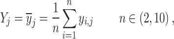
For each snRNA-seq dataset with annotated cell types, we randomly choose a subset of cells (2 < n < 10) to generate a simulated spatial spot. We defined the transcriptome profiles of the spot as the average gene expression of the selected n cells. In essence, we computed the mean expression level of genes across the n cells to formulate the transcriptome profiles of the simulated spot. That is,

where Y_j is the expression of gene j in a single simulated spatial spot, while = (, …), represents the expression of gene j in cell i. After iterating the process 1000 times, we generated 1000 simulated spots consisting of multiple cells. To access the impact of gene capture rates on various algorithms, we conducted down-sampling of gene counts at each of these 1000 spots to 1000, 2500, 5000, 10 000, 15 000 and 20 000 capture levels, respectively. The proportion of original cell types in each spot was recorded as a gold standard to demonstrate the accuracy of the deconvolution of algorithms.

Inspection methods

We employed three indexes to evaluate the performance of different mapping methods. Below are the specific criteria we have selected. Additionally, all subsequent vectors used are treated as column vectors. First, we intersected gene names of snRNA-seq data and ST data:

where represents the names of all genes in the snRNA-seq data, represents the names of all genes in the ST data and represents the names of the gene selected for all subsequent operations.

To proceed with the subsequent comparison, we first calculate the average gene expression for each cell type in the annotated snRNA-seq data:

where represents the average expression amount of the gene j under the cell type i, m represents the total number of cells under the cell type i and represents the expression amount of the gene j in the cell k under the cell type i. The column vector can be used to characterize the expression of the selected gene j in cell type i within snRNA-seq data because the obtained mapping result matrix represents the probability distribution of each cell type. To obtain the ST mapping result, we select the cell type with the highest probability, which is denoted by , indicating the gene j expression of all cells with the highest probability.

To reflect the similarity between the mapping results and the ground truth in a diverse and comprehensive manner, we have selected PPMCC and SSIM algorithms to represent the similarity. Similarly, to illustrate the variability between mapping results and real results, we used KL method for reference. These above indicators are then combined for an overall evaluation. The following are the specific calculation indicators:

Pearson product–moment correlation coefficient

We use PPMCC (Pearson product–moment correlation coefficient) to verify the correlation between mapping results and real gene spatial distribution. A higher PPMCC value indicates better mapping results. The main formula is as follows:

among them, represents the average expression of gene j of selected cell type in the result data, is the expression of gene j in real ST data, represents the average expression of gene j in the ST data, q represents the total number of selected differential genes, reflects the Pearson correlation between snRNA-seq data and ST data of this cell type, and represents the average Pearson correlation between snRNA-seq data and ST data under the selected mapping method.

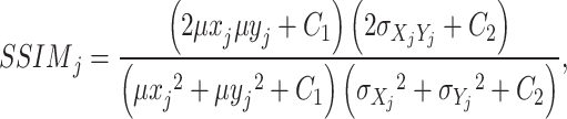
Structural similarity [33]

To characterize the structural similarity of data, we also use structural similarity as one of the methods to test the effect of mapping. The main formula is as follows:

Among them, reflects the structural similarity between snRNA-seq data and ST data of this cell type in terms of the distribution of gene j, and represents the overall structural similarity between snRNA-seq data and ST data under the selected mapping method.

Kullback–Leibler

KL (Kullback–Leibler) divergence is an indicator used to describe the difference between two probability distributions. The main formula is as follows:

where reflects the dispersion degree of snRNA-seq data and ST data of this type of cells in terms of the distribution of gene j, and represents the overall dispersion of snRNA-seq data and ST data under the selected mapping method.

Accuracy scoring system

In order to establish a comprehensive evaluation system, the respective rankings of the above three indicators are recorded as , and . At the same time, add a new indicator , which represents the number of identified cell types. We computed the average of PPMCC, KL and SSIM in all cell types predicted by each method, sorted the PPMCC, SSIM and TYPE in ascending and KL in descending order. Then, we add up the results from ranking four different indicators and normalize the sum to achieve an accuracy scoring system (ASS) score ranging from 0 to 1. The final ASS score is as follows:

Implementation of methods

SpatialDWLS: we used the code of SpatialDWLS from https://github.com/rdong08/spatialDWLS_dataset. We set the method = ‘scran’, expression_values = ‘normalized’, cluster_column = ‘leiden_clus’ for the ‘findMarkers_one_vs_all’ function and resolution = 0.4, n_iterations = 100 for ‘doLeidenCluster’ function.

RCTD: we used the code of RCTD from https://github.com/dmcable/spacexr, which is integrated into a tool called spacexr (2.0.0). We set doublet_mode = ‘full’. When processing the reference data, the ‘n_max_cells’ parameter is set to 10 000.

Seurat: we followed the instructions on the Seurat 3.2 website: https://satijalab.org/seurat/archive/v3.2/integration.html. We set the parameter dim = 1:30, normalization.method = ‘SCT’, reference.reduction = ‘pca’ for the ‘FindTransferAnchors’ function.

Tangram: we used the code of Tangram from https://github.com/broadinstitute/Tangram. We set the parameters as mode = ‘cells’, density_prior = ‘rna_count_based’, num_epochs = 100 for the ‘map_cells_to_space’ function.

Cell2location: we used the code of Cell2location from https://github.com/BayraktarLab/cell2location. The settings max_epochs = 250, batch_size = 2000, train_size = 1, lr = 0.002 were used for the train.

DestVI: we used the code of DestVI from https://github.com/scverse/scvi-tools. We set the parameters max_epochs = 250 when training the snRNA-seq model. The spatial model was trained for 2000 epochs, with a learning rate of 0.001.

Spatial-ID. We followed the instructions on the website: https://github.com/STOmics/SpatialID/tree/main/spatialid. When mapping labels from reference data to spatial data, we set the pca_dim = 200, k_graph = 30, edge_weight = True, epochs = 200, w_cls = 20, w_dae = 1 and w_gae = 1.

Spann: We followed the instructions on the website: https://github.com/ddb-qiwang/SPANN-torch. Then configured the perparameters as follows: learning rate was set to 2e-4, k_graph was set to 30, lambda_spa was set to 0.001, Lambda_recon was set to 200, and Lambda_kl was set to 0.5.

Uniport: We followed the instructions on the website: https://github.com/caokai1073/uniPort. During training, we employed a mode parameter value of 'h' and utilized a batch size of 256 to optimize training efficiency.

Results

Benchmarking framework and datasets overview

We devised a pipeline to evaluate the effectiveness of mapping methods on Stereo-seq data (Fig. 1A). In summary, we generated a pseudo-ST dataset with known cell-type identities using annotated snRNA-seq data. Subsequently, different algorithms were applied to annotate these labeled pseudo-ST datasets, and the disparities between the algorithmic annotations and the true labels were measured. Concurrently, we evaluated the performance of these algorithms on actual ST datasets from the mouse brain using metrics outlined in the Methods section.

Figure 1.

Benchmarking workflow and schematic overview of the ST datasets. (A) The benchmarking workflow demonstrated the evaluation of multiple mapping algorithms. The whole workflow can be divided roughly into two parts: the simulation comparison of snRNA-seq data and the mapping of real Stereo-seq ST data from four brain regions. (B) An overview of ST data obtained from four brain regions across two chips, including spot numbers, available genes and observed expression counts for each gene. OB: olfactory bulb; HIP: hippocampus; CTX: cortex; CB: cerebellum.

The Stereo-seq and snRNA-seq data were derived from our previously published or preprint work [30]. We collected eight paired datasets encompassing Stereo-seq and snRNA-seq data from four distinct mouse brain regions, including hippocampus (HIP), cerebellum (CB), olfactory bulb (OB) and cortex (CTX). These paired ST data and snRNA-seq data were derived from different mouse of the same strain and age. For the Stereo-seq data, we partitioned the quantified gene expression matrices derived from the four brain areas into bin50 size (50 × 50 DNB spots, dimension size: 25 μm × 25 μm), aggregating transcripts of identical genes within each bin. Subsequently, each bin50 was treated as a discrete spatial entity for subsequent analyses. Concurrently, cell segmentation was executed utilizing nucleic acid staining images obtained from the corresponding tissue sections, facilitating the acquisition of cellbin data by aligning these stained images onto the Stereo-seq chips (Fig. 1B). Compared with cellbin data, the bin50 data integrated transcript information from multiple cells, leading to both higher gene and UMI numbers than in cellbin data (Fig. 1B).

Comparison of multiple mapping algorithms on pseudo-ST data

We initially analyzed snRNA-seq data comprising 187,079 cells from four brain regions (Fig. 2A, B and Fig. S1A, available online at http://bib.oxfordjournals.org/). To visualize the two-dimensional distribution of these cells, we employed Uniform Manifold Approximation and Projection (UMAP). In HIP, cells were classified into 17 distinct cell types, whereas cells in CB were divided into 7 cell types (Fig. 2A and B). All these cell types were identified in our previous research [30]. The snRNA-seq data harvested from four brain regions were then used for simulations of the pseudo-ST data following the guidelines mentioned in the Methods, and the actual cell composition of each simulated spot was recorded as reference for annotating the simulated pseudo-ST datasets.

Figure 2.

Performance of six algorithms in pseudo-ST data. (A) UMAP visualization of hippocampal cell types. CA1/2/3 (Cornu Ammonis 1/2/3), DG (Dentate Gyrus), IN (inhibitory neurons), OPC (oligodendrocyte precursor cells), VLMC (vascular leptomeningeal cells). (B) UMAP visualization of cerebellar cell types. (C) The performance of six methods on the simulated dataset with varying gene numbers. Pearson’s correlation between the predicted proportions and the ground truth was calculated for each spot. CTX (cortex), HIP (hippocampus), CB (cerebellum), OB (olfactory Bulb). (D) Pearson’s correlation between the gene expression of predicted cell types and the ground truth was calculated for each cell types.

While annotating simulated pseudo-ST data from four brain regions, notable differences emerged among the various algorithms. In the spot-level correlation analysis, each point represented a simulated spot, and the y-axis of each point represented the Pearson correlation coefficient between the actual cell-type proportion and the algorithm-predicted cell proportion (Fig. 2C). RCTD demonstrated excellent mapping performance across all brain regions, with Cell2location following closely. However, not all these algorithms demonstrated stable performance across different brain regions. For example, Tangram and SpatialDWLS exhibited notably high correlation coefficients in the CB, but significantly lower correlation coefficients in other brain regions, including the HIP, CTX and OB. In principle, the mapping capabilities of these algorithms tended to be positively correlated with the number of captured genes. Nevertheless, exceptions were observed, such as the opposite trends observed with DestVI in the CB and Seurat in the CTX (Fig. 2C). This discrepancy may be attributed to either model overtraining or the initial random selection of key genes, where subsequent gene additions amplified the noise.

In the correlation analysis at the cell-type level, simulated spots were initially annotated by snRNA-seq data with the above six algorithms, respectively. The spots classified as same cell type were then aggregated together to obtain average expression level of gene in the predicted cell type. Correlation coefficient between gene expression of the actual cell type and the predicted cell type was calculated at the end (Fig. 2D). Cell-type level analysis aims to assess the similarity in gene expression between algorithm-annotated cell types and those identified in snRNA-seq data. In the HIP, for instance, the CA1 (CA, Cornu Ammonis) neurons predicted by RCTD in the simulated data exhibited the highest correlation coefficient (approximately 0.6) with the CA1 neurons in snRNA-seq data. Conversely, in the simulated data, the CA1 neurons predicted by Cell2location exhibited the lowest correlation coefficient in gene expression with CA1 neurons in snRNA-seq data. Cell2location and DestVI demonstrated lower correlation between predicted and actual cell type across all four brain regions in contrast to the other four mapping algorithms. Collectively, RCTD exhibited a better performance in simulated pseudo-ST data across four brain regions.

Algorithms’ performance in cell mapping across mouse brain regions

To accurately assess the performance of various mapping algorithms, we utilized cell-annotated snRNA-seq data obtained from the four brain regions as a reference to characterize cell identity in ST datasets. In the testing with real-world ST data, we incorporated additional algorithms, including those based on graph convolutional neural networks such as SpatialID, and those using optimal transport methods like Uniport and Spann.

For the HIP from adult sagittal brain section, spatial locations of all cell types predicted by the nine algorithms were shown (Fig. 3A). By comparing with the known anatomical structure of the HIP, we can evaluate the accuracy of the spatial distribution of the cells annotated by these algorithms. Notably, we found that RCTD and SpatialDWLS can correctly identified the major subregions of HIP, including DG (Dentate Gyrus), CA1, CA3 and even CA2 (colored in green in Fig. 3A). However, other algorithms were unable to delineate CA2 region. Uniport, Tangram and Cell2location could reconstruct the spatial distribution of major cell types in ST data, but their precision was relatively low, especially in terms of fuzzy boundaries and unclear demarcations between different regions. Lastly, Seurat, Spatial-ID, Spann and DestVI could only marginally distinguish between glial and neuronal regions, occasionally assigning incorrect cell identities to spatially distinct cell populations (Fig. 3A). All these algorithms demonstrated substantially differential mapping capabilities in HIP.

Figure 3.

Algorithm performance in ST data of the hippocampal region. (A) The spatial distribution of the cell types predicted by the algorithms, with colors representing different cell types. Astro (Astrocyte), CA1/2/3 (Cornu Ammonis 1/2/3), DG (Dentate Gyrus), IN (inhibitory neurons), OPC (oligodendrocyte precursor cells), VLMC (vascular leptomeningeal cells), Oligo (oligodendrocyte). (B) ASS score of the various algorithms, with colors representing different chips and the shades of color representing different resolutions. (C) The spot level correlation of the algorithms on simulated data, using a set number of genes at 2500. (D) The proportion of cell types in the reference data (snRNA-seq) and the proportion of cells predicted by algorithms in bin50 and cellbin datasets, respectively.

To quantify the accuracy of these algorithmic annotations, we constructed an ASS, which integrated various distance and correlation indicators. In the z-score results of ASS, RCTD and SpatialDWLS emerged as the top two algorithms, whereas Spatial-ID and DestVI were positioned as the bottom two algorithms (Fig. 3B). This result of the quantified scores was closely in line with our earlier anatomical-based assessments in Fig. 3(A). The quantified ASS scores, along with the spatial anatomical structure, illustrated that the performance of these algorithms across various datasets and replicates (bin50 versus cellbin, C2D2 versus C3D3) of the same brain region is consistent. These results suggested that ASS scores can accurately evaluate the performance of various algorithms in cell-type annotation. Meanwhile, we observed disparities in performance ranking of some algorithms in the simulation results compared to those based on the ASS score; however, RCTD consistently maintained excellent performance in both simulation results and ASS score evaluations (Fig. 3B and C). Subsequently, we compared the cell composition identified in the snRNA-seq dataset with the predictions made by algorithms (Fig. 3D). Our findings showed that Spatial-ID and DestVI only can label limited cell types whereas RCTD and SpatialDWLS, generally mimicked the cell-type composition observed in the snRNA-seq data. Certain cell types, such as DG neurons, were sparsely represented in the snRNA-seq data, but were still precisely mapped by RCTD and SpatialDWLS in DG of HIP. This may suggest that these two algorithms could effectively adjust the impact of distorted cell-type proportions in the snRNA-seq data. The comparison among Stereo-seq, Slide-seq and STARmap data revealed that RCTD exhibited strong mapping capabilities across all datasets. However, DestVI performed poorly in Stereo-seq and STARmap datasets but showed promising results in Slide-seq data (Fig. S2A and B, available online at http://bib.oxfordjournals.org/).

For CB, a parallel analysis was carried out as in HIP. Each cell/bin was assigned a cell-type label by the algorithm and mapped to its corresponding spatial location (Fig. 4A). ASS scores were subsequently calculated to evaluate the mapping outcomes for each algorithm. As anatomical structure of CB is stratified, this facilitated a straightforward comparison of the spatial distribution of various cell types among different algorithms. Regardless of the spatial distribution of various cell types or ASS evaluations, RCTD and SpatialDWLS remained the top-performing algorithms. These two algorithms successfully reconstructed the granule layer, Purkinje cell layer and molecular layer structures in the mouse CB with both bin50 and cellbin data. In contrast, the performance of other algorithms was relatively mediocre. Cell2location failed to identify the Purkinje cell layer and molecular layer, while Seurat, DestVI and Spatial-ID were unable to accurately re-construct spatial organization of molecular, Purkinje and granule cell layer in CB (Fig. 4A). From the HIP to the CB, the performance of Tangram was unstable. It could recognize basic anatomical structures in the HIP but was not the case in the CB, leading to a sharp decline in ASS scores from the top three to the bottom (Fig. 4A and B). In the simulated benchmarking, RCTD and SpatialDWLS consistently exhibited the highest correlation coefficients. However, the average correlation coefficient of Tangram, approaching 0.9, evidently did not reflect the real performance in CB. For cell composition in CB, the proportion of granule cells in the snRNA-seq data was much higher than that in the ST data annotated by RCTD and SpatialDWLS but was consistent with Seurat’s annotation results. As Seurat could not reconstruct granule cell layer as stated before, it seems that high similarity in cell composition with single-cell dataset was one of parameters to evaluate performance of various algorithms and more factors should be included for more precise assessment.

Figure 4.

Algorithm performance in ST data of the cerebellum region. (A) Spatial distribution of the cell types predicted by the nine algorithms. Astro (astrocyte), VLMC (vascular leptomeningeal cells), Oligo (oligodendrocyte). (B) ASS score of the nine algorithms. Colors represented different chips and the shades of color represented different resolutions. (C) Spot-level correlation of the algorithms on simulated data. The number of genes was set at 2500. (D) Proportion of cell types in the reference data (snRNA-seq) and the proportion of cells predicted by each algorithm.

In addition to the HIP and CB, we also analyzed ST data from the OB (Fig. S3, available online at http://bib.oxfordjournals.org/). In brief, among all the algorithms tested on ST data from these regions and two chips, RCTD appeared to be the top algorithm for cell mapping and annotation, even in simulation results.

Performance of ASS scores in practice

We employed various methods to comprehensively compare the results obtained by different algorithms and found that RCTD and SpatialDWLS might be the most suitable algorithms for annotating Stereo-seq data from mouse brain. Simultaneously, by integrating ASS scores from spatial datasets of multiple brain regions, including the HIP, CB and OB, we observed a consistent correlation between ASS scores and the actual performance of various algorithms (Fig. 5A). This demonstrated the capability of ASS scores system to select a suitable algorithm for cell mapping and annotation. Consequently, we established a framework for computing ASS scores for all algorithms involved in this study on ST datasets. To evaluate the performance of this framework, we utilized ST data from the mouse CTX along with corresponding snRNA-seq data as input for the framework. Additionally, we tested the robustness of the ASS framework by using mouse CTX snRNA-seq data from the 10X sequencing platform, assessing its performance when dealing with data from different platforms (Fig. 5B).

Figure 5.

Validation of ASS across different datasets. (A) The summary of ASS scores for different algorithms across the three brain regions. (B) UMAP visualization for snRNA-seq data from the mouse cortical region obtained from the 10X sequencing platform. Astro (astrocytes), Endo (endothelial cells), Micro (microglia), OPC (oligodendrocyte precursor cells), VLMC (vascular and leptomeningeal cells), OD (oligodendrocyte). (C) The line plot showing the ASS results for the annotation of the CTX using snRNA-seq data from the DNBelab C4 sequencing platform. (D) Spatial visualization showing the results annotated by RCTD and DestVI using DNBelab C4 snRNA-seq data. (E) The line plot showing the ASS results for the annotation of the CTX using snRNA-seq data from the 10X sequencing platform. (F) Spatial visualization showing the results annotated by RCTD and DestVI using 10X snRNA-seq data.

Consistent with previous test results in other brain regions, the ASS framework continued to rate high for RCTD in the CTX and low for DestVI (Fig. 5C). We then spatially visualized the annotation results of RCTD and DestVI in the CTX. Compared with DestVI, cell distribution pattern within CTX generated by RCTD was more similar with previous reports (Fig. 5D) [9, 31]. Interestingly, the ASS scores generated by the snRNA-seq datasets from different platforms were nearly identical (Fig. 5C and E). Spatial visualization of either bin50 or cellbin dataset showed a more detailed cortical layers from the 10X snRNA-seq. RCTD represented the clear six-layer structure from L1 to L6 in CTX. Although applied snRNA-seq dataset generated from different platform, the rankings of various algorithms still aligned with ASS scores (Fig. 5F). These results demonstrated that our proposed ASS framework performed well in selecting the best algorithm, even dealing with cross-platform data.

Discussion

This article discusses various prevalent spatial mapping algorithms employed for annotating cell types and independently evaluates the performance of these algorithms in annotating Stereo-seq ST data and pseudo-ST data. Utilizing ST data with single-cell resolution (e.g. seqFISH and MERFISH) for generation of pseudo-ST data may be more realistic [29]. However, it’s worth noting that image-based ST methods like MERFISH and STARmap have limitations in the total number of RNA transcripts. Additionally, none of the algorithms considered spatial location information in the analysis of simulated pseudo-ST data. Therefore, we adhered to the previous research strategy [28], employing snRNA-seq data to generate pseudo-ST data. The advantage of this simulation method is that the inherent cell-type composition of each simulated pseudo-ST spot is known in advance, providing a gold standard for assessing the accuracy of algorithmic annotation. In the evaluation of pseudo-ST data, RCTD demonstrated superior performance across all four brain regions. This was in line with the observations made by Chen et al. across three distinct ST datasets, despite not employing Stereo-seq [32]. While the simulation approach can assess the similarity of gene expression between the predicted and actual cell types, its primary limitation lies in overlooking the rationality of the spatial distribution of these cell types. This was illustrated in the simulation-based testing of the CB. Tangram exhibited very high correlation coefficients at both the cell type and spot levels (Fig. 2C and D). However, when applied to real CB ST data, Tangram’s results were entirely inaccurate in terms of spatial distribution (Fig. 4A). These findings highlighted issues with existing benchmarks, indicating that simulated data cannot fully substitute for real ST data in benchmark testing. Additionally, these results emphasized the pressing need for a method that can precisely evaluate the mapping capability in a real and genuine context.

The limitations of the simulation method prompted us to propose a novel evaluation metric named ASS, which amalgamated multiple indicators such as structural similarity, JS divergence and Pearson correlation coefficient. We previously observed that in statistics, a high numerical value or correlation coefficient doesn’t always equate to the biological relevance of structures or functions. Current peer-reviewed studies rely on the similarity and robustness of results to evaluate and rank various algorithms. However, whether these scores and rankings truly represent success in biology is uncertain. Here, through anatomical comparisons informed by experience and comprehensive assessments across multiple brain regions and resolutions, we have observed that the ASS score serves as an effective metric for evaluating algorithmic annotations from both statistical and biological standpoints. Integrating ASS scores with empirical assessments of cellular spatial distributions, we observed that RCTD and SpatialDWLS emerged as the most effective mapping methods for Stereo-seq data annotation in the mouse brain. This observation aligned with the comparative analysis of mouse cortical data conducted by Chen et al., where RCTD and SpatialDWLS were also recognized as top-performing methods for cell-type deconvolution of spots [28]. RCTD constructed based on probabilistic models combined with Poisson distributions and specially considered a gene-specific platform random effect. SpatialDWLS employed a weighted least squares approach to infer cell-type proportions, further optimizing them using enrichment analysis. These distinctive features might determine their applicability in the mapping of ST data. The superior algorithms enable the annotation of more detailed spatial structures and cell types, which greatly aids in exploring the potential biological phenomena underlying the data. For instance, within the spatial datasets of the mouse HIP, RCTD and SpatialDWLS can classify excitatory neurons into subtypes such as CA1, CA2, CA3 and DG neurons. In contrast, other algorithms that are somewhat less precise cannot annotate CA2 neurons. This distinction is crucial for researchers who focus on the molecular feature variations among different neuronal subtypes.

Our comparative analysis highlighted that the efficiency of these mapping methods in predicting cell types from ST data was notably influenced by the sparsity observed in both the ST expression matrix and the snRNA-seq expression matrix. This effect of matrix sparsity might be more pronounced for algorithms that rely on selecting the optimal gene subset from the snRNA-seq dataset as anchor points for feature matching, such as Tangram and DestVI. One observation is that, compared with the HIP and CTX, the matrices of the ST data in the CB and OB demonstrated higher sparsity, characterized by lower values of nFeature and nCounts. Consequently, Tangram’s annotation performance also showed a pronounced decline in the CB and OB. When the resolution of the ST data is increased from the spot level to the single-cell level, notable alterations occurred in the mapping results of DestVI and cell2location, suggesting that these algorithms were affected by drop-outs. Additionally, we compared the performance of different algorithms on Stereo-seq, Slide-seq and STARmap data. Compared with evaluations in peer studies [28, 29], which involved data from different platforms, tissue sources or even species, we believe our approach allows for an objective comparison of algorithms under more controlled conditions. The results revealed that algorithms may exhibit preferences for different ST methods, underscoring the necessity of conducting performance testing specifically on Stereo-seq data. Another potential application of this study is the direct selection of suitable mapping algorithms for different datasets through ASS, without relying on any judgment process based on prior knowledge. Through the analysis of snRNA-seq (10X and DNBelab C4) and ST datasets (Stereo-seq, Slide-seq and STARmap) from the different sequencing platforms, we demonstrated that the ASS framework reliably performed cross-platform optimal algorithm matching tasks. Due to the higher efficiency of capture gene transcripts in snRNA-seq as compared with ST data, most algorithms took advantage of snRNA-seq data to map cell types in ST data. Accordingly, we employed similar strategy and assumed that cell types in the ST data were all included in the snRNA-seq reference data; however, it could not completely rule out the possibility that novel or rare cell type was in ST data but missed in snRNA-seq because of technique bias. To overcome this, ST technique with capability of capturing more transcripts should be developed in future.

Key Points

• Mapping algorithms play a crucial role as the primary step in the current spatial transcriptomics data processing workflow, facilitating cell-type annotation in the context of limited gene capture rates and spot size.

• In a dual comparison based on simulation and real experiments on mouse brain data, we identified RCTD and SpatialDWLS as the optimal mapping algorithms for mouse brain Stereo-seq data.

• We propose a novel evaluation metric that accurately quantifies the mapping performance of cell types, allowing the selection of the most suitable mapping algorithm without any prior knowledge.

Author Biographies

Quyuan Tao is a PhD student at the School of Life Sciences, University of Chinese Academy of Sciences. His research interests include bioinformatics and deep learning with applications to brain science.

Yiheng Xu is a PhD student at the School of Medicine, Zhejiang University. His research focuses on various aspects of neuroscience, particularly its applications in artificial intelligence technologies.

Youzhe He is a postgraduate student at the School of Life Sciences, University of Chinese Academy of Sciences. His research interests include bioinformatics, deep learning and neuroscience.

Ting Luo is a postdoctoral researcher at BGI Research. Her research interests are bioinformatics and brain science.

XiaoMing Li is a professor at the School of Medicine, Zhejiang University. His research focuses on understanding the circuit and molecular mechanisms underlying the emotions and related disorders.

Lei Han is a principal scientist at BGI Research. His research focuses on integration and application of cell multi-omics data in brain development and disease.

Funding

The project was supported by National Science and Technology Innovation 2030 Major Program (Grant No. 2021ZD0204400).

Data availability

Custom code supporting the current study is available at https://github.com/qyTao185/Benchmarking-Mapping-Algorithms/tree/main. The processed 10X snRNA-seq datasets reported in this study can be available via NCBI’s Gene Expression Omnibus (GEO) Accession Number GSE190940. Processed h5ad files are available at https://github.com/shekharlab/mouseVC.The STARmap hippocampal data were obtained from Zenodo 562 (https://zenodo.org/records/8041114). Slide-seq hippocampal data were obtained from the Broad Institute Single Cell Portal 557 (https://singlecell.broadinstitute.org/single_cell/study/SCP948/robust-decomposition-of-cell-type-558 mixtures-in-spatial-transcriptomics). The raw data for the spatial transcriptome from Stereo-seq and snRNA-seq from DNBelab C4 can be accessed via https://doi.org/10.12412/BSDC.1699433096.20001.

References

- 1. Tasic B, Menon V, Nguyen TN, et al. Adult mouse cortical cell taxonomy revealed by single cell transcriptomics. Nat Neurosci 2016;19:335–46. [DOI] [PMC free article] [PubMed] [Google Scholar]
- 2. Zeisel A, Muñoz-Manchado AB, Codeluppi S, et al. Brain structure. Cell types in the mouse cortex and hippocampus revealed by single-cell RNA-seq. Science 2015;347:1138–42. [DOI] [PubMed] [Google Scholar]
- 3. Moses L, Pachter L. Museum of spatial transcriptomics. Nat Methods 2022;19:534–46. [DOI] [PubMed] [Google Scholar]
- 4. Rao A, Barkley D, França GS, Yanai I. Exploring tissue architecture using spatial transcriptomics. Nature 2021;596:211–20. [DOI] [PMC free article] [PubMed] [Google Scholar]
- 5. Maynard KR, Collado-Torres L, Weber LM, et al. Transcriptome-scale spatial gene expression in the human dorsolateral prefrontal cortex. Nat Neurosci 2021;24:425–36. [DOI] [PMC free article] [PubMed] [Google Scholar]
- 6. Rodriques SG, Stickels RR, Goeva A, et al. Slide-seq: a scalable technology for measuring genome-wide expression at high spatial resolution. Science 2019;363:1463–7. [DOI] [PMC free article] [PubMed] [Google Scholar]
- 7. Chen KH, Boettiger AN, Moffitt JR, et al. RNA imaging. Spatially resolved, highly multiplexed RNA profiling in single cells. Science 2015;348:aaa6090. [DOI] [PMC free article] [PubMed] [Google Scholar]
- 8. Wang X, Allen WE, Wright MA, et al. Three-dimensional intact-tissue sequencing of single-cell transcriptional states. Science 2018;361:eaat5691. [DOI] [PMC free article] [PubMed] [Google Scholar]
- 9. Chen A, Liao S, Cheng M, et al. Spatiotemporal transcriptomic atlas of mouse organogenesis using DNA nanoball-patterned arrays. Cell 2022;185:1777–1792.e21. [DOI] [PubMed] [Google Scholar]
- 10. Eng CL, Lawson M, Zhu Q, et al. Transcriptome-scale super-resolved imaging in tissues by RNA seqFISH. Nature 2019;568:235–9. [DOI] [PMC free article] [PubMed] [Google Scholar]
- 11. Codeluppi S, Borm LE, Zeisel A, et al. Spatial organization of the somatosensory cortex revealed by osmFISH. Nat Methods 2018;15:932–5. [DOI] [PubMed] [Google Scholar]
- 12. Liu Y, Yang M, Deng Y, et al. High-spatial-resolution multi-omics sequencing via deterministic barcoding in tissue. Cell 2020;183:1665–1681.e18. [DOI] [PMC free article] [PubMed] [Google Scholar]
- 13. Cho CS, Xi J, Si Y, et al. Microscopic examination of spatial transcriptome using Seq-scope. Cell 2021;184:3559–3572.e22. [DOI] [PMC free article] [PubMed] [Google Scholar]
- 14. Ke R, Mignardi M, Pacureanu A, et al. In situ sequencing for RNA analysis in preserved tissue and cells. Nat Methods 2013;10:857–60. [DOI] [PubMed] [Google Scholar]
- 15. Wei X, Fu S, Li H, et al. Single-cell Stereo-seq reveals induced progenitor cells involved in axolotl brain regeneration. Science 2022;377:eabp9444. [DOI] [PubMed] [Google Scholar]
- 16. Chen A, Sun Y, Lei Y, et al. Single-cell spatial transcriptome reveals cell-type organization in the macaque cortex. Cell 2023;186:3726–3743.e24. [DOI] [PubMed] [Google Scholar]
- 17. Kleshchevnikov V, Shmatko A, Dann E, et al. Cell2location maps fine-grained cell types in spatial transcriptomics. Nat Biotechnol 2022;40:661–71. [DOI] [PubMed] [Google Scholar]
- 18. Lopez R, Li B, Keren-Shaul H, et al. DestVI identifies continuums of cell types in spatial transcriptomics data. Nat Biotechnol 2022;40:1360–9. [DOI] [PMC free article] [PubMed] [Google Scholar]
- 19. Cable DM, Murray E, Zou LS, et al. Robust decomposition of cell type mixtures in spatial transcriptomics. Nat Biotechnol 2022;40:517–26. [DOI] [PMC free article] [PubMed] [Google Scholar]
- 20. Dong R, Yuan GC. SpatialDWLS: accurate deconvolution of spatial transcriptomic data. Genome Biol 2021;22:145. [DOI] [PMC free article] [PubMed] [Google Scholar]
- 21. Tsoucas D, Dong R, Chen H, et al. Accurate estimation of cell-type composition from gene expression data. Nat Commun 2019;10:2975. [DOI] [PMC free article] [PubMed] [Google Scholar]
- 22. Dries R, Zhu Q, Dong R, et al. Giotto: a toolbox for integrative analysis and visualization of spatial expression data. Genome Biol 2021;22:78. [DOI] [PMC free article] [PubMed] [Google Scholar]
- 23. Hao Y, Hao S, Andersen-Nissen E, et al. Integrated analysis of multimodal single-cell data. Cell 2021;184:3573–3587.e29. [DOI] [PMC free article] [PubMed] [Google Scholar]
- 24. Biancalani T, Scalia G, Buffoni L, et al. Deep learning and alignment of spatially resolved single-cell transcriptomes with tangram. Nat Methods 2021;18:1352–62. [DOI] [PMC free article] [PubMed] [Google Scholar]
- 25. Shen R, Liu L, Wu Z, et al. Spatial-ID: a cell typing method for spatially resolved transcriptomics via transfer learning and spatial embedding. Nat Commun 2022;13:7640. [DOI] [PMC free article] [PubMed] [Google Scholar]
- 26. Cao K, Gong Q, Hong Y, Wan L. A unified computational framework for single-cell data integration with optimal transport. Nat Commun 2022;13:7419. [DOI] [PMC free article] [PubMed] [Google Scholar]
- 27. Yuan M, Wan H, Wang Z, et al. SPANN: annotating single-cell resolution spatial transcriptome data with scRNA-seq data. Brief Bioinform 2024;25:bbab533. [DOI] [PMC free article] [PubMed] [Google Scholar]
- 28. Li B, Zhang W, Guo C, et al. Benchmarking spatial and single-cell transcriptomics integration methods for transcript distribution prediction and cell type deconvolution. Nat Methods 2022;19:662–70. [DOI] [PubMed] [Google Scholar]
- 29. Li H, Zhou J, Li Z, et al. A comprehensive benchmarking with practical guidelines for cellular deconvolution of spatial transcriptomics. Nat Commun 2023;14:1548. [DOI] [PMC free article] [PubMed] [Google Scholar]
- 30. Han L, Liu Z, Jing Z, et al. Spatially resolved molecular and cellular atlas of the mouse brain. bioRxiv2023.2012.2003.5695012023. 10.1101/2023.12.03.569501. [DOI]
- 31. Cheng S, Butrus S, Tan L, et al. Vision-dependent specification of cell types and function in the developing cortex. Cell 2022;185:311–327.e24. [DOI] [PMC free article] [PubMed] [Google Scholar]
- 32. Chen J, Liu W, Luo T, et al. A comprehensive comparison on cell-type composition inference for spatial transcriptomics data. Brief Bioinform 2022;23:bbac245. [DOI] [PMC free article] [PubMed] [Google Scholar]
- 33. Wang Z, Bovik AC, Sheikh HR, Simoncelli EP. Image quality assessment: from error visibility to structural similarity. IEEE Trans Image Process 2004;13:600–12. [DOI] [PubMed] [Google Scholar]
Associated Data
This section collects any data citations, data availability statements, or supplementary materials included in this article.
Supplementary Materials
Data Availability Statement