SpaNCMG: improving spatial domains identification of spatial transcriptomics using neighborhood-complementary mixed-view graph convolutional network

Abstract

The advancement of spatial transcriptomics (ST) technology contributes to a more profound comprehension of the spatial properties of gene expression within tissues. However, due to challenges of high dimensionality, pronounced noise and dynamic limitations in ST data, the integration of gene expression and spatial information to accurately identify spatial domains remains challenging. This paper proposes a SpaNCMG algorithm for the purpose of achieving precise spatial domain description and localization based on a neighborhood-complementary mixed-view graph convolutional network. The algorithm enables better adaptation to ST data at different resolutions by integrating the local information from KNN and the global structure from r-radius into a complementary neighborhood graph. It also introduces an attention mechanism to achieve adaptive fusion of different reconstructed expressions, and utilizes KPCA method for dimensionality reduction. The application of SpaNCMG on five datasets from four sequencing platforms demonstrates superior performance to eight existing advanced methods. Specifically, the algorithm achieved highest ARI accuracies of 0.63 and 0.52 on the datasets of the human dorsolateral prefrontal cortex and mouse somatosensory cortex, respectively. It accurately identified the spatial locations of marker genes in the mouse olfactory bulb tissue and inferred the biological functions of different regions. When handling larger datasets such as mouse embryos, the SpaNCMG not only identified the main tissue structures but also explored unlabeled domains. Overall, the good generalization ability and scalability of SpaNCMG make it an outstanding tool for understanding tissue structure and disease mechanisms. Our codes are available at https://github.com/ZhihaoSi/SpaNCMG.

Introduction

The normal function of cells and tissues is closely linked to the regulation of gene expression. Investigating the characteristics of gene expression within cells and tissues is essential for unraveling the complex regulatory networks within an organism [1, 2]. Spatial transcriptomics (ST) technology allows for precise localization of gene expression while maintaining the integrity of tissue structure [3]. Various ST technologies differ in sequencing methods and are mainly classified into two categories [4, 5]: imaging-based (e.g. MERFISH [6], seqFISH+ [7], and osmFISH [8]) and sequencing-based technologies (e.g. 10x Visium [9], Slide-seq [10], and Stereo-seq [11]). Precise identification of spatial domains is a key step in analyzing ST data. The identification and analysis of gene expression patterns in different spatial regions of tissues facilitates the elucidation of the spatial positions and interrelationships of different cell types within the tissue structure. Additionally, the accurate identification of spatial domains also plays an important role in the onset and progression of diseases [12].

The early classical spatial domain identification methods (e.g. Spaniel [13], Seurat (V3.2) [14], spatialLIBD [15], and SpatialCpie [16]) that rely solely on gene expression information result in less than ideal identification performance. While the recent algorithms have started to integrate spatial locations to improve clustering accuracy. For example, through the use of generative methods, BayesSpace [17], Giotto [18], and SC-MEB [19] use traditional probability models to decrypt the spatial domain. However, the performance of these methods is still limited in handling large-scale ST data. With the advancement of deep learning, it becomes a powerful tool for analyzing spatial domains [20]. In application, stLearn [21] introduces deep learning models to extract image features and combines them with spatial location and gene expression. SEDR [22] uses deep autoencoders to construct low-dimensional latent representations of gene expression. SpaGCN [23] fuses gene expression and spatial location through graph convolution techniques to identify spatial domains with consistent representations. conST [24] effectively integrates multimodal data using a deep learning framework to learn low-dimensional latent embeddings for downstream clustering analysis. CCST [25] uses deep graph neural networks to perform clustering with ST data. Although the spatial structure of ST is considered, the current algorithms have limitations in capturing spatial neighborhood information. This is because they rely on fixed similarity measures, which makes it difficult to adapt to ST data at different resolutions and fully utilize neighborhood information. As a result, it limits the spatial domain recognition capability of the algorithms. Furthermore, when integrating reconstructed gene expression, traditional models use a simple additive approach which fails to adaptively fuse key information. This reduces the overall data quality and interpretability of the model. In terms of unsupervised clustering, traditional PCA dimensionality reduction can indeed remove some redundant features. However, when dealing with complex ST data, it might overlook critical nonlinear features, which potentially impact clustering performance.

To overcome the aforementioned challenges, we propose SpaNCMG to accurately identify Spatial domains by utilizing Neighborhood-Complementary Mixed-view Graph convolutional networks. This algorithm constructs neighborhood graphs using the KNN and -radius strategy, thereby enhancing the adaptability and accuracy of neighborhood definitions. By incorporating an attention mechanism to adaptively fuse various reconstructed gene expressions, the algorithm significantly boosts the model’s ability to capture key gene expression patterns and enhances the interpretability of predictive results. Furthermore, using the KPCA method for dimensionality reduction before clustering allows for a more effective representation of the complex relationships within the data. Experimental results indicated that SpaNCMG outperformed eight current advanced algorithms in spatial domain recognition. SpaNCMG exhibited robust clustering capabilities in both the human dorsolateral prefrontal cortex dataset and the mouse somatosensory cortex dataset. It accurately delineated tissue regions and inferred biological functions in the mouse olfactory bulb tissues. When dealing with large datasets such as embryo data, it can not only provide a more in-depth analysis of spatial structure within tissues but also identify domains that were previously unrecognized. In terms of generalization capability across different ST technologies, SpaNCMG proves to be a flexible analytical framework that can be extended to handle data from various platforms.

Materials and methods

Data preprocessing

To verify the clustering effect of the model, we use five datasets from four different platforms:

• (1) The first dataset is obtained from 10x Visium (http://research.libd.org/spatialLIBD/) and focuses on the human dorsolateral prefrontal cortex (DLPFC) with a resolution of 55 .

• (2) The second group is mouse somatosensory cortex dataset with subcellular resolution obtained from osmFISH (http://linnarssonlab.org/osmFISH/).

• (3) The third dataset is the Puck_200127_15 slices of a mouse olfactory bulb dataset obtained from Slide-seqV2 (https://singlecell.broadinstitute.org/single_cell/study/SCP815/highly-sensitive-spatial-transcriptomics-at-near-cellular-resolution-with-slide-seqv2#study-summary), with a resolution of 10 .

• (4) The fourth group is the mouse olfactory bulb dataset obtained from Stereo-seq, with a resolution of 220  (https://github.com/JinmiaoChenLab/SEDR_analyses/).

• (5) The final dataset is Stereo-seq acquired datasets of mouse embryos at E9.5 (https://db.cngb.org/stomics/mosta/).

For the raw gene expression data, we select the top 3000 highly variable genes (HVGs) as input and standardize them based on the library size. Subsequently, a natural logarithm transformation with base is performed. As the mouse somatosensory cortex dataset contains only 33 genes, this dataset retains all the genes.

Construction of spatial neighborhood network

K-Nearest Neighbor (KNN) [26] is adept at capturing the local structure of data [27]. The r-radius [28, 29] method is not confined to a fixed number of KNNs and can adapt to data with varying densities and distributions. It aids in revealing the global structure of the data [30]. To maximize the utilization of the similarity between adjacent spots, this study concurrently constructed two undirected neighborhood graphs , using both the KNN and the r-radius methods. Here, V represents the set of spots, represents the set of connecting edges between spots in the th graph, where represents the number of graphs. is defined as the adjacency matrix of graph , where N is the total number of spots. In the KNN method, if spots and are within each other’s KNNs, then , and 0 otherwise. Similarly, in the -radius method, if spots and are both within a pre-defined radius, then , and 0 otherwise. The selection of different parameters can affect the features of the central spots. The settings of the nearest neighbors and the radius are adjusted based on the resolution of the data, but both control the capture of spots within a range of 3–15.

In order to make the adjacency matrix more suitable for the Graph Convolutional Network and to avoid numerical explosion or vanishing during the feature propagation process, the adjacency matrix needs to be normalized before convolution to balance the influence between different spots. The normalized is obtained as follows:

(1)

(2)

where . Here, is the adjacency matrix with an additional self-connection, is the identity matrix. For the subsequent training of the graph convolutional network, the final neighborhood graph constructed integrates both gene expression information and spatial position information .

Data augmentation

Taking the graph constructed with as input, we train the model to extract spot features without altering the graph structure. We need to generate corrupted neighborhood graphs through data augmentation for contrastive learning. Specifically, on the originally constructed neighborhood graphs , we generate corrupted neighborhood graphs by randomly shuffling the gene expression vectors. This process shuffles the gene expression data while preserving the topological structure of the original neighborhood graph. This represents the shuffled gene expression profile.

Neighborhood-complementary multi-view graph convolutional networks

For this module of the model, we regard it as a multi-view graph convolutional network learning framework with an encoder and decoder. The encoder takes the neighborhood graph constructed from our preprocessed gene expression matrix as input to obtain the latent feature representation . The output of the encoder serves as the input to the decoder to obtain the reconstructed gene expression matrix . Specifically, in the encoder part, we consider a multi-layer graph convolutional network [31], where the propagation rule for the lth layer is as follows:

(3)

where is a trainable weight matrix, is a trainable bias vector and is the nonlinear activation function. is the output of the lth layer of undirected graph , with the initial represented by the gene expression matrix X (X, where N is the number of spots and D is the number of genes). The resulting latent feature representation is used as input and passed to the subsequent decoder to reverse back to the original feature space, resulting in the reconstructed gene expression matrix. The output of the tth layer for the reconstructed gene expression is formed as follows:

(4)

where , and represent the trainable weight matrix and bias vector in the decoder, respectively. In the training stage, we set the learning rate lr = 0.001 and the weight decay parameter weight_decay = 0.0001.

Self-reconstruction loss and self-supervised contrastive learning

To ensure that the final reconstructed gene expression H encompasses the majority of the overall information, we fully utilize the gene expression profiles to build a self-reconstruction loss model with minimization normalization, as follows:

(5)

The overall framework of our model is implemented based on Deep Graph Infomax (DGI) frameworks [32], which is a general method for learning node representations in graph-structured data in an unsupervised manner. It aims to maximize the mutual information (MI) between local representations and corresponding graph overview representations. In the DGI architecture, to ensure the model captures the local context information of the spots, the MI of positive examples is maximized:

(6)

where = . The discriminator is a function that distinguishes positive and negative examples by maximizing the probability of positive examples while minimizing the probability of negative examples. It is established for adversarial training. F represents the number of feature dimensions of spot . represents the microenvironment of spot , including gene expression information and spatial neighborhood information. However, to make the overall model more discriminative and balanced, the MI of Jensen–Shannon divergence maximization counterexamples is also used here:

(7)

Thus, the model is trained through self-reconstructive loss and self-supervised contrastive learning, ensuring its efficiency and accuracy. The total training loss is as follows:

(8)

where and are the loss weights. Based on experience, we set, .

Mix-reconstructed feature fusion

In the process of feature fusion, the attention mechanism focuses more on relevant information in the input and reduces attention on irrelevant details [33]. Unlike other attention mechanisms, we employ a soft-attention mechanism that is more capable of considering all input information during computation and assigning weights to each part. This mechanism not only integrates global contextual information but also takes into account all relevant information during output, making it comprehensive and easy to implement. Here, we apply the attention mechanism based on the importance of embeddings to the fusion of the reconstructed gene expression matrix , resulting in the final reconstructed gene expression matrix H. The main process of attention mechanism fusion is as follows:

(9)

Here, and are trainable attention coefficients, obtained through the attention mechanism:

(10)

(11)

where is the importance score of spot i, through a small neural network study. . is an alignment model (feed-forward neural network), also known as the scoring function. is a matching feature vector for interaction with the context. is transformed into probability form via , making represent the proportion of attention allocated to spot i. It is used to measure the relative importance of within ( is the vector corresponding to spot i in the reconstructed gene expression ). Let diag, we can determine the global information weights and , which are used to compute the final reconstructed gene expression matrix H.

Clustering

For data with a ground truth, such as 10x Visium and osmFISH, we employ the mclust [34] method. This approach leverages finite Gaussian mixture models, which confers a more robust statistical foundation. With prior knowledge, the data can be considered as consisting of multiple finite normal distributions. The mclust flexibly fits these mixture models to discern distinct gene expression patterns, thereby offering more precise classification results [35]. Its implementation primarily relies on the mclust package in R platform. Before clustering, we choose KPCA method to reduce dimension and remove some redundant features. For data without known ground truth such as Slide-seqV2 and Stereo-seq, we utilize the Louvain method in SCANPY [36]. In cases where the true segmentation of such data is not clear, our aim is to explore potential patterns within the data without being constrained by prior assumptions. Compared to the Leiden algorithm, Louvain is simpler and faster, effectively reducing running time on large datasets [37].

Evaluation index

For datasets with ground truth, we use the adjusted rand index (ARI) to evaluate the clustering results of model. ARI is insensitive to the number of clusters, allowing for a stable assessment of clustering quality [38]. Let U represent the actual classification and C represent the clustering results. Let a be the number of objects in the same class in U and also in the same class in C. Let b be the number of objects in the same class in U but not in the same class in C. Define ARI as follows:

(12)

(13)

Here, RI is the rand index, and is the expected value of the RI. For data without a ground truth, we directly observe the clustering results using visualization.

Uniform manifold approximation and projection analysis

Uniform manifold approximation and projection (UMAP) is an algorithm commonly used for dimensionality reduction of high-dimensional data, enabling the mapping of such data to a lower-dimensional space [39]. Generally, the high density and clear boundaries between clusters within the UMAP visualization indirectly that the algorithm has successfully captured the structural information in the data. The comparison of UMAP visualizations from different algorithms can indicate their relative effectiveness.

Ablation study

To further investigate the complementarity of the two strategies in the model of spatial domains identification, we conducted ablation studies on DLPFC and osmFISH datasets with ground truth. As shown in Fig. S1, we designed two variants of the SpaNCMG model. The first variant only used an r-radius similarity metric (without KNN, non-K) to identify neighboring points, while the other one only used the KNN technique (without r-radius, non-R) to capture neighborhood information. To ensure the fairness of the experimental results, all other parameters settings of model were kept consistent.

Results

Overview of SpaNCMG

SpaNCMG is a novel computational method to identify Spatial domains based on the Neighborhood-Complementary Mixed-view Graph convolutional network. SpaNCMG integrates gene expression profiles and spatial positional information as the overall embedding of the model (Fig. 1A). Gene expression information is obtained from spatial transcriptomic data, pre-processed to yield . To fully explore neighborhood information, SpaNCMG first utilizes the KNN and -radius similarity measurement methods to simultaneously construct the normalized adjacency matrix from spatial positional information, capturing the neighborhood spots for each data spot. Next, the pre-processed gene expression matrix and the adjacency matrix are jointly inputted into the neighborhood-complementary multi-view graph convolutional network (Fig. 1B). To enhance the training capabilities of the model, data augmentation is performed. Since different similarity measurement methods capture distinct spatial information, the neighborhood graphs obtained from each method are independently trained during the feature extraction phase.

Figure 1.

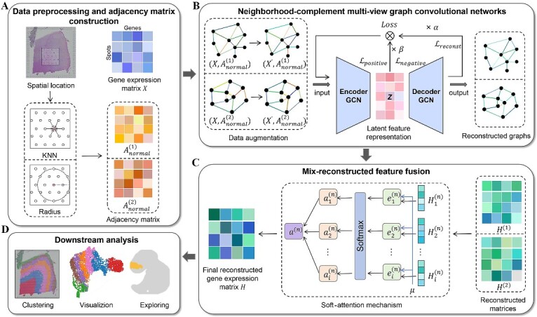
The overall workflow of SpaNCMG. (A) Data preprocessing and the construction of different spatial adjacency matrices with normalization. (B) Neighborhood-complementary multi-view graph convolutional network for feature training of different complementary neighborhood graphs, outputting the reconstructed feature graphs. (C) The reconstruction matrices mapped from the reconstructed feature graphs of (B) is fused through attention mechanism to obtain the final reconstructed gene expression. (D) The final reconstructed gene expression matrix’s biological applications.

With the constraints of training iterations and learning rates, the model performance is optimized by minimizing the overall loss consisting of the self-reconstruction loss and self-supervised contrastive learning loss. Through iterative training of the encoder, gene expression profiles and spatial location information are embedded into the latent representation space, yielding latent feature representation Z. After training the decoder, the latent feature representation is reversed back into the original feature space. By mapping the graph information to matrices, we obtain the reconstructed gene expression matrices and containing local and global information, respectively (Fig. 1C). Then, we employ an attention mechanism to integrate different similarity measurement methods and obtain a gene expression matrix containing a complete set of features. Based on the importance of the embeddings, this mechanism can adaptively combine the reconstructed gene expression matrices to obtain the final reconstructed gene expression matrix H. The final matrix provides a more robust and comprehensive representation of the gene expressions, and can be used for downstream clustering, UMAP visualization and detection of unlabeled areas (Fig. 1D).

SpaNCMG divides the spatial distribution patterns of known layers in the 10x Visium human dorsolateral prefrontal cortex

To evaluate the spatial domain recognition performance of SpaNCMG, we first applied it to the 10x Visium human dorsolateral prefrontal cortex (DLPFC) dataset with known. This dataset comprises 12 slices. The application of the DLPFC dataset with label information to spatial domain recognition allows for a quantitative evaluation of the algorithm’s potential application in handling complex tissue structures. To illustrate the model’s clustering capabilities, we compared it with eight recently developed spatial clustering methods (i.e. Seurat [40], SCANPY [36], conST [24], STAGATE [41], SEDR [22], SpaGCN [23], stLearn [21] and CCST [25]). Across all 12 slices, SpaNCMG achieved the highest median and average score among all methods (Fig. 2B). This method also surpassed the other two variants (Fig. S1), reflecting the enhanced ability of the combined method to recognize spatial domains in the DLPFC dataset.

Figure 2.

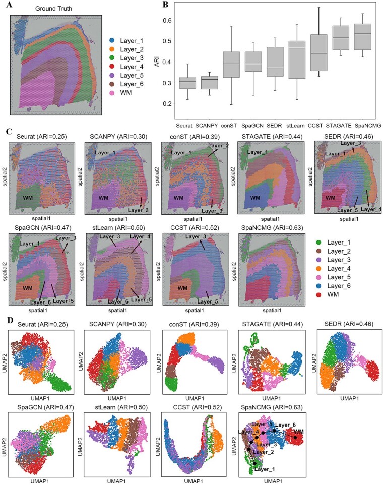
Spatial domain identification of the human dorsolateral prefrontal cortex by SpaNCMG. (A) Ground-truth segmentation of the slice 151675 of the DLPFC dataset. (B) Box plots of ARI scores for 12 slices of DLPFC using nine different methods. (C) Visualization of spatial domain recognition results on slice 151675 slices by nine different methods. (D) Visualization of UMAP plots generated by the nine different methods.

To further investigate the effectiveness of SpaNCMG in dividing spatial domains, we listed the recognition results on the slice 151675 of DLPFC, which consists of six cortical layers and a WM layer (Fig. 2A, C). Here, the confused identification results of some algorithms made it difficult to distinguish different regions, thereby we only annotated the partition results of SpaNCMG. Specifically, the segmentation results of Seurat and SCANPY were the poorest with unclear boundaries. The spots identified by conST, SpaGCN, and SEDR were too clustered between Layer_2 and Layer_6, lacking clear separation. The recognition results of STAGATE and CCST were clear and smooth in the regional boundary, but they erroneously merged several intermediate layers. On the original 151675 slice, the regions of Layer_2 and Layer_4 were relatively small, making them difficult to identify clearly. None of the other comparative methods managed to detect these two regions, whereas SpaNCMG achieved precise localization. In contrast, SpaNCMG’s identification was more aligned with the ground truth, achieving the highest ARI score of 0.63.

In UMAP visualization analysis, the results of Seurat, SCANPY, SpaGCN, and CCST were the most chaotic, lacking clear separation between clusters. Although the results of conST, STAGATE, SEDR, and stLearn had clear boundaries of clustered spots at various levels, they lost the order between regions and broke the original layered structure. In contrast, the UMAP plot of SpaNCMG not only exhibited distinct partitioning of clusters in each domain but also demonstrated a very clear sequential relationship between layers (Fig. 2D). These results demonstrated SpaNCMG’s superiority in identifying spatial domains within the 10x Visium DLPFC dataset, showcasing its exceptional clustering performance.

SpaNCMG’s spatial clustering on the osmFISH mouse somatosensory cortex dataset improved the recognition of known layers

The mouse somatosensory cortex dataset from osmFISH includes a variety of cell types, such as neurons and glial cells. It reveals the molecular characteristics and spatial organization of different cell types within the brain. This dataset can assist in evaluating the performance of algorithms when dealing with complex and heterogeneous data, and verify the robustness of algorithms. The selected observational domain contained 3405 cells with 33 genes, and its ground truth schematic was shown in Fig. 3(A). Due to the data incompatibility, we were unable to use the stLearn and Seurat methods, and instead compared the remaining six methods. In the comparative analysis, SpaNCMG achieved the highest score with an ARI of 0.52. Conversely, the other five methods yielded ARIs below 0.5 (Fig. 3B). The results of the ablation study showed that ARI values of non-K and non-R variants were significantly lower than SpaNCMG, indicating the effectiveness of the combined method (Fig. S1B).

Figure 3.

Spatial domain identification on the osmFISH mouse somatosensory cortex dataset using SpaNCMG. (A) Manual annotation of the layered structure in the mouse somatosensory cortex dataset. (B) Bar chart of ARI scores for seven methods. (C) Visualization of spatial domain identification results on the mouse somatosensory cortex using seven different methods. (D) Visualization of UMAP plots generated by the seven different methods.

The visualization analysis revealed that the cell distributions identified by SpaGCN, SEDR, SCANPY and conST were scattered and did not form clear underlying partitions (Fig. 3C). CCST displayed discontinuous clustering boundaries at the regions of Pia Layer 1 and Layer 6 with numerous misclassified cells. In contrast, both STAGATE and SpaNCMG exhibited efficient partitioning of the boundary regions of Pia Layer 1, Layer 6 and the internal Layer 2–3 regions. Additionally, the SpaNCMG successfully identified the Layer 4 region. We also visualized the embeddings generated by the dataset using UMAP (Fig. 3D). The UMAP visualizations of SpaGCN, SCANPY and CCST were the most cluttered with spots scattered across different regions. In contrast, the UMAP mappings of SEDR, conST, STAGATE and SpaNCMG resulted in comparatively clear demarcations. Among these, SpaNCMG effectively segregated the mapping of clusters associated with Layer 2–3, Layer 6 and Pia Layer 1. Combining the results from Fig. 3(B), we observed that SEDR and conST exhibit significant confusion in clustering identification, whereas the mapping in the UMAP embeddings was much clearer. Since UMAP represent the results of dimensionality reduction from high-dimensional data, we conjecture that SEDR and conST algorithms might struggle to learn effective feature representations for discerning various regions, consequently resulting in inferior clustering results after training.

Overall, SpaNCMG demonstrates superior clustering performance compared to other strategies and achieves relatively clean partition in UMAP visualization. These findings indicated that SpaNCMG performs well in identifying spatial domains in the osmFISH mouse somatosensory cortex dataset, exhibiting superior performance.

SpaNCMG revealed laminar flow structure of mouse olfactory bulb data from Slid-seqV2 and Stereo-seq and inferred biological function

The Slide-seqV2 and Stereo-seq technologies provide extremely detailed spatial and molecular data in the spatial transcriptomic study of the mouse olfactory bulb (MOB). Identifying the complex laminar tissue structure of the MOB can test the unraveling ability of the model in exploring new biological phenomena and patterns. To compare the recognition capabilities, 4 methods of SCANPY, SEDR, STAGATE, and SpaNCMG were used on tissue regions of MOB datasets acquired with Slide-seqV2 and Stereo-seq techniques at different resolutions.

We first evaluated the clustering performance of SpaNCMG on dataset acquired with Slide-seqV2. As illustrated in Fig. 4(A), employed the annotated Allen Brain Atlas as a reference [42]. By combining DAPI-stained images [22], the multiple structural layers of the mouse olfactory bulb were clearly discernible. In spatial domain recognition of the MOB dataset acquired with Slide-seqV2, it was evident that the regions identified by SpaNCMG closely aligned with annotations from the Allen Atlas (Fig. 4B). Both SCANPY and SEDR exhibited issues with blurred boundaries and unclear partitions. In contrast, STAGATE and SpaNCMG achieved obvious partitioning (Fig. S2A). Although STAGATE identified more regions, it failed to achieve clear clustering of the granule cell layer (GCL) domain internally. The regions identified by SpaNCMG aligned with the precise localization of marker genes (Fig. 4E), which also shows the accuracy of SpaNCMG recognition. To further elucidate the characteristics of the identified regions, we corresponded the recognition region to the marker gene. Referring to the Human Protein Atlas (https://www.proteinatlas.org/), we learned that the Pcp4 gene is a calcium-binding protein modulator involved in the calmodulin-dependent kinase signaling pathway and positive regulation of neuronal differentiation, and predominantly enriched in the GCL near the accessory olfactory bulb domain. This suggested that the GCL domain may play a crucial role in neuronal differentiation. Scg2 is highly expressed in the external plexiform layer (EPL) and mainly involved in the secretory protein family within neurons, regulating the biogenesis of secretory granules. Based on this, we inferred that the EPL layer may be associated with secretory regulation. For other identified domains, we can also investigate their potential biological functions using corresponding marker genes.

Figure 4.

Spatial domain identification in mouse olfactory bulb tissue using SpaNCMG. (A) Annotation of mouse olfactory bulb tissue from the Allen reference atlas. (B) Visualization of spatial domain identification results on Slide-seqV2 mouse olfactory bulb tissue using SCANPY, SEDR, and SpaNCMG. (C) Annotation of mouse olfactory bulb tissue in DAPI-stained images. (D) Visualization of spatial domain identification results on Stereo-seq mouse olfactory bulb tissue using SCANPY, SEDR and SpaNCMG. (E, F) Visualization of individual domains identified by SpaNCMG in mouse olfactory bulb tissue using Slide-seqV2 and Stereo-seq, along with the corresponding expression of marker genes.

In addition, we also examined the clustering performance of SpaNCMG on Stereo-seq MOB data. The naming conventions for different regions in Stereo-seq aligned with those in Slide-seqV2 (Fig. 4C). Compared to the SCANPY method, the three methods of SEDR, STAGATE and SpaNCMG can more accurately reflect the laminar structure of the MOB and align better with annotations in the DAPI-stained images produced by Stereo-seq (Figs 4D and S2B). Although SEDR divided the region into seven layers, it failed to associate its identified region 6 with any region in the stained images and did not recognize the narrow tissue structure glomerular layer. STAGATE segmented the MOB tissue into six regions with most regions being accurately identified, but the internal rostral migratory stream was not effectively identified. In terms of regional integrity, SpaNCMG excelled by dividing all seven layers, aligning closely with the regions depicted in the DAPI-stained images. Furthermore, we validated our clustering spatial domain results by exploring the expression locations of marker genes related to these regions (Fig. 4F). The olfactory nerve layer (ONL) domain corresponded to the expression domain of the Apod gene. According to the Human Protein Atlas, the Apod is involved in encoding a component of high-density lipoproteins. We speculated that the ONL domain might be related to lipoprotein metabolism. Gabra1 is a major inhibitory neurotransmitter in the mammalian brain and associated with certain diseases, and the mutations in this gene can lead to epilepsy. Thus, we hypothesized that the mitral cell layer might be related to epileptic seizures.

In summary, these results not only demonstrate SpaNCMG’s capability in handling different resolution tissue structures within the same region but also infer potential tissue functions through identified spatial domains. This provides vital references for subsequent research and exploration for organizational structure and function, and aids in uncovering deeper layers of biological information.

SpaNCMG’s spatial clustering on Stereo-seq mouse embryo dataset identified unlabeled tissue structures

Given the diversity of embryonic structures and the complex dynamics of gene expression among different tissues during their development (e.g. organ formation, cell migration and differentiation), the embryo data became an ideal choice for evaluating the model’s accuracy, robustness and biological interpretability. The employed E9.5 dataset contains 5913 bins and 25 568 genes. Owing to the lack of tissue descriptions in the Stereo-seq E9.5 mouse embryo dataset, we consulted the annotations for E9.5 in the MOSTA database [11] (https://db.cngb.org/stomics/mosta/), establishing a basic partition reference (Fig. 5A). Based on these annotations, the E9.5 mouse embryo dataset was divided into 12 distinct regions. To achieve more precise identification of small tissue regions, we set the number of clusters to 22. Considering the computational limitations of other algorithms, this paper only compares the SEDR, SCANPY, and STAGATE methods. Although the boundaries identified by STAGATE were smooth and clear, they were vaguely located in the heart without depicting the cavity within, and the method failed to recognize the surrounding lung tissue (Fig. S2C). The results of SEDR showed many clusters along the boundary regions, forming an outer layer (Fig. 5B). Similarly, SCNAPY’s results revealed a thick layer around the neural crest and the brain, which did not align well with the annotations.

Figure 5.

Spatial domain identification on Stereo-seq mouse embryo dataset using SpaNCMG. (A) Regional annotation of E9.5 mouse embryo tissue in the MOSTA database. (B) Visualization of spatial domain identification results on E9.5 mouse embryo dataset using SEDR, SCANPY, and SpaNCMG. (C) Visualization of partial individual domain identification results by SpaNCMG on E9.5 mouse embryo dataset. (D) Visualization results of corresponding marker gene expression for identified domains on the mouse embryo.

In contrast, the segmentation of SpaNCMG in both boundary regions and internal tissues was more consistent with annotations. The identified clusters (e.g. the heart, sclerotome and lungs) matched well with the expression of relevant marker genes (Fig. 5C, D), confirming the accuracy of SpaNCMG’s localization. Unlike the original annotation, the SpaNCMG divided the heart into two parts. Specifically, the Actn2 gene covered the entire heart, while the Nppa marker localized to the lower left part of the heart, confirming SpaNCMG’s delineation (Fig. 5D). The notochord is a unique embryonic region that appears transiently during the embryonic stage and gradually disappears as early brain development completes [43]. Although this area is small and not easily noticeable in the original annotation, SpaNCMG can effectively detect it. Additionally, the initial annotations marked a large area as the mouse brain, but SpaNCMG precisely located the telencephalon within it. The accuracy of the positioning was confirmed by the verification of the Lhx2 marker gene. SpaNCMG also discovered the branchial arch region, which is an important structure formed during the development of vertebrate embryos and is closely related to the development of head structures such as gills and jaws. Notably, no single marker gene can precisely locate this area, but it can be effectively identified under the combined expression of Msx1, Msx2 and Prrx1 marker genes [44].

Taken together, the clustering results on the E9.5 mouse embryo dataset effectively demonstrate the significant advantages of SpaNCMG in spatial domain recognition. SpaNCMG provides precise dissection of detailed hierarchical structures, confirming its robust capability in analyzing spatial expression patterns of complex biological processes. This capability not only offers a new perspective for understanding complex biological processes but also opens up new avenues for future biomedical research.

Discussion

As the fundamental and critical initial step in spatial transcriptome data analysis, accurately decoding the spatial domain is crucial for describing genomic heterogeneity and cell interactions. Here, we propose a spatial domain recognition method of SpaNCMG based on a neighborhood-complementary mixed-view graph convolutional network. The success of SpaNCMG is attributed to its capability to capture the overall integrity of spot features and comprehensive neighborhood information, addressing the limitations of traditional spatial domain recognition algorithms.

When evaluating the spatial domain recognition performance of ST data from various platforms with diverse spatial resolutions, we observed that SpaNCMG was more competitive than other existing methods. Currently, our model’s ST data integrate both imaging and sequencing technologies, breaking the conventional approach of focusing solely on imaging or sequencing technology in spatial domain clustering. This also demonstrates the generalization and scalability of SpaNCMG. In future work, we plan to conduct more downstream analyses based on the robust clustering of SpaNCMG, such as identifying differentially expressed genes, integrating slices and spatiotemporal analysis of embryos. This will provide important evidence for understanding mechanisms of gene expression abnormalities and molecular expression regulation patterns, thus better understanding biological processes like cell signaling, immune responses and tissue remodeling.

Key Points

• We propose SpaNCMG, an algorithm that integrates KNN and r-radius into a complementary neighborhood graph, enabling better adaptation to ST data at different resolutions.

• SpaNCMG also incorporates a soft attention mechanism to achieve adaptive fusion of different reconstructed expressions.

• We highlight SpaNCMG’s superior performance in spatial domain identification compared to eight existing advanced methods.

• SpaNCMG helped explore new unlabeled domains in different tissues.

Author Biographies

Zhihao Si is a master student at the College of Sciences, Inner Mongolia University of Technology.

Hanshuang Li is a PhD student at the State Key Laboratory of Reproductive Regulation and Breeding of Grassland Livestock, Institutes of Biomedical Sciences, College of Life Sciences, Inner Mongolia University.

Wenjing Shang is a master student at the College of Sciences, Inner Mongolia University of Technology.

Yanan Zhao is a master student at the College of Sciences, Inner Mongolia University of Technology.

Lingjiao Kong is a bachelor student at the College of Sciences, Inner Mongolia University of Technology.

Chunshen Long is a PhD.student at the State Key Laboratory of Reproductive Regulation and Breeding of Grassland Livestock, Institutes of Biomedical Sciences, College of Life Sciences, Inner Mongolia University.

Yongchun Zuo is the professor of the State Key Laboratory of Reproductive Regulation and Breeding of Grassland Livestock, Institutes of Biomedical Sciences, College of Life Sciences, Inner Mongolia University. His research interests include medical bioinformatics, digital embryo and computational biology in cell reprogramming.

Zhenxing Feng is the associate professor of College of Sciences, Inner Mongolia University of Technology. He mainly focuses on the algorithms of biomathematics related to development and disease, the algorithm and analysis of the spatial transcriptome based on deep learning framework, and the study of the long-range regulation mechanism of enhancers.

Funding

This work was supported by the operation expenses basic scientific research of Inner Mongolia of China (JY20230067), the National Natural Science Foundation of Inner Mongolia University of Technology (ZY201915), the Natural Scientific Foundation of China (62061034, 62171241), the key technology research program of Inner Mongolia Autonomous Region (2021GG0398) and the College student innovation and entrepreneurship program (SA2300002753).

Data availability

All links to the data in the paper are provided in the Materials and Methods section.

Author contributions

Z.F. and Y.Z. conceived and designed the study. Z.S. and H.L. developed the SpaNCMG algorithm and wrote the manuscript. W.S. assisted with materials collection. Y.Z., L.K. and C.L. reviewed and edited the manuscript. All authors read and approved the final manuscript.

References

- 1. Strell C, Hilscher MM, Laxman N. et al. Placing RNA in context and space - methods for spatially resolved transcriptomics. FEBS J 2019;286:1468–81. [DOI] [PubMed] [Google Scholar]
- 2. Li H, Long C, Hong Y. et al. Characterizing cellular differentiation potency and Waddington landscape via energy indicator. Research 2023;6:0118. [DOI] [PMC free article] [PubMed] [Google Scholar]
- 3. Rao A, Barkley D, França GS. et al. Exploring tissue architecture using spatial transcriptomics. Nature 2021;596:211–20. [DOI] [PMC free article] [PubMed] [Google Scholar]
- 4. Zhuang X. Spatially resolved single-cell genomics and transcriptomics by imaging. Nat Methods 2021;18:18–22. [DOI] [PMC free article] [PubMed] [Google Scholar]
- 5. Larsson L, Frisén J, Lundeberg J. Spatially resolved transcriptomics adds a new dimension to genomics. Nat Methods 2021;18:15–8. [DOI] [PubMed] [Google Scholar]
- 6. Chen KH, Boettiger AN, Moffitt JR. et al. RNA imaging. Spatially resolved, highly multiplexed RNA profiling in single cells. Science 2015;348:aaa6090. [DOI] [PMC free article] [PubMed] [Google Scholar]
- 7. Eng CL, Lawson M, Zhu Q. et al. Transcriptome-scale super-resolved imaging in tissues by RNA seqFISH. Nature 2019;568:235–9. [DOI] [PMC free article] [PubMed] [Google Scholar]
- 8. Codeluppi S, Borm LE, Zeisel A. et al. Spatial organization of the somatosensory cortex revealed by osmFISH. Nat Methods 2018;15:932–5. [DOI] [PubMed] [Google Scholar]
- 9. Ståhl PL, Salmén F, Vickovic S. et al. Visualization and analysis of gene expression in tissue sections by spatial transcriptomics. Science 2016;353:78–82. [DOI] [PubMed] [Google Scholar]
- 10. Rodriques SG, Stickels RR, Goeva A. et al. Slide-seq: a scalable technology for measuring genome-wide expression at high spatial resolution. Science 2019;363:1463–7. [DOI] [PMC free article] [PubMed] [Google Scholar]
- 11. Chen A, Liao S, Cheng M. et al. Spatiotemporal transcriptomic atlas of mouse organogenesis using DNA nanoball-patterned arrays. Cell 2022;185:1777–1792.e1721. [DOI] [PubMed] [Google Scholar]
- 12. Liu T, Fang ZY, Zhang Z. et al. A comprehensive overview of graph neural network-based approaches to clustering for spatial transcriptomics. Comput Struct Biotechnol J 2024;23:106–28. [DOI] [PMC free article] [PubMed] [Google Scholar]
- 13. Queen R, Cheung K, Lisgo SN. et al. Spaniel: analysis and interactive sharing of spatial transcriptomics data. bioRxiv, 2019. 10.1101/619197. [DOI]
- 14. Satija R, Farrell JA, Gennert D. et al. Spatial reconstruction of single-cell gene expression data. Nat Biotechnol 2015;33:495–502. [DOI] [PMC free article] [PubMed] [Google Scholar]
- 15. Pardo B, Spangler A, Weber LM. et al. spatialLIBD: an R/Bioconductor package to visualize spatially-resolved transcriptomics data. BMC Genomics 2022;23:434. [DOI] [PMC free article] [PubMed] [Google Scholar]
- 16. Bergenstråhle J, Bergenstråhle L, Lundeberg J. SpatialCPie: an R/Bioconductor package for spatial transcriptomics cluster evaluation. BMC Bioinformatics 2020;21(1):161. 10.1186/s12859-020-3489-7. [DOI] [PMC free article] [PubMed] [Google Scholar]
- 17. Zhao E, Stone MR, Ren X. et al. Spatial transcriptomics at subspot resolution with BayesSpace. Nat Biotechnol 2021;39:1375–84. [DOI] [PMC free article] [PubMed] [Google Scholar]
- 18. Dries R, Zhu Q, Dong R. et al. Giotto: a toolbox for integrative analysis and visualization of spatial expression data. Genome Biol 2021;22:78. [DOI] [PMC free article] [PubMed] [Google Scholar]
- 19. Yang Y, Shi X, Liu W. et al. SC-MEB: spatial clustering with hidden Markov random field using empirical Bayes. Brief Bioinform 2022;23(1):bbab466. 10.1093/bib/bbab466. [DOI] [PMC free article] [PubMed] [Google Scholar]
- 20. Erfanian N, Heydari AA, Feriz AM. et al. Deep learning applications in single-cell genomics and transcriptomics data analysis. Biomed Pharmacother 2023;165:115077. [DOI] [PubMed] [Google Scholar]
- 21. Pham DT, Tan X, Xu J. et al. stLearn: integrating spatial location, tissue morphology and gene expression to find cell types, cell-cell interactions and spatial trajectories within undissociated tissues. BioRxiv 2020. 10.1101/2020.05.31.125658. [DOI]
- 22. Fu H, Xu H, Chong K. et al. Unsupervised spatially embedded deep representation of spatial transcriptomics. Genome Med 2024;16(1):12. [DOI] [PMC free article] [PubMed] [Google Scholar]
- 23. Hu J, Li X, Coleman K. et al. SpaGCN: integrating gene expression, spatial location and histology to identify spatial domains and spatially variable genes by graph convolutional network. Nat Methods 2021;18:1342–51. [DOI] [PubMed] [Google Scholar]
- 24. Zong Y, Yu T, Wang X. et al. conST: an interpretable multi-modal contrastive learning framework for spatial transcriptomics. BioRxiv 2022. 10.1101/2022.01.14.476408. [DOI]
- 25. Li J, Chen S, Pan X. et al. CCST: cell clustering for spatial transcriptomics data with graph neural network. Nat Comput Sci 2022;2:399–408. [DOI] [PubMed] [Google Scholar]
- 26. Cover TM, Hart PE. Nearest neighbor pattern classification. IEEE Trans Inf Theory 1967;13:21–7. [Google Scholar]
- 27. Hu Q, Yu D, Xie Z. Neighborhood classifiers. Exp Syst Appl 2008;34:866–76. [Google Scholar]
- 28. Turau V. Fixed-radius near neighbors search. Inf Process Lett 1991;39:201–3. [Google Scholar]
- 29. Bentley JL, Stanat DF, Williams, EH.. The complexity of finding fixed-radius near neighbors. Inf Process Lett 1977;6(6):209–12. [Google Scholar]
- 30. Wang Z, Li Y, Li D. et al. Entropy and gravitation based dynamic radius nearest neighbor classification for imbalanced problem. Knowl-Based Syst 2020;193:105474. [Google Scholar]
- 31. Kipf T, Welling M. Semi-supervised classification with graph convolutional networks. arXiv preprint arXiv:1609.02907. 2016. 10.48550/arXiv.1609.02907. [DOI]
- 32. Velickovic P, Fedus W, Hamilton WL. et al. Deep graph Infomax. arXiv preprint arXiv:1809.10341.2018. 10.48550/arXiv.1809.10341. [DOI]
- 33. Bahdanau D, Cho K, Bengio Y. Neural machine translation by jointly learning to align and translate. arXiv preprint arXiv: 1409.0473. 2014. 10.48550/arXiv.1409.0473. [DOI] [Google Scholar]
- 34. Fraley C, Raftery AE. MCLUST Version 4 for R: Normal Mixture Modeling for Model-based Clustering, Classification, and Density Estimation. R J, 2012;8:289–317. [PMC free article] [PubMed] [Google Scholar]
- 35. Scrucca L, Fop M, Murphy TB. et al. mclust 5: clustering, classification and density estimation using Gaussian finite mixture models. R J 2016;8:289–317. [PMC free article] [PubMed] [Google Scholar]
- 36. Wolf FA, Angerer P, Theis FJ. SCANPY: large-scale single-cell gene expression data analysis. Genome Biol 2018;19:15. [DOI] [PMC free article] [PubMed] [Google Scholar]
- 37. Blondel VD, Guillaume J-L, Lambiotte R. et al. Fast unfolding of communities in large networks. J Stat Mech: Theory Exp 2008;2008:P10008. [Google Scholar]
- 38. Steinley D. Properties of the Hubert-Arabie adjusted Rand index. Psychol Methods 2004;9:386–96. [DOI] [PubMed] [Google Scholar]
- 39. Becht E, McInnes L, Healy J. et al. Dimensionality reduction for visualizing single-cell data using UMAP. Nat Biotechnol 2019;37(1):38–44. [DOI] [PubMed] [Google Scholar]
- 40. Stuart T, Butler A, Hoffman P. et al. Comprehensive integration of single-cell data. Cell 2019;177:1888–1902.e1821. [DOI] [PMC free article] [PubMed] [Google Scholar]
- 41. Dong K, Zhang S. Deciphering spatial domains from spatially resolved transcriptomics with an adaptive graph attention auto-encoder. Nat Commun 2022;13:1739. [DOI] [PMC free article] [PubMed] [Google Scholar]
- 42. Wang Q, Ding SL, Li Y. et al. The Allen mouse brain common coordinate framework: a 3D reference atlas. Cell 2020;181:936–953.e920. [DOI] [PMC free article] [PubMed] [Google Scholar]
- 43. Corallo D, Trapani V, Bonaldo P. The notochord: structure and functions. Cell Mol Life Sci 2015;72:2989–3008. [DOI] [PMC free article] [PubMed] [Google Scholar]
- 44. Casale J, Giwa AO. Embryology, Branchial Arches. Treasure Island (FL): StatPearls Publishing, 2022. [PubMed] [Google Scholar]
Associated Data
This section collects any data citations, data availability statements, or supplementary materials included in this article.
Supplementary Materials
Data Availability Statement