Towards MR contrast independent synthetic CT generation

Abstract

The use of synthetic CT (sCT) in the radiotherapy workflow would reduce costs and scan time while removing the uncertainties around working with both MR and CT modalities. The performance of deep learning (DL) solutions for sCT generation is steadily increasing, however most proposed methods were trained and validated on private datasets of a single contrast from a single scanner. Such solutions might not perform equally well on other datasets, limiting their general usability and therefore value. Additionally, functional evaluations of sCTs such as dosimetric comparisons with CT-based dose calculations better show the impact of the methods, but the evaluations are more labor intensive than pixel-wise metrics.

To improve the generalization of an sCT model, we propose to incorporate a pre-trained DL model to pre-process the input MR images by generating artificial proton density, $T1$ and $T2$ maps (i.e. contrast-independent quantitative maps), which are then used for sCT generation. Using a dataset of only $T2w$ MR images, the robustness towards input MR contrasts of this approach is compared to a model that was trained using the MR images directly. We evaluate the generated sCTs using pixel-wise metrics and calculating mean radiological depths, as an approximation of the mean delivered dose.

On $T2w$ images acquired with the same settings as the training dataset, there was no significant difference between the performance of the models. However, when evaluated on $T1w$ images, and a wide range of other contrasts and scanners from both public and private datasets, our approach outperforms the baseline model.

Using a dataset of $T2w$ MR images, our proposed model implements synthetic quantitative maps to generate sCT images, improving the generalization towards other contrasts. Our code and trained models are publicly available.

1. Introduction

Radiotherapy treatment planning is commonly based on a combination of MRI and CT data. The high soft tissue contrast of MRI makes it ideal for treatment volume delineation while the electron density information from CT is used for dose calculations for the volume. This pipeline requires two scans, with the two modalities registered before dose planning to compensate for movement between the scans.

Machine learning has a great potential in medical imaging, especially in radiotherapy [1], where the amount of available data and need for tedious manual work is large. Machine learning solutions for generating synthetic CT (sCT) images from MRI have proven extremely successful, with several models being commercially and clinically available [2]. The available machine learning models usually focus on a specific anatomy and MR images with a specific contrast [3]. The contrast settings of an MRI scan defines the significance of the underlying tissues in the acquired signal, therefore the image characteristics can vary widely between settings. The bias of the models towards a specific MR contrast is generally not listed as a limitation, as this implication is considered obvious.

For a spin-echo MRI sequence, a contrast is defined by two settings, the echo ($T_E$) and repetition times ($T_R$). The signal of a spin-echo sequence is based on three underlying quantitative maps: proton density (PD), the T1- ($T1$) and T2-relaxation times ($T2$) according to the signal equation,

$$s=\mathit{PD}·\left(1-e^{-\frac{T_R}{T1}}\right)·e^{-\frac{T_E}{T2}}\text{.}$$ (1)

Hence the MR signal is defined using the underlying quantitative maps, which are by definition independent of the imaging contrast.

Reported sCT generation models are most often evaluated using pixel-wise metrics [3]. Although differences in dose calculations would provide a more useful, practical performance metric [4], they are performed less often as they require dose calculations, tedious manual work, and dose planning software.

In our presented work we investigated how augmented information such as synthetic $\mathit{PD},T1$ and $T2$ maps can help sCT generation, and how it affects generalization towards other contrasts and scanners. We also build on previous work by [5] and use radiological depths to evaluate the dose calculation accuracy, by adding correction factors to the radiological depth which allows for dose estimation. The trained models and source code are made publicly available2.

2. Materials and methods

We collected pelvic MRI scans from 375 patients with a 3T Signa PET/MR scanner (GE Healthcare, Chicago, Illinois, United States) at the University Hospital of Umeå, Sweden (ethical approval Dnr: 2019–02666) and corresponding CT scans with a Philips Brilliance Big Bore (Philips Medical Systems, Cleveland, OH, USA). The CT images were registered to the MRs using non-rigid registrations to account for patient movement between the scans. Registrations were performed in Hero Imaging3, which uses the Elastix [6] software package for image registration, based on the Insight Toolkit [7] code. The registrations were performed with the default non-rigid registration preset. For each scan, 131 axial slices of size $512\times 512$ were used. The $T2w$ images in the dataset use echo times of approximately 90 ms and repetition times of around 14,000 ms. A mask was created for each patient using the voxels from the CT image above the value of $-200\mathit{HU}$, and the largest connected component was extracted. This ensures that only the patient was included in the mask. This mask was then applied to both the CT and MR images, and saved for later use during the evaluations. The MR images were bias field corrected in Hero Imaging, using N4ITK with a shrink factor of 4, and with a number of control points that produced visually pleasing results. Afterwards, the MR images were Z-normalized and the CT images were trimmed similar to [4], between the values $-1000$ and 1000 HU, and then scaled between $-1$ and 1. The patients were split randomly between training ($80\%$) and validation ($10\%$), while the remaining $10\%$ were used for testing. For evaluations we also used the publicly available Gold Atlas dataset [8] covering 3 sites (3 different scanners) and two different image contrasts ($T1w$ and $T2w$).

Using the method proposed in [9] we deconstructed the signal from each slice into synthetic $\mathit{PD},T1$, and $T2$ maps. These synthetic quantitative maps (sQMs) were used as a contrast-independent representation of the scanned anatomy.

For all experiments, the difference between the evaluated methods was tested for significance using a Friedman test of equivalence followed by a Nemenyi post hoc test.

2.1. Model architectures

Our model architecture was a SRResNet [10], 12 blocks deep with 37.7 million trainable parameters. The architecture included Dropout layers with a rate of $0.2$, which can be used to capture the uncertainty in the model, known as Monte-Carlo Dropout [11], [12]. The SRResNet was selected due to its extensive use and established good performance in medical imaging applications [13], [14], [15], [16]. Two models were trained for sCT generation; the sCT images generated by our baseline model trained on MR images directly are denoted ${\mathrm{sCT}}_{\mathit{MR}}$ while the sCT images generated by the model trained on the decomposed signal—on the sQMs—are denoted ${\mathrm{sCT}}_{\mathit{sQM}}$.

The ${\mathrm{sCT}}_{\mathit{MR}}$ model has a single channel input, the MR images, seen as “Baseline” in Fig. 1. Whereas for the ${\mathrm{sCT}}_{\mathit{sQM}}$ model, the MR slices were downsampled using Lanczos interpolation to $256\times 256$ and then scaled between 0 and 1 as per the pre-processing requirements of the signal decomposition model. The outputs of this model—the sQMs—were then upsampled using the same interpolation to $512\times 512$, where the previously saved patient masks were applied on each map to set values outside of the anatomy to zero, and then all three maps were individually Z-normalized. These three maps were then used as a 3 channel image input for the ${\mathrm{sCT}}_{\mathit{sQM}}$ model for sCT generation, seen as our “Proposed approach” in Fig. 1.

Figure 1.

A summary of the two approaches for training an sCT generator model (in blue). The baseline approach (top) uses the input MR to train the sCT model, whereas our proposed approach (bottom) uses a deep learning model proposed in [9] to first decompose the MR image into $\mathit{PD},T1$ and $T2$ maps, which are then used as input. For both approaches, the CT images are used as target data .during training.

The hyperparameters regarding model training were tuned for both models using a range of values—the loss function (including mean squared error, mean absolute error and mean absolute percentage error), optimizer (including Adam, Nadam and SGD) and the learning rate (including $0.05,0.02,0.01,0.005$, …, $0.00001$)—to achieve the best validation performance. A grid search approach was used to evaluate all hyperparameter combinations. In both cases, the best results were achieved using mean squared error, and the Adam optimizer with a learning rate of $0.0001$.

2.2. Evaluating MAE

The models were evaluated on the testing dataset by comparing the generated sCTs to their corresponding original CTs using MAE. The errors were categorized using the HU values of the original CT into errors coming from reconstructing air (below −100 HU), soft tissue (between −100 HU and 100 HU) and bone (above 100 HU).

Afterwards, the models were evaluated on the publicly available Gold Atlas dataset. As the training dataset is bias field corrected, while the Gold Atlas dataset is not, we perform the evaluations on the original data, and also a bias field corrected version, using N4ITK with 6 control points, and a shrink factor of 2. The sCT generation model in [17] was also evaluated on a subset of this dataset, without using bias field correction, therefore their reported MAE results can be compared to our methods.

We acquired scans using nine other contrasts, to further evaluate the robustness towards the input MR contrast. This in–house pelvic dataset used scans from 6 patients captured with a 3T Signa PET/MR scanner (GE Healthcare, Chicago, Illinois, United States) at the University Hospital of Umeå, Sweden (ethical approval nr. 2019-02666) and corresponding CT scans with a Philips Brilliance Big Bore (Philips Medical Systems, Cleveland, OH, USA). The dataset contains registered MR images from nine contrasts using a combination of $T_E$ values from [$8,75,120$] ms, and $T_R$ values from [$400,750,4500$] ms and a corresponding CT image. The MAE of the sCTs generated from the different contrasts were plotted against $T_E$ and $T_R$ to visualize the robustness of the models against the settings.

Apart from the nine evaluation points using the acquired dataset, we created synthetic contrasts of further $T_E$ and $T_R$ combinations, by the contrast transfer method proposed in [9]. This yields an artificial, but more varied set of MR images to evaluate sCT generation on. In this case, when evaluating ${\mathrm{sCT}}_{\mathit{sQM}}$, the contrast transfer model is applied twice, once when transferring a signal of a specific contrast, and then for decomposing the synthetic contrast to use as an input for sCT generation. The evaluation points of the original contrasts are visualized with white squares in Fig. 2, surrounded by the evaluation points of the synthetic contrasts.

Figure 2.

Evaluating the performance of sCT generation for a wide range of MR contrasts using real (in white squares) and synthetic contrasts. The plot shows the MAE results for ${\mathrm{sCT}}_{\mathit{MR}}$ (left) and ${\mathrm{sCT}}_{\mathit{sQM}}$ (right) for the individual contrasts. The values are plotted against $T_E$ and $T_R$ to show how the contrast settings influence the performance of the two models. A logarithmic axes was used for both $T_E$ and $T_R$ following their effect on the MR signal as seen in Eq. 1.

2.3. Approximation of dose calculation accuracy

In the pelvic area where there are few large areas with markedly different tissue densities, the deposited dose to a point p within the patient can be reasonably accurately modeled using first order corrections, i.e. correcting for the attenuation of the primary beam. This is usually done by calculating the effective pathlength (radiological depth) to the point p through the patient anatomy and using that depth to calculate the attenuation, used for similar evaluations in [5]. The radiological depth $z^{\prime }$ is calculated as function of the geometrical depth z as

$$z^{\prime }=\frac{1}{{\rho }_w}{\int }_0^z\rho (z^{″}){\mathit{dz}}^{″},$$ (2)

where ${\rho }_w$ is the electron density of water and $\rho (z^{″})$ is the local electron density estimated from the CT image via a look up table [18].

For small differences in effective pathlength, i.e. below 10 mm, the attenuation scales approximately linearly to the difference in radiological depth. However, the total dose difference at the point p will also depend on the amount of radiation that is delivered in each ray line. To take different beam weights into account, we extracted the cumulative beam weights and control point beam angles from 200 prostate VMAT arcs from the clinical quality archive of our radiotherapy department, and created a standard prostate VMAT arc. Other factors that influence the dose error is the field size and energy. To account for these, we calculated the dose deviations for differences in radiological depths for several field sizes and energies in a water phantom using the dosimetric QA software EqualDose [19], that were used as scaling factors for the dose differences.

The radiological depths were calculated from the original CTs of the testing dataset and the generated sCTs for the center of each slice for every fifth slice for the angles of a 4-field conventional method, and for 36 gantry angles of a full VMAT arc. The mean radiological depths were also calculated for all Gold Atlas patients for the center of mass of each slice for every fifth slice for the VMAT arcs, and translated to an approximate mean difference in dose.

3. Results and discussion

The results for evaluating the MAE on the testing dataset are collected in Table 1, while evaluations on the Gold Atlas dataset are reported in Table 2.

Table 1.

Results of MAE and their standard errors for evaluating the sCTs generated by both models on the testing dataset. The results in bold indicate the best performance across rows without significant differences between them following a Nemenyi post hoc test.

		Air MAE [HU]	Soft Tissue MAE [HU]	Bone MAE [HU]
${\mathrm{sCT}}_{\mathit{MR}}$		$\mathbf{1}.\mathbf{357}\pm \mathbf{0}.\mathbf{048}$	$\mathbf{20}.\mathbf{093}\pm \mathbf{0}.\mathbf{182}$	$\mathbf{102}.\mathbf{789}\pm \mathbf{1}.\mathbf{262}$
${\mathrm{sCT}}_{\mathit{sQM}}$		$\mathbf{1}.\mathbf{312}\pm \mathbf{0}.\mathbf{049}$	$21.342\pm 0.189$	$\mathbf{103}.\mathbf{392}\pm \mathbf{1}.\mathbf{082}$

Table 2.

Results of MAE and their standard errors for evaluating the sCTs generated by both models on all the Gold Atlas patients from all three sites and both contrasts. sCTs were generated from both the original (top two rows), and the bias field corrected images (bottom two rows, denoted ”+N4ITK”). The results in bold indicate the best performance across rows without significant differences between them following a Nemenyi post hoc test.

		Site 1		Site 2		Site 3
		T2w	T1w	T2w	T1w	T2w	T1w
${\mathrm{sCT}}_{\mathit{MR}}$		$32.01\pm 0.27$	$33.81\pm 0.39$	$39.82\pm 0.24$	$48.80\pm 0.53$	$36.75\pm 0.42$	$38.47\pm 0.42$
${\mathrm{sCT}}_{\mathit{sQM}}$		$\mathbf{31}.\mathbf{00}\pm \mathbf{0}.\mathbf{23}$	$\mathbf{31}.\mathbf{27}\pm \mathbf{0}.\mathbf{24}$	$\mathbf{33}.\mathbf{89}\pm \mathbf{0}.\mathbf{25}$	$\mathbf{39}.\mathbf{14}\pm \mathbf{0}.\mathbf{22}$	$\mathbf{34}.\mathbf{41}\pm \mathbf{0}.\mathbf{34}$	$\mathbf{35}.\mathbf{27}\pm \mathbf{0}.\mathbf{35}$
		T2w + N4ITK	T1w + N4ITK	T2w + N4ITK	T1w + N4ITK	T2w + N4ITK	T1w + N4ITK
${\mathrm{sCT}}_{\mathit{MR}}$		$31.87\pm 0.27$	$33.83\pm 0.38$	$39.46\pm 0.25$	$51.55\pm 0.53$	$36.74\pm 0.42$	$36.13\pm 0.42$
${\mathrm{sCT}}_{\mathit{sQM}}$		$\mathbf{30}.\mathbf{91}\pm \mathbf{0}.\mathbf{23}$	$\mathbf{31}.\mathbf{04}\pm \mathbf{0}.\mathbf{24}$	$\mathbf{33}.\mathbf{81}\pm \mathbf{0}.\mathbf{24}$	$\mathbf{39}.\mathbf{05}\pm \mathbf{0}.\mathbf{21}$	$\mathbf{34}.\mathbf{40}\pm \mathbf{0}.\mathbf{34}$	$\mathbf{34}.\mathbf{99}\pm \mathbf{0}.\mathbf{34}$

The results for evaluating on a wide range of contrasts are visualized in Fig. 2. Comparison using the $T2w$ images from the testing dataset in Table 1 shows that while the ${\mathrm{sCT}}_{\mathit{MR}}$ achieves a lower MAE for soft tissue, the performance of the two models are not significantly different according to the Nemenyi post hoc test. For an in-depth analysis of the robustness, on all three sites of the Gold Atlas dataset, the difference in performance between using $T2w$ and $T1w$ images is larger for ${\mathrm{sCT}}_{\mathit{MR}}$ than for ${\mathrm{sCT}}_{\mathit{sQM}}$. Introducing N4ITK bias field correction on the MR images improved their perceptual quality, however this did not translate to significantly better sCT results. As bias field correction introduced no significant improvement to our approach, all later experiments were done on the original Gold Atlas scans. As shown in Table 2, the robust model performs better on $T2w$ images as well on images from all sites, possibly because of the difference in the $T_E$ and $T_R$ values used, compared to the training dataset, despite all three being $T2w$. The uncertainty of ${\mathrm{sCT}}_{\mathit{MR}}$ on the $T1w$ images is not only signaled by the higher MAE but also by the higher standard deviations. Both models significantly outperform the model proposed in [17] as seen in Table 2, which was evaluated on the $T2w$ images from Site 3 of the Gold Atlas dataset, and resulted in a MAE of $40.4\pm 4.7$. Their model was trained on a much smaller dataset, and also resampled the images to $256\times 256$, which both affect the MAE results, making their model less relevant for further comparison. Examples of generated images for both approaches are visualized in Fig. 4.

Figure 4.

Results for an example patient. From left to right: MR image, the registered CT image, ${\mathrm{sCT}}_{\mathit{MR}}$, ${\mathrm{sCT}}_{\mathit{sQM}}$. The top row shows all slices for a patient from the coronal plane, the middle row shows the MAE between the real and synthetic CTs, and the bottom row shows the axial slices that the models operate on.

The robustness of ${\mathrm{sCT}}_{\mathit{sQM}}$ is further underlined by the evaluations on the wide range of interpolated synthetic contrasts. The training dataset contains images of $T_E=90$ ms and $T_R=14,000$ ms and both models perform similarly in that range of echo and repetition times. The visualization of the results in Fig. 2 shows that the performance of the baseline model decreases when either $T_E$ or $T_R$ is decreased compared to the $T2w$ settings of the training data (for both real and synthetic contrasts), while the robust model shows no change in performance for the explored range of contrast settings.

The calculated radiological depths from the testing dataset are collected in Table 3.

Table 3.

Radiological depths and their standard errors calculated on the testing dataset from different angles according to 4-field conventional and VMAT methods. The results highlighted in bold were not deemed significantly different from the depths calculated from the original CTs, following a Nemenyi post hoc test.

		4-field conventional					VMAT
		0$°$	90$°$ [mm]	180$°$ [mm]	270$°$ [mm]	Mean [mm]	Mean [mm]
CT		$\mathbf{96}.\mathbf{8}\pm \mathbf{0}.\mathbf{67}$	$\mathbf{179}.\mathbf{85}\pm \mathbf{0}.\mathbf{64}$	$\mathbf{122}.\mathbf{15}\pm \mathbf{0}.\mathbf{58}$	$\mathbf{182}.\mathbf{06}\pm \mathbf{0}.\mathbf{64}$	$\mathbf{145}.\mathbf{23}\pm \mathbf{1}.\mathbf{80}$	$\mathbf{144}.\mathbf{03}\pm \mathbf{1}.\mathbf{66}$
${\mathrm{sCT}}_{\mathit{MR}}$		$\mathbf{96}.\mathbf{09}\pm \mathbf{0}.\mathbf{65}$	$178.57\pm 0.61$	$\mathbf{121}.\mathbf{80}\pm \mathbf{0}.\mathbf{52}$	$180.68\pm 0.64$	$\mathbf{144}.\mathbf{29}\pm \mathbf{1}.\mathbf{77}$	$\mathbf{143}.\mathbf{04}\pm \mathbf{1}.\mathbf{63}$
${\mathrm{sCT}}_{\mathit{sQM}}$		$\mathbf{95}.\mathbf{86}\pm \mathbf{0}.\mathbf{64}$	$178.02\pm 0.61$	$\mathbf{121}.\mathbf{49}\pm \mathbf{0}.\mathbf{50}$	$180.10\pm 0.64$	$\mathbf{143}.\mathbf{87}\pm \mathbf{1}.\mathbf{77}$	$\mathbf{142}.\mathbf{56}\pm \mathbf{1}.\mathbf{63}$

The mean beam weights from the 200 clinical beams and the radiological depth results for the Gold Atlas dataset are visualized in Fig. 3 and their averages are collected in Table 4.

Figure 3.

Results of the radiological depth calculations on Gold Atlas dataset for each VMAT arc: On the left the average beam weights are plotted, the plot in the middle shows the difference between the radiological depths for both models generated from $T2w$ images, while on the right, the same results are plotted generated from corresponding $T1w$ MR images.

Table 4.

Results of the radiological depth $\delta$ calculations and their standard errors, the weighted $\delta$ calculations, and the patient-wise mean $\delta$ in dose evaluated on the Gold Atlas dataset. The results highlighted in bold were not deemed significantly different from the depths calculated from the original CTs, following a Nemenyi post hoc test.

		Mean $\delta$ [mm]		Mean weighted $\delta$ [mm]		Mean dose $\delta$ [%]
		T2w	T1w	T2w	T1w	T2w	T1w
${\mathrm{sCT}}_{\mathit{MR}}$		$0.804\pm 0.078$	$-0.679\pm 0.127$	$0.759\pm 0.079$	$-0.888\pm 0.138$	$0.234\pm 0.050$	$-0.567\pm 0.349$
${\mathrm{sCT}}_{\mathit{sQM}}$		$\mathbf{0}.\mathbf{019}\pm \mathbf{0}.\mathbf{076}$	$-\mathbf{0}.\mathbf{059}\pm \mathbf{0}.\mathbf{099}$	$\mathbf{0}.\mathbf{035}\pm \mathbf{0}.\mathbf{075}$	$-\mathbf{0}.\mathbf{035}\pm \mathbf{0}.\mathbf{103}$	$\mathbf{0}.\mathbf{020}\pm \mathbf{0}.\mathbf{041}$	$\mathbf{0}.\mathbf{015}\pm \mathbf{0}.\mathbf{058}$

Evaluations on the testing $T2w$ dataset collected in Table 3 show that both sCT models are worse for reconstructing the radiological depths from angles ${90}^{\circ }$ and ${270}^{\circ }$ which correspond to the sides of the patients, where the depths are expected to be the largest. However, the other angles and the average results for both the 4-field conventional calculations and VMAT show no statistical differences between using the original CTs or either generated sCTs.

The radiological depth evaluations on the Gold Atlas from Table 4 show that while ${\mathrm{sCT}}_{\mathit{MR}}$ performs worse for both contrasts than ${\mathrm{sCT}}_{\mathit{sQM}}$, the average absolute $\delta$ values are always below 1 mm, even when evaluating on $T1w$ images. The same holds for the weighted $\delta$s as well. Evaluating for the individual angles on Fig. 3 shows that the weighted $\delta$ values are always below 1 mm for ${\mathrm{sCT}}_{\mathit{sQM}}$. For ${\mathrm{sCT}}_{\mathit{MR}}$ the weighted $\delta$ values are above 1 mm for several angles between ${90}^{\circ }$ and ${270}^{\circ }$ for $T2w$ and around ${90}^{\circ }$ and ${270}^{\circ }$ for $T1w$. Approximating the dose differences from radiological depth values is described in Appendix A. Our results align well with other evaluated models collected in [20] showing that most models trained on prostate datasets achieve a dose difference $<1\%$. Similarly for MAE, the standard deviation of the results increase when evaluated on $T1w$ for ${\mathrm{sCT}}_{\mathit{MR}}$, while for ${\mathrm{sCT}}_{\mathit{sQM}}$ the increase is less prominent.

4. Conclusions

We improve the robustness of deep learning-based sCT generation with regards to the input MR image contrast by introducing a pre-processing step of synthetically deconstructing the MR signal into proton density, T1, and T2 maps—contrast-independent quantitative maps. The performance of such a model remains robust towards a wide range of evaluated contrasts, even across different scanners, when compared to a model trained on the same $T2w$ MR images directly. Although all training data was bias field corrected using N4ITK, both approaches also performed well on biased data. Hence, the evaluations show that bias field correction is not a required pre-processing step of the proposed methods. We further show that the differences in radiological depths and approximate dose calculation accuracy are minimal, providing an easy to automate alternative for dosimetric evaluations.

An sCT generation method that works well across different scanners and scanner settings holds great potential for widespread application, removing the need for site-specific model retraining. To ensure that the model works well in new scenarios, the radiological depth calculations provide an easy to automate validation metric, closely connected to practical dosimetric results. Additionally, the available source code and model weights ensure reproducibility and the easy application of our method.

A possible continuation of the project could be to evaluate the method for other anatomies, to investigate if similar robustness could be achieved there. Additionally, an uncertainty metric could be added to provide an estimated reliability of the voxel value assignments. This could help highlight parts of the image that are hard for the sCT generation to handle, such as inputs that for some reason are dissimilar from regularly encountered images. Such a metric could be part of an automated QA process to help identify potential cases where the quality of the sCT generation is uncertain, and additional investigation might be necessary before using the images in the treatment of patients.

Data Availability Statement

The code used to extract the data is distributed by the authors as open-source. The patient data cannot be made available on request due to privacy/ethical restrictions.

Declaration of Competing Interest

The authors declare the following financial interests/personal relationships which may be considered as potential competing interests: [All model evaluations were performed using Hero Imaging, NONPI Medical AB, where Attila Simkó is an employee, Tommy Löfstedt, Anders Garpebring, Tufve Nyholm and Joakim Jonsson are co-founders.]

Appendix A. Connecting the radiological depths to dose calculations

The calculated scaling factors are shown in Fig. A.5. For the 200 beams that the weights were extracted from, 198 beams were 10 MV. The mean field size was $74\times 76$ mm. By interpolating, the relative dose $\delta$ found in Table 4 could be calculated.

Figure A.5.

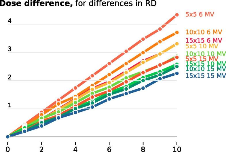
The calculated scaling factors for the different field sizes and energies to translate the differences in calculated dose.

The scaling factors offer a direct way to connect the differences in radiological depths to dose differences. They can also be used to translate the difference in radiological depths to other field sizes and energies.

References

- 1.Maier A., Syben C., Lasser T., Riess C. A gentle introduction to deep learning in medical image processing. Z Med Phys. 2019;29(2):86–101. doi: 10.1016/j.zemedi.2018.12.003. [DOI] [PubMed] [Google Scholar]
- 2.Lerner M., Medin J., Gustafsson C.J., Alkner S., Siversson C., Olsson L.E. Clinical validation of a commercially available deep learning software for synthetic CT generation for brain. Radiat Oncol. 2021;16(1):1–11. doi: 10.1186/s13014-021-01794-6. [DOI] [PMC free article] [PubMed] [Google Scholar]
- 3.Boulanger M., Nunes J.C., Chourak H., Largent A., Tahri S., Acosta O., De Crevoisier R., Lafond C., Barateau A. Deep learning methods to generate synthetic CT from MRI in radiotherapy: A literature review. Phys. Medica. 2021;89(July):265–281. doi: 10.1016/j.ejmp.2021.07.027. [DOI] [PubMed] [Google Scholar]
- 4.Maspero M., Savenije M.H.F., Dinkla A.M., Seevinck P.R., Intven M.P.W., Jurgenliemk-Schulz I.M., Kerkmeijer L.G.W., Cornelis A.T. Van Den Berg. Dose evaluation of fast synthetic-CT generation using a generative adversarial network for general pelvis MR-only radiotherapy. Phys Medi Biol. 2018;63(18):0-11. doi: 10.1088/1361-6560/aada6d. [DOI] [PubMed] [Google Scholar]
- 5.Andreasen D., Van Leemput K., Hansen R.H., Andersen J.A.L., Edmund J.M. Patch-based generation of a pseudo CT from conventional MRI sequences for MRI-only radiotherapy of the brain. Med Phys. 2015;42(4):1596–1605. doi: 10.1118/1.4914158. [DOI] [PubMed] [Google Scholar]
- 6.Klein S., Staring M., Murphy K., Viergever M.A., Pluim J.P.W. elastix: A toolbox for intensity-based medical image registration. IEEE Trans Medical Imag. 2010;29(1):196–205. doi: 10.1109/TMI.2009.2035616. [DOI] [PubMed] [Google Scholar]
- 7.Mccormick M., Liu X., Jomier J., Marion C., Ibanez L. Itk: Enabling reproducible research and open science. Front Neuroinformat. 2014;8(FEB):1–11. [Google Scholar]
- 8.Nyholm T., Svensson S., Andersson S., Jonsson J., Sohlin M., Gustafsson C., Kjellén E., Söderström K., Albertsson P., Blomqvist L., Zackrisson B., Olsson L.E., Gunnlaugsson A. MR and CT data with multiobserver delineations of organs in the pelvic area-Part of the Gold Atlas project. Med Phys. 2018;45(3):1295–1300. doi: 10.1002/mp.12748. [DOI] [PubMed] [Google Scholar]
- 9.Simko A.T., Löfstedt T., Garpebring A., Bylund M., Nyholm T., Jonsson J. vol. 143. 2021. Changing the contrast of magnetic resonance imaging signals using deep learning; pp. 713–727. (Proceedings of the Fourth Conference on Medical Imaging with Deep Learning). [Google Scholar]
- 10.Ledig C., Theis L., Huszár F., Caballero J., Cunningham A., Acosta A., Aitken A.P., Tejani A., Totz J., Wang Z., et al. Photo-realistic single image super-resolution using a generative adversarial network. Cvpr. 2017;2(3):4. [Google Scholar]
- 11.Gal Y. Dropout as a Bayesian approximation: representing model uncertainty in deep learning. ICML'16: Proceedings of the 33rd International Conference on International Conference on Machine Learning. 2016; 48: 1050–1059.
- 12.Melucci M. Relevance feedback algorithms inspired by quantum detection. IEEE Trans Knowl Data Eng. 2016;28(4):1022–1034. [Google Scholar]
- 13.Prabhat KC, Zeng R, Mehdi FM, Myers Kyle J. Deep neural networks-based denoising models for CT imaging and their efficacy. Medical Imaging 2021: Physics of Medical Imaging. 2021; February.
- 14.Dwarikanath M., Bozorgtabar B., Hewavitharanage S., Garnavi R. Medical Image Computing and Computer Assisted Intervention, (Proceedings, Part III) 2017. Image super resolution using generative adversarial networks and local saliency maps for retinal image analysis; pp. 382–391. [Google Scholar]
- 15.Jönsson, G. "Impact of MR training data on the quality of synthetic CT generation." 2022.
- 16.Zhang H., Shinomiya Y., Yoshida S. 3D Mri reconstruction based on 2D generative adversarial network super-resolution. Sensors. 2021;21(9):1–20. doi: 10.3390/s21092978. [DOI] [PMC free article] [PubMed] [Google Scholar]
- 17.Vajpayee R., Agrawal V., Krishnamurthi G. Structurally-constrained optical-flow-guided adversarial generation of synthetic CT for MR-only radiotherapy treatment planning. Sci Rep. 2022;12(1):1–10. doi: 10.1038/s41598-022-18256-y. [DOI] [PMC free article] [PubMed] [Google Scholar]
- 18.Ahnesjö A., Mania Aspradakis M. Dose calculations for external photon beams in radiotherapy. Phys Med Biol. 1999;44(11) doi: 10.1088/0031-9155/44/11/201. [DOI] [PubMed] [Google Scholar]
- 19.Nyholm T., Olofsson J., Ahnesjö A., Karlsson M. Photon pencil kernel parameterisation based on beam quality index. Radiother Oncol. 2006;78(3):347–351. doi: 10.1016/j.radonc.2006.02.002. [DOI] [PubMed] [Google Scholar]
- 20.Johnstone E., Wyatt J.J., Henry A.M., Short S.C., Sebag-Montefiore D., Murray L., Kelly C.G., McCallum H.M., Speight R. Systematic review of synthetic computed tomography generation methodologies for use in magnetic resonance imaging-only radiation therapy. Int J Radiat Oncol Biol Phys. 2018;100(1):199–217. doi: 10.1016/j.ijrobp.2017.08.043. [DOI] [PubMed] [Google Scholar]
Associated Data
This section collects any data citations, data availability statements, or supplementary materials included in this article.