Prokrustean Graph: A substring index for rapid k-mer size analysis

Abstract

Despite the widespread adoption of k-mer-based methods in bioinformatics, understanding the influence of k-mer sizes remains a persistent challenge. Selecting an optimal k-mer size or employing multiple k-mer sizes is often arbitrary, application-specific, and fraught with computational complexities. Typically, the influence of k-mer size is obscured by the outputs of complex bioinformatics tasks, such as genome analysis, comparison, assembly, alignment, and error correction. However, it is frequently overlooked that every method is built above a well-defined k-mer-based object like Jaccard Similarity, de Bruijn graphs, k-mer spectra, and Bray-Curtis Dissimilarity. Despite these objects offering a clearer perspective on the role of k-mer sizes, the dynamics of k-mer-based objects with respect to k-mer sizes remain surprisingly elusive.

This paper introduces a computational framework that generalizes the transition of k-mer-based objects across k-mer sizes, utilizing a novel substring index, the Prokrustean graph. The primary contribution of this framework is to compute quantities associated with k-mer-based objects for all k-mer sizes, where the computational complexity depends solely on the number of maximal repeats and is independent of the range of k-mer sizes. For example, counting vertices of compacted de Bruijn graphs for $k=1,\dots ,100$ can be accomplished in mere seconds with our substring index constructed on a gigabase-sized read set.

Additionally, we derive a space-efficient algorithm to extract the Prokrustean graph from the Burrows-Wheeler Transform. It becomes evident that modern substring indices, mostly based on longest common prefixes of suffix arrays, inherently face difficulties at exploring varying k-mer sizes due to their limitations at grouping co-occurring substrings.

We have implemented four applications that utilize quantities critical in modern pangenomics and metagenomics. The code for these applications and the construction algorithm is available at https://github.com/KoslickiLab/prokrustean.

1. Introduction

As the volume and number of sequencing reads and reference genomes grow every year, k-mer-based methods continue to gain popularity in computational biology. This simple approach—cutting sequences into substrings of a fixed length—offers significant benefits across various disciplines. Biologists consider k-mers as intuitive markers representing biologically significant patterns, bioinformaticians easily formulate novel methods by regarding k-mers as fundamental units that reflect their original sequences, and engineers leverage their fixed-length nature to optimize computational processes at a very low level. However, the understanding of the most crucial parameter, $k$, remains surprisingly elusive, thereby impeding further methodological advancements.

Two central challenges emerge in the application of k-mer-based methods. First, the selection of the k-mer size is often arbitrary, despite its well-recognized influence on outcomes. This issue, though widely acknowledged, remains insufficiently addressed in the literature, with little formal guidance on how to determine an optimal $k$ size for different applications. The reasoning behind these choices is frequently obscured, typically confined to specific, unpublished experimental analyses (e.g. “we found that $k=31$ was appropriate…”). Second, methods attempting to utilize multiple k-mer sizes encounter significant computational burdens. While incorporating multiple k-mer sizes can naturally enhance the accuracy of k-mer-based methods, the computational costs escalate with each additional k-mer size used. Consequently, researchers often resort to “folklore” $k$ value(s) based on prior empirical results.

The influence of k-mer sizes within each method is a complex function reflecting bioinformatics pipelines that process k-mers. As biological adjustments and engineering strategies complicate the pipelines, their outputs obscure the impact of k-mer sizes with noisy factors, as simplified in the following abstraction:

$$\text{pipeline(}k\text{-mer-based}\text{objects(}\mathit{sequences}\text{,}k\text{),}\text{biological}\text{adjustments,}\text{engineering).}$$

Despite the complexity of the pipelines, there always exist mathematically well-defined k-mer-based objects that form the foundation of method formulation. These objects abstract the utilization of k-mers and depend solely on sequences and k-mer sizes. Thus, they offer potential for generalizability and quantification of the influence of k-mers in methods. Indeed, intuitive quantities have been derived from k-mer-based objects; however, there are challenges in actually computing them, as detailed in several examples we now present.

In genome analysis, the number of distinct k-mers is often used to reflect the complexity of genomes. Although the number varies by k-mer sizes, large data sizes restrict experiments to a few $k$ values [9, 39, 15]. A recent study suggests that the number of distinct k-mers across all k-mer sizes provides additional insights into pangenome complexity [10]. Furthermore, the frequencies of k-mers provide richer information, as discussed in [1, 46], but their computation becomes more complicated and sometimes impractical, even with a fixed k-mer size [7].

In comparative analyses, Jaccard Similarity is utilized for genome indexing and searching by being approximated through hashing techniques [34, 26]. Experiments attempting to assess the influence of k-mer sizes on Jaccard Similarity must undergo tedious iterations through various k-mer sizes [8]. Additionally, Bray-Curtis dissimilarity is a k-mer frequency-based metric frequently used in comparing metagenomic samples, where experiments face resource limitations due to the growing size of sequencing data, even with a fixed k-mer size. Yet, the demand for analyzing multiple k-mer sizes continues to increase [23, 36, 35].

Genome assemblers utilizing k-mer-based de Bruijn graphs are probably the most sensitive to k-mer sizes, and those employing multi-k approaches face significant computational challenges. The choice of k-mer sizes is particularly crucial in de novo assemblers, yet it predominantly relies on heuristic methods [27, 19, 38]. The topological features of de Bruijn graphs are succinctly summarized by the compacting process, where vertices represent simple paths called unitigs, but exploring these features across varying k-mer sizes is computationally intensive. Furthermore, the development of multi-k de Bruijn graphs continues to be a challenging and largely theoretical endeavor [40, 43, 22], with no substantial advancements following the heuristic selection of multiple k-mer sizes implemented by metaSPAdes [33].

These examples motivate the pressing need to generalize the exploration of k-mer-based objects across k-mer sizes. Our manuscript introduces a framework for rapidly computing quantities derived from k-mer-based objects, thereby addressing the prevalent challenge in bioinformatics. The organization of the manuscript is as follows:

• Section 2 defines the main objective of computing k-mer-based quantities and introduces the proxy problem of computing substring co-occurrence.

• Section 3 defines ${𝒢}_{𝒰}$, the Prokrustean graph, a novel substring representation that provides straightforward access to substring co-occurrence.

• Section 4 outlines a framework built upon the Prokrustean graph, accompanied by algorithms that treat various k-mer-based objects and compute related quantities across all possible k-mer sizes in $O\left(\right|{𝒢}_{𝒰}\left|\right)$ time.

• Section 5 presents the experimental results of computing k-mer-based quantities.

• Section 6 derives the construction algorithm of ${𝒢}_{𝒰}$, and discusses the limitations of other modern substring indices in computing substring co-occurrence.

2. Problem Formulation

2.1. Basic Notations

Let $\mathrm{\Sigma }$ be our alphabet and let $S\in \mathrm{\Sigma }\mathrm{*}$ represent a finite-length string, and $𝒰\subset \mathrm{\Sigma }\mathrm{*}$ for a set of strings. Because of the biological sequence motivation for this work, the elements of $𝒰$ are called sequences. Consider the following preliminary definitions:

Definition 1.

• A region in the string $S$ is a triple ($S,i,j$) such that $1\le i\le j\le \left|S\right|$.

• The string of a region is the corresponding substring: $str\left(S,i,j\right):=S_i{S}_{i+1}\dots S_j$.

• The size or length of a region is the length of its string: $\left|S,i,j\right|:=j-i+1$.

• An extension of a region $(S,i,j)$ is a larger region $\left(S,i^{\prime },j^{\prime }\right)$ including $(S,i,j)$:

  $$(S,i,j)⊊\left(S,i^{\prime },j^{\prime }\right):=i^{\prime }\le i\le j\le j^{\prime }\text{and}\left|\right(S,i,j\left)\right|<\left|\left(S,i^{\prime },j^{\prime }\right)\right|\text{.}$$
• The occurrences of $S$ in $𝒰$ are those regions in strings of $𝒰$ corresponding to $S$:

  $${occ}_{𝒰}\left(S\right):=\left\{\left(S^{\prime },i,j\right)\mid S^{\prime }\in 𝒰\&str\left(S^{\prime },i,j\right)=S\right\}.$$

• $S$ is a maximal repeat in $𝒰$ if it occurs at least twice and more than any of its extensions: $\left|{occ}_{𝒰}\left(S\right)\right|>1$, and for all $S^{\prime }$ a superstring of $S$, $\left|{occ}_{𝒰}\right(S\left)\right|>\left|{occ}_{𝒰}\left(S^{\prime }\right)\right|$. I.e., given a fixed set $𝒰$, a maximal repeat $S$ is one that occurs more than once in $𝒰$ (i.e. is a repeat), and any extension of which has a lower frequency in $𝒰$ than the original string $S$.

• ${ℛ}_{𝒰}$ is the set of all maximal repeats in $𝒰$.

2.2. The proxy problem: how to compute substring co-occurrence?

There exists a theoretical void in identifying when a k-mer and a $k^{\prime }$-mer serve similar roles within their respective substring sets. Although close k-mer sizes generally yield comparable outputs, dissecting this phenomenon at the level of local substring scopes is unexpectedly challenging. For instance, de Bruijn graphs constructed from sequencing reads with $k=30$ and $k^{\prime }=31$ display distinct yet highly similar topologies [40]. However, anyone formally articulating the topological similarity would find it quite elusive, as vertex mapping and other techniques establishing correspondences between the two graphs fail to consistently explain it.

A common underlying difficulty is that the entire k-mer set undergoes complete transformations as the k-mer size changes. Since the role of a k-mer is assigned within its k-mer set, the role of a $k^{\prime }$-mer within $k^{\prime }$-mers cannot be “locally” derived. To address this issue, we propose substring co-occurrence as a generalized framework for consistently grouping k-mers of similar roles across varying k-mer sizes.

Definition 2.

A string $S$ co-occurs within a string $S^{\prime }$ in $𝒰$ if:

$$S\mathit{is}\mathit{a}\mathit{substring}\mathit{of}{S}^{\prime }\mathit{and}\left|oc{c}_{𝒰}\left(S\right)\right|=\left|oc{c}_{𝒰}\left(S^{\prime }\right)\right|.$$

Modern substring indexes built on longest common prefixes (LCP) of their (implicit) suffix array are adept at capturing co-occurrence in this “extending direction.” In suffix trees, a substring that extends from $S$ to $S^{\prime }$ along an edge—without passing through a node—indicates preservation of co-occurrence. Similarly, in the Burrows-Wheeler Transform (BWT) and its variants such as the FM-index and r-index, representing both $S$ and $S^{\prime }$ with the same set of LCPs corresponding to some suffix array interval implies co-occurrence. However, there has been no recognized necessity for addressing the following “substring direction”:

Definition 3.

${co-substr}_{𝒰}\left(S\right)$ is the set of substrings that co-occur within $S$.

Modern substring indexes are not efficient at computing ${co-substr}_{𝒰}\left(S\right)$, which results in their failure to “smoothly” explore k-mer-based objects across varying k-mer sizes. Specifically, shrinking a substring found in $𝒰$ always requires some link (or pointer) to navigate to the corresponding LCP in the (implicit) suffix array. Given that the number of substrings scales quadratically with the cumulative size of the input sequences, this linkage system becomes impractical. For instance, the variable-order de Bruijn graph and its variants address the space issue by employing a compact de Bruijn graph representation built above the Burrow-Wheeler transform [12]; however, this solution requires nontrivial operation times for both “forward” moves and changes in order ($k$) [11, 5]. So, these data structures do not allow extensive exploration of the substring space, and hence their multi-k approaches do not scale well.

Our work demonstrates that ${co-substr}_{𝒰}\left(S\right)$ can be computed efficiently, and then the functionality can be used to rapidly compute k-mer quantities. We introduce a simple yet foundational property as groundwork.

Theorem 1 (Principle).

For any substring $S$ such that $o{cc}_{𝒰}\left(S\right)>0$,

$$S\mathit{co}-\mathit{occurs}\mathit{within}\mathit{exactly}\mathit{one}\mathit{sequence}\mathit{or}\mathit{maximal}\mathit{repeat}\mathit{in}𝒰\cup {ℛ}_{𝒰}$$

Proof. Assume the theorem does not hold, i.e., $S$ co-occurs within either no string or multiple strings in $𝒰\cup {ℛ}_{𝒰}$. Consider the former case: $S$ co-occurs within no string in $𝒰\cup {ℛ}_{𝒰}$, meaning $S$ occurs more than any of its superstrings in $𝒰\cup {ℛ}_{𝒰}$. Given that $S$ occurs in some string $S^{\prime }\in 𝒰$ $(i.e.o{cc}_{𝒰}(S)>0)$, $S$ must be occurring more frequently than $S^{\prime }$ by assumption. Then, there exists a maximal repeat $R$ such that $S$ is a substring of $R$ and $R$ is a substring of $S^{\prime }$, because extending $S$ within $S^{\prime }$ decreases its occurrence at some point. Again, whenever $S$ is a substring of a maximal repeat $R$, $S$ must be occurring more frequently than $R$ by assumption. Following the similar argument above, there exists another maximal repeat $R^{\prime }$ such that $S$ is a substring of $R^{\prime }$ and $R^{\prime }$ is a proper substring of $R$. This recursive argument will eventually terminate as $R^{\prime }$ is strictly shorter than $R$. Thus, $S$ co-occurs within the last maximal repeat, which contradicts the assumption.

Now consider the latter case where $S$ co-occurs within at least two strings in $𝒰\cup {ℛ}_{𝒰}$. If $S$ is extended within these two strings, either to the right or left by one step at each time, the extensions eventually diverge into two different strings since the two superstrings differ, thereby reducing the number of occurrences. Hence, $S$ must be occurring more frequently than at least one of those two superstrings, leading to a contradiction. □

This theorem provides two key insights. First, every substring found in $𝒰$ exclusively co-occurs as a substring of either a sequence or a maximal repeat in $𝒰$, so the collective sets of $co-subst{r}_{𝒰}\left(S\right)$ from every $S\in 𝒰\cup {ℛ}_{𝒰}$ comprehensively and disjointly cover the entire substring space. Second, by computing $co-subst{r}_{𝒰}\left(S\right)$ for every $S\in 𝒰\cup {ℛ}_{𝒰}$, we can categorize k-mers of similar roles across various lengths, devising various algorithmic ideas on $co-subst{r}_{𝒰}\left(S\right)$. The following main theorem outlines the components discussed in the remainder of the manuscript.

Theorem 2. (Main Result)

Given a set of sequences $𝒰$, there exists a substring representation ${𝒢}_{𝒰}$ of size $O\left(\left|\mathrm{\Sigma }\right|\cdot \left|{ℛ}_{𝒰}\right|\right)$. ${𝒢}_{𝒰}$ can be used to compute k-mer quantities of $𝒰$ for all $k=1,\dots ,k_{\mathrm{m}\mathrm{a}\mathrm{x}}$ within $O\left(\right|{𝒢}_{𝒰}\left|\right)$ time and space, where $k_{\mathrm{m}\mathrm{a}\mathrm{x}}$ is the longest sequence length in $𝒰$. The k-mer quantities are given as follows:

• (Counts) The number of distinct k-mers, as used in genome cardinality DandD [10].

• (Frequencies) k-mer Bray-Curtis dissimilarities, as used in comparing metagenomic samples [36].

• (Extensions) The number of unitigs in k-mer de Bruijn graphs, as used in analyses of reference genomes and genome assembly [29, 42].

• (Occurrences) The number of edges with annotated length of $k$ in the overlap graph. [45].

Furthermore, the graph ${𝒢}_{𝒰}$ can be constructed in $O\left(\right|BWT|+|{𝒢}_{𝒰}\left|\right)$ time and space, where $\left|BWT\right|$ is the size of the Burrows-Wheeler transform representation of $𝒰$.

Proof. Section 3 analyzes the size of ${𝒢}_{𝒰}$, Section 4 introduces the computation of k-mer quantities, and Section 6 derives the construction algorithm. □

The main contribution is that the time complexity for computing k-mer quantities for all $k\in \left[1,k_{\mathrm{m}\mathrm{a}\mathrm{x}}\right]$ using ${𝒢}_{𝒰}$ is independent of the range of k-mer sizes, which is $O\left(\left|{𝒢}_{𝒰}\right|\right)$. Specifically, letting $N$ be the cumulative sequence length of $𝒰$, $\left|{𝒢}_{𝒰}\right|$ is sublinear relative to $N$. In contrast, the direct computation of k-mer quantities from the sequence set $𝒰$ for any fixed k-mer size demands, at best, $O\left(N\right)$ time. Extending this computation naively to cover all $k=1,\dots ,k_{\mathrm{m}\mathrm{a}\mathrm{x}}$ would exponentially increase the computational demand to $O(N^{k_{\mathrm{m}\mathrm{a}\mathrm{x}}})$. This significant improvement in complexity leverages a proper representation of repeats in $𝒰$, as will be introduced in the next section.

3. Prokrustean graph: A hierarchy of maximal repeats

The key idea of the Prokrustean graph is to recursively capture maximal repeats by their relative frequencies of occurrences in $𝒰$. Consider the following two descriptions of repeats in three sequences: ACCCT, GACCC, and TCCCG.

1. ACCC is in 2 sequences, and CCC is in all 3 sequences.

2. ACCC is in 2 sequences, and CCC is in 1 sequence TCCCG and 1 substring ACCC.

Each first and second case uses 5 and 4 units of occurrences, respectively, yet preserves the same meaning. As depicted in Figure 1, the rule of the compact second case is to recursively capture regions of more frequent substrings.

Figure 1:

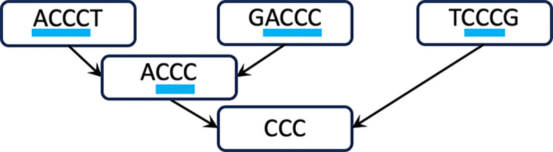
Recursive repeats. At each sequence on the top level, maximally long subregions (indicated with blue underlining) are used to denote substrings that are more frequent than its superstring. The arrows then points to a node of the substring, and the process repeats hierarchically.

Definition 4.

$(S,i,j)$ is a locally-maximal repeat region in $𝒰$ if:

$$\left|{occ}_{𝒰}\left(str\right(S,i,j\left)\right)\right|>\left|oc{c}_{𝒰}\left(S\right)\right|$$ (1)

and for each extension $\left(S,i^{\prime },j^{\prime }\right)$ of $(S,i,j)$,

$$\left|oc{c}_{𝒰}\left(str\left(S,i^{\prime },j^{\prime }\right)\right)\right|=\left|{occ}_{𝒰}\left(S\right)\right|.$$ (2)

**Note that we often omit “in $𝒰$” when the context is clear.

A locally-maximal repeat region captures a substring that appears more frequently than the “parent” string, and any extension of the region captures a substring that appears as frequently as the parent string. Consider the previous example $𝒰=\{\mathrm{A}\mathrm{C}\mathrm{C}\mathrm{C}\mathrm{T},\mathrm{G}\mathrm{A}\mathrm{C}\mathrm{C}\mathrm{C},\mathrm{T}\mathrm{C}\mathrm{C}\mathrm{C}\mathrm{G}\}$. (ACCCT,1,4) is a locally-maximal repeat region capturing the substring ACCC in ACCCT. However, (ACCCT,2,4) is not a locally-maximal repeat region because the region capturing CCC in ACCCT can be extended to the left to capture ACCC which occurs more frequently than ACCCT.

Note, an alternative definition using substring notations, such as locally-maximal repeats, instead of regions, is not robust. Consider $𝒰=\{\mathrm{A}\mathrm{C}\mathrm{C}\mathrm{C}\mathrm{T}\mathrm{C}\mathrm{C}\mathrm{G},\mathrm{G}\mathrm{C}\mathrm{C}\mathrm{C}\}$ and $S:=\mathrm{A}\mathrm{C}\mathrm{C}\mathrm{C}\mathrm{T}\mathrm{C}\mathrm{C}\mathrm{G}$. Observe that the region $(S,2,4)$ capturing CCC is a locally-maximal repeat region because CCC occurs more frequently than $S$ in $𝒰$, but its immediate left and right extensions capture ACCC and CCCT that occur the same number of times as $S$. In constrast, a subregion $(S,2,3)$ capturing CC is not a locally-maximal repeat region because an extension $(S,2,4)$ still captures a string (CCC) which occurs 2 times in $𝒰$ which is more than $S$. However, $(S,6,7)$, which also captures CC, is a locally-maximal repeat region because $\left|o{cc}_{𝒰}\left(\mathrm{C}\mathrm{C}\right)\right|=5>\left|o{cc}_{𝒰}\left(S\right)\right|=1$ and $\left|o{cc}_{𝒰}\left(S\right)\right|=\left|o{cc}_{𝒰}\left(\mathrm{T}\mathrm{C}\mathrm{C}\right)\right|=\left|o{cc}_{𝒰}\left(\mathrm{C}\mathrm{C}\mathrm{G}\right)\right|$. Consequently, defining a locally-maximal repeat as $S_{6..7}=\mathrm{C}\mathrm{C}$ becomes ambiguous with $S_{2..3}=\mathrm{C}\mathrm{C}$, whereas an explicit expression of a region $(S,6,7)$ more accurately reflects the desired property of hierarchy of occurrences.

3.1. Prokrustean Graph

The Prokrustean graph of $𝒰$ is simply a graph representation of recursive locally-maximal repeat regions on $𝒰$, i.e. vertexes represent substrings and edges represent locally-maximal repeat regions. The theorem below says that all maximal repeats in $𝒰$ are caught along the recursive description.

Theorem 3 (Complete).

Construct a string set $\mathbf{R}\left(𝒰\right)$ as follows:

1. for each locally-maximal repeat region $(S,i,j)$ where $S\in 𝒰$, add $str(S,i,j)$ to $\mathbf{R}\left(𝒰\right)$ and

2. for each locally-maximal repeat region $(S,i,j)$ where $S\in \mathbf{R}\left(𝒰\right)$, add $str(S,i,j)$ to $\mathbf{R}\left(𝒰\right)$.

   $$Itfollowsthat\mathbf{R}\left(𝒰\right)={ℛ}_{𝒰}holds.$$

Proof. Any string in $\mathbf{R}\left(𝒰\right)$ is a maximal repeat of $𝒰$, so the claim is satisfied if the process captures every maximal repeat of $𝒰$. Assume a maximal repeat $R$ is not in $\mathbf{R}\left(𝒰\right)$. Consider any occurrence of $R$ in some $S\in 𝒰$. Extending the maximal repeat $R$ within $S$ makes the number of its occurrences drop, but since $R$ cannot occur as a locally-maximal repeat region by assumption, it must be included in some locally-maximal repeat region that captures a maximal repeat $R_1$, hence $R_1\in \mathbf{R}\left(𝒰\right)$, and $R$ is a proper substring of $R_1$. Now consider any occurrence of $R$ within $R_1$. This argument continues recursively, capturing maximal repeats $R_1,R_2,\dots$, but cannot extend indefinitely as $R_{i+1}$ is always shorter than $R_i$ for every $i\ge 1$. Eventually, $R$ must be occurring as a locally-maximal repeat region of some $R_n$, which is a contradiction. □

Therefore, we use maximal repeats as vertices of the Prokrustean graph, along with sequences, so $𝒰\cup {ℛ}_{𝒰}$.

Definition 5.

The Prokrustean graph of $𝒰$ is a directed multigraph ${𝒢}_{𝒰}:=\left({𝒱}_{𝒰},{ℰ}_{𝒰}\right)$:

• ${𝒱}_{𝒰}:v_S\in {𝒱}_{𝒰}$ if and only if $S\in 𝒰\cup {ℛ}_{𝒰}$.

• Each vertex $v_S\in {𝒱}_{𝒰}$ is annotated with the string size, $size\left(v_S\right)=\left|S\right|$.

• ${ℰ}_{𝒰}:e_{S,i,j}\in {ℰ}_{𝒰}$ if and only if $(S,i,j)$ is a locally-maximal repeat region.

• Each edge $e_{S,i,j}\in {ℰ}_{𝒰}$ directs from $v_{S}to{v}_{str(S,i,j)}$ and is annotated with interval $\left(e_{S,i,j}\right):=(i,j)$, to represent the locally-maximal repeat region.

Figure 2 visualizes how locally-maximal repeat regions are encoded in a Prokrustean graph. Next, the cardinality analysis of this representation reveals promising bounds.

Figure 2:

The Prokrustean graph of $𝒰=\{\mathrm{A}\mathrm{C}\mathrm{C}\mathrm{C}\mathrm{T},\mathrm{G}\mathrm{A}\mathrm{C}\mathrm{C}\mathrm{C},\mathrm{T}\mathrm{C}\mathrm{C}\mathrm{C}\mathrm{G},\mathrm{G}\mathrm{G}\mathrm{C}\mathrm{G}\}$. The left graph describes the recursion of locally-maximal repeat regions, and the Prokrustean graph on the right represents the same structure with integer labels storing the regions and the size of the substrings.

Theorem 4 (Compact). $\left|{ℰ}_{𝒰}\right|\le 2\left|\mathrm{\Sigma }\right|\left|{𝒱}_{𝒰}\right|$

Proof. Every vertex in ${𝒱}_{𝒰}$ has at most one incoming edge per letter extension on the right (or similarly on the left), so has at most $2\left|\mathrm{\Sigma }\right|$ incoming edges. Assume the contrary: a maximal repeat appears as two different locally-maximal repeat regions $(S,i,j)$ and $\left(S^{\prime },i^{\prime },j^{\prime }\right)$ within $S,S^{\prime }\in 𝒰\cup {ℛ}_{𝒰}$, and can extend by the same letter on the right, i.e., $(S,i,j+1)$ and $\left(S^{\prime },i^{\prime },j^{\prime }+1\right)$ capture the same string. Extending these regions further together will eventually diverge their strings, because either $S\ne S^{\prime }$ or the original two regions are differently located even if $S=S^{\prime }$. Consequently, at least one of them—$(S,i,j+1)$ without loss of generality—results in a decreased occurrence count of its string as it extends. Hence, $\left|o{cc}_{𝒰}\left(str\right(S,i,j+1\left)\right)\right|>\left|o{cc}_{𝒰}\left(S\right)\right|$. This leads to contradiction because a locally-maximal repeat region $(S,i,j)$ should satisfy $\left|oc{c}_{𝒰}(S,i,j+1)\right|=\left|oc{c}_{𝒰}(S,1,|S\left|\right)\right|$. □

Assuming trivially that $\left|𝒰\right|\ll \left|{ℛ}_{𝒰}\right|$, meaning there are significantly more maximal repeats than the number of sequences, we derive that $O\left(\left|{𝒱}_{𝒰}\right|\right)=O\left(\left|{ℛ}_{𝒰}\right|\right)$, hence $O\left(\left|{𝒢}_{𝒰}\right|\right):=O\left(\left|{ℰ}_{𝒰}\right|\right)=O\left(\left|\mathrm{\Sigma }\right|\left|{ℛ}_{𝒰}\right|\right)$ by the theorem. Given that $\left|\mathrm{\Sigma }\right|$ is typically constant in genomic sequences (eg. $\mathrm{\Sigma }=\{A,C,T,G\}$), the graph’s size depends on the number of maximal repeats. Letting $N$ be the accumulated sequence length of $𝒰$, it is a well-known fact that $\left|{ℛ}_{𝒰}\right|<N$ [25], so the graph grows sublinear to the input size. Furthermore, in the implementations described in Section 5, ${ℛ}_{𝒰}$ can be restricted to maximal repeats of length at least $k_{\mathrm{m}\mathrm{i}\mathrm{n}}$. Although the size of ${𝒢}_{𝒰}$ is comparable to that of the suffix tree of $𝒰$, setting $k_{\mathrm{m}\mathrm{i}\mathrm{n}}$ allows for significantly more efficient and configurable space usage.

4. Framework: Computing k-mer quantities for all $\mathit{k}$ sizes

This section introduces the computation of k-mer quantities for all $k$ sizes, preserving the $O\left(\right|{𝒢}_{𝒰}\left|\right)$ time and space.

4.1. Accessing co-occurring k-mers for a single $k$ size

We briefly cover how k-mers of a fixed k-mer size are accessed through the Prokrustean graph, before generalizing the computation to all k-mer sizes in the next section. Previously, a toy example in Figure 1 depicted blue regions that cover locally-maximal repeat regions. Then, given a k-mer size, a complementary region is a maximal region that covers k-mers that are not included in a blue region. See the red regions underlining in Figure 3.

Figure 3:

Accessing k-mers by complementing locally-maximal repeat regions. Blue underlining depicts locally-maximal regions, and red underlining depicts regions that complemented k-mers not covered in blue regions, given sizes of $k=3$ and 4. Every k-mer appears exactly once within a red region. For example, at the figure of $k=3$ on left, the 3-mer ACC is included in a red region in ACCCC and does not appear again in any other red region.

An opportunistic property is that k-mers in red regions co-occur within their parent strings. Following notation captures substrings in red regions:

Defin ition 6.

A string $S$ k-co-occurs within a string $S^{\prime }$ in $𝒰$ if:

$$everyk-merinSco-occurswithin{S}^{\prime }in𝒰.$$

We mean the same by $S$ being a k-co-occuring substring of $S^{\prime }$. Also, $S$ maximally k-co-occurs within $S^{\prime }$ in $𝒰$ if no superstring of $S$ k-co-occurs within $S^{\prime }$ in $𝒰$. Maximal k-co-occurring substrings of $S^{\prime }$ are easily computed as complementary regions in $S^{\prime }$ as introduced in Figure 3. So, they are efficiently identified with the Prokrustean graph, as implied by the proposition below.

Proposition 1.

A string $S$ maximally k-co-occurs within a string $S^{\prime }$ in $U$ if and only if its region in $S^{\prime }$ intersect locally-maximal repeat regions by under $k-1$, and on both sides, either extends to an end of $S^{\prime }$ or intersects a locally-maximal repeat region by exactly $k-1$.

Proof. The forward direction is straightforward: if $S$ k-co-occurs within $S^{\prime }$, its region cannot intersect any locally-maximal repeat region by $k$ at any case, and if the intersection is under $k-1$ on its edge, by extending $S$ and making the intersection $k-1$, another superstring of $S$ k-co-occurs within $S^{\prime }$.

For the reverse direction, assume a region satisfies the conditions. A k-mer appearing in the region cannot occur more than $S$, as it would mean the region intersects a locally-maximal repeat region by at least $k$, so $S^{\prime }$ k-co-occurs within $S$. $S^{\prime }$ is also maximal because extending its region increases the size of the intersection to more than $k-1$. □

Proposition 1 implies that computing maximal k-co-occurring substrings of a string $S$ takes time linear to the number of locally-maximal repeat regions in $S$, given the regions pre-ordered by positions: Enumerate locally-maximal repeat regions of length at least $k$ and check its left and right whether a complementary region of length at least $k$ can be defined. Lastly, maximally capture complementary regions on both sides so that they either intersect locally-maximal repeat regions by $k-1$ or meet an end of $S$. See Figure 4 for a detailed example.

Figure 4:

Computing k-co-occurring substrings (red) of $S$ of varying $k$ sizes. The rule is to cover every k-mer that is not covered by a locally-maximal repeat region (blue). Note that a k-co-occurring substring can appear on the intersection of two locally-maximal repeat regions too. For example, the region ($S,3,6$) capturing CAGC in the second row ($k=4$) overlaps two blue regions by 3.

Therefore, the idea for computing complementary regions can be applied to count distinct k-mers for a fixed k-mer size. The toy algorithm below takes $O\left(\right|{𝒢}_{𝒰}\left|\right)$ time and space.

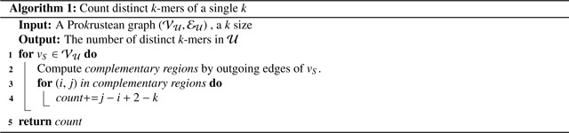
Note that line 2 is the computation derived from Proposition 1, as depicted in Figure 4. The locally-maximal repeat regions of $S$ are represented by the outgoing edges of $v_S$. The nested loop on lines 1 and 2 thus takes $O\left(\left|{ℰ}_{𝒰}\right|\right)$, i.e., $\left.O\left(\left|\mathrm{\Sigma }\right|\left|{ℛ}_{𝒰}\right|\right)\right)$ time. For correctness, Theorem 1 states that any k-mer $K$ co-occurs within exactly one string $S$ in $𝒰\cup {ℛ}_{𝒰}$. $K$ extends to a unique maximal k-co-occurring substring of $S$; otherwise, multi-occurrence in $S$ is implied. Lastly, Proposition 1 guarantees that every maximal k-co-occurring substring of $S$ can be identified by scanning the outgoing edges of $v_S$.

4.2. Accessing co-occurring k-mers for a range of $k$

The computation can be extended to a range of k-mer sizes while preserving the complexity. Recall that the problem is to efficiently express ${co-substr}_{𝒰}\left(S\right)$. It turns out that ${co-substr}_{𝒰}\left(S\right)$ can be expressed by a finite number of stack-like substring structures.

Definition 7.

Consider two strings $S$ and $T$ where $T$ is a substring of $S$, along with two numbers: a depth $d\mathrm{*}$ and a k-mer size $k\mathrm{*}$, each at least 1. A co-occurrence stack of $S$ in $U$ is defined as a 4-tuple:

$$(S,T,k^{\mathrm{*}},d^{\mathrm{*}})$$

$$\mathit{when}str\left(T,1+{\delta }_l\cdot (i-1),\left|T\right|-{\delta }_r\cdot (i-1)\right)\mathit{maximally}{k}_i\mathit{-co-occurs}\mathit{within}S$$

where $k_i=k^{\mathrm{*}}-\left(i-1\right)$ for $i=1,2,\dots ,d^{\mathrm{*}}$, with change rates ${\delta }_l:=1_{TisNOTaprefixofS}$ and ${\delta }_r:=1_{TisNOTasuffixofS}$ .

A co-occurrence stack expresses a k-mer if it is a substring of some k-co-occurring substring identified by the stack. A co-occurrence stack is maximal if its expressed k-mers are not a subset of those expressed by any other co-occurrence stack. It is clear that any k-mer expressed in a co-occurrence stack of $S$ co-occurs within $S$. So, maximal co-occurrence stacks of $S$ collectively express ${co-substr}_{𝒰}\left(S\right)$.

Definition 8.

${co-stack}_{𝒰}\left(S\right)$ is the set of all maximal co-occurrence stacks of $S$ in $𝒰$.

A maximal co-occurrence stack of $S$ is type-0 if the substring $T$ is $S$ itself, type-1 if $T$ is a proper prefix or suffix of $S$, and type-2 otherwise. The numeral in each type’s name indicates the number of locally-maximal repeat regions intersecting the regions of substrings identified by the co-occurrence stack. Refer to Figure 5 for intuition on the type names.

Figure 5:

Three types of maximal co-occurrence stacks of $S$ (sets of red rectangles), given two locally-maximal repeat regions in $S$ (blue rectangles). The Rate column describes the change in the count of expressed k-mers as the k-mer size increases by 1. Hence, the rate is $1-{\delta }_l-{\delta }_r$, and it controls the vertical shapes of stacks.

Theorem 5.

${co-stack}_{𝒰}\left(S\right)$ completely and disjointly cover co-occurring substrings of $S$, i.e.,

$${co-substr}_{𝒰}(S)=\underset{(S,T,k^{\mathrm{*}},d^{\mathrm{*}})\in {co-stack}_{𝒰}(S)}{⨆}\{\mathit{substrings}\mathit{expressed}\mathit{by}(S,T,k^{\mathrm{*}},d^{\mathrm{*}})\}.$$

Also,

$$\mid {\mathit{co-stack}}_{𝒰}(S)\mid \le 1+2\cdot (\mathit{the}\mathit{number}\mathit{of}\mathit{locally-maximal}\mathit{repeat}\mathit{regions}\mathit{in}S)$$

Proof. Appendix B.1 covers the proof. □

Lastly, this scheme is extended to the entire substring space. Also, all maximal co-occurrence stacks in $𝒰$ can be enumerated within the computation time $O\left(\left|{ℰ}_{𝒰}\right|\right)$.

Proposition 2.

The number of all maximal co-occurrence stacks in $𝒰$ is $O\left(|{𝒢}_{𝒰}\right)|$. Precisely,

$$\sum _{S\in 𝒰\cup {ℛ}_{𝒰}}|{\mathit{co-stack}}_{𝒰}(S)|\le \left|{𝒱}_{𝒰}\right|+2\left|{ℰ}_{𝒰}\right|.$$

Proof. This is implied by the inequality ${|co-stack}_{𝒰}(S)|\le 1+2$(the number of locally-maximal repeat regions in $S$). The term $\left|{𝒱}_{𝒰}\right|$ accounts for the constant contribution of 1 from each $S\in 𝒰\cup {ℛ}_{𝒰}$, and $2\left|{ℰ}_{𝒰}\right|$ corresponds to the right term because ${ℰ}_{𝒰}$ represents the total set of locally-maximal repeat regions in $𝒰\cup {ℛ}_{𝒰}$. □

Proposition 3.

Given ${𝒢}_{𝒰}$, enumerating $co-{stack}_{𝒰}(S)$ for some $v_S\in {𝒱}_{𝒰}$ takes $O(|outgoingedgesof\left.v_S\mid \right)$ time.

Proof. This is derived from the proof of $\left|co-{stack}_{𝒰}(S)\right|\le 1+2\cdot$ the number of locally-maximal repeat regions in $S$ in Appendix B.1. □

Since k-mers expressed by each stack of $S$ inherit characteristics of $S$, such as frequency and extensions within $𝒰$, algorithms can leverage this information to compute k-mer quantities, by considering k-mers in the same stack as having similar roles in the k-mer-based objects. We further introduce four applications motivated by biological problems that benefit from this methodology.

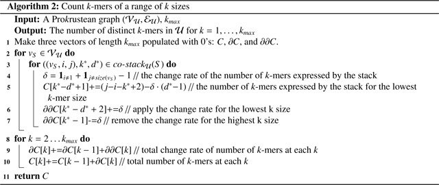
4.3. Application: Counting distinct k-mers of all $k$ sizes

The number of distinct k-mers is commonly used to assess the complexity and structure of pangenomes and metagenomes [44, 13]. A recent study by [10] spans multiple $k$ contexts, suggesting that the number of k-mers across all k-mer sizes should be used to estimate genome sizes. The following algorithm counts distinct k-mers for all k-mer sizes in time $O\left(\left|{𝒢}_{𝒰}\right|\right)$. We assume the maximum possible k-mer size, $k_{max}$, is always less than $\left|{ℰ}_{𝒰}\right|$, which is typical for most sequencing data and genome references.

The core idea leverages the change rate of k-mers within each co-occurrence stack, thereby eliminating the need to consider k-mer counts individually. The number of k-mers expressed by each type-0, 1, or 2 co-occurrence stack changes by −1, 0, or +1 as $k$ increases by 1, respectively, as detailed in the Rate column of Figure 5. This property is utilized in lines 4–7, and hence the loop in line 2 runs in $O\left(\left|{𝒢}_{𝒰}\right|\right)$ time.

4.4. Application: Computing Bray-Curtis dissimilarities of all $k$ sizes

The Bray-Curtis dissimilarity, defined with k-mers, is a frequency-based metric that measures the dissimilarity between biological samples. The values are sensitive to the choice of k-mer sizes, so they are often calculated with multiple k-mer sizes to check the influence [47] [23] [36], yet most state-of-the-art tools utilize a fixed k-mer size [7].

We computed the Bray-Curtis dissimilarity for all k-mer sizes of samples A and B using the Prokrustean graph constructed from the union of their sequence sets, ${𝒰}_A$ and ${𝒰}_B$. This graph tracks the origins of sequences, computing the following quantities:

$$BC\left({𝒰}_A,{𝒰}_B,k\right)=1-\frac{k\text{-mer}\text{in}{𝒰}_A\cup {𝒰}_{B}2\cdot \mathrm{m}\mathrm{i}\mathrm{n}\left({\mathrm{f}\mathrm{r}\mathrm{e}\mathrm{q}}_A(k\text{-mer}),{\mathrm{f}\mathrm{r}\mathrm{e}\mathrm{q}}_B(k\text{-mer})\right)}{k\text{-mer}\text{in}{𝒰}_A\cup {𝒰}_B{\text{freq}}_A(k\text{-mer})+{\mathrm{f}\mathrm{r}\mathrm{e}\mathrm{q}}_B(k\text{-mer})}$$

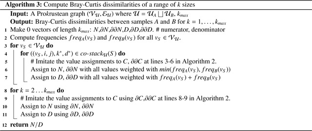
Recall that the value assignments in line 5 and 6 utilized co-occurrence stacks for counting k-mers in Algorithm 2. The values $\mathrm{m}\mathrm{i}\mathrm{n}\left(fre{q}_A\left(v_S\right),fre{q}_B\left(v_S\right)\right)$ and $fre{q}_A\left(v_S\right)+fre{q}_B\left(v_S\right)$ are assigned instead of a constant 1, because they grows linear to the number of co-occurring k-mers weighted by the frequency-based values. Consequently, vectors $N$ and $D$ contains values of the numerator and denominator part of the Bray-Curtis dissimilarities for all k-mer sizes.

Typically, biological experiments compute these values for pairs of multiple samples. The proposed algorithm can be extended to consider multiple samples, requiring $O({\left|\mathrm{s}\mathrm{a}\mathrm{m}\mathrm{p}\mathrm{l}\mathrm{e}\mathrm{s}\right|}^2\mathrm{·}|{𝒢}_{𝒰}|)$ time.

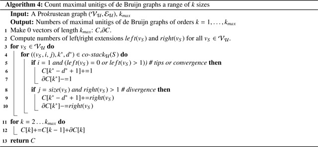
4.5. Application: Counting maximal unitigs of all $k$ sizes

A maximal unitig of a de Bruijn graph, or a vertex of a compacted de Bruijn graph [20], represents a simple path that cannot be extended further, reflecting a topological characteristic of the graph. More maximal unitigs generally indicate more complex graph structures, which significantly impact genome assembly performance [14, 3]. Their number across multiple k-mer sizes reflects the influence of k-mer sizes on the complexity of assembly.

The idea is that maximal unitigs are implied by tips, convergences, and divergences, which are indicated by type-0 or 1 co-occurrence stacks. For instance, consider a string $S$ in $𝒰\cup {ℛ}_{𝒰}$ with multiple right extensions, such as C and T. If a suffix region in $S$ of length $l$ is an locally-maximal repeat region, it suggests that a k-co-occurring suffix of $S$ where $k>l$ corresponds to a vertex in the respective de Bruijn graph of order $k$ with right extensions C and T. Therefore, identifying the locally-maximal repeat regions on suffixes and prefixes of strings in $𝒰\cup {ℛ}_{𝒰}$ is sufficient.

4.6. Application: Computing vertex degrees of overlap graph

Overlap graphs are extensively utilized in genome and metagenome assembly, alongside de Bruijn graphs. Although their definition appears unrelated to k-mers, we can view them as representing suffix-prefix k-mers of sequences in $𝒰$. Overlap information is particularly crucial for metagenomics in read classification [16, 41, 31, 2] and contig binning [45, 32]. Vertex degrees are often interpreted as (abundant-weighted) read coverage in metagenomic samples, which exhibit high variances due to species diversity and abundance variability.

A common computational challenge is the quadratic growth of overlap graphs relative to the number of reads $O(|𝒰{|}^2)$. A significant drawback of overlap graphs is their quadratic growth in the number of reads, $O(|𝒰{|}^2)$. In contrast, the Prokrustean graph, which encompasses the overlap graph as a hierarchical subgraph, requires only $O(|{𝒢}_{𝒰}|)$ space. This structure enables the efficient computation of vertex degrees in the overlap graph.

The overlap graph of $𝒰$ has the vertex set $𝒰$, and an edge ($v_S,v_{S^{\prime }}$) if and only if a suffix of $S$ matches a prefix of $S^{\prime }$. Define $pref\left(v_R\in {𝒱}_{𝒰}\right)$ as the number of $R$ occurring as a prefix in strings in $𝒰$, which is easily computed through the recursive structure.

$$pref\left(v_R\in {𝒱}_{𝒰}\right):=\sum _{e=\left(v_{R^{\prime }},v_{ℛ}\right)\in {ℰ}_{𝒰},\mathit{region}(e)=(1,\mathrm{*})}pref\left(v_{R^{\prime }}\right)$$

Starting from $v_S\in {𝒱}_{𝒰}$, explore a suffix path, meaning recursively choose edges that are locally-maximal repeat regions on suffices. Then, sum up $pref\left(v_{\mathrm{*}}\right)$ for all vertices encountered along the path. Since $pref\left(v_R\right)$ represents the occurrence of $R$ as a prefix, the summed quantity equals the outgoing degree of vertex $S$ in the overlap graph of $𝒰$. Symmetrically, incoming degrees can be computed by defining $suff\left(v_R\right)$. The recursion can be strategically organized so that vertices are visited only once when computing all overlap degrees of $𝒰$, thereby reducing the overall complexity to $O(|{𝒢}_{𝒰}|)$.

5. Experiments and Results

Here, we implement and test against various data sets the construction and four applications of the Prokrustean graph. Datasets were randomly selected to represent a broad range of sizes, sequencing technologies, and biological origins. Both reference genomes and sequencing data were used to demonstrate the scalability of the Prokrustean graph. 16 human pangenome and 3,500 metagenome references were used, and diverse sequencing datasets were collected, including two metagenome short-read datasets, one metagenome long-read dataset, and two human transcriptome short-read datasets. The full list of datasets is provided in appendix A.

5.1. Prokrustean graph construction with $k_{min}$

The construction algorithm is introduced later (Section 6). Recall that the Prokrustean graph grows with the number of maximal repeats, i.e., $O\left(\left|{𝒢}_{𝒰}\right|\right)=O\left(\left|\mathrm{\Sigma }\right|\cdot \left|{ℛ}_{𝒰}\right|\right)$. The size of ${𝒢}_{𝒰}$ can be controlled by dropping maximal repeats of length below $k_{min}$. This threshold limits the length of locally-maximal repeat regions to $k_{min}$ or above, capturing a subgraph of the Prokrustean graph, and hence achieves $O\left(\left|{𝒢}_{𝒰}\right|\right)=O\left(\left|\mathrm{\Sigma }\right|\cdot \left|{ℛ}_{𝒰}\left(k_{min}\right)\right|\right)$ space while computing $k$-mer quantities for $k=k_{\mathit{min}},\dots ,k_{\mathit{max}}$. Figure 6 shows how the graph size of short sequencing reads of length 151 decreases as $k_{\mathit{min}}$ increases.

Figure 6:

Sizes of Prokrustean graphs (number of vertices and edges) versus $k_{min}$ values for a short read dataset ERR3450203. The size of the graph drops around $k_{\mathit{min}}=[11,\dots ,19]$, meaning the maximal repeats and locally-maximal repeat regions are dense when $k_{min}$ is under 11. The number of edges falls again around $k_{min}=100$ because the graph eventually becomes fully disconnected.

Additionally, for 3500 E. coli genomes with $k_{\mathit{min}}=10$, we observed that $\left|{𝒱}_{𝒰}\right|<0.01N$ and $\left|{ℰ}_{𝒰}\right|<0.03N$. Figure 7 shows how references of pangenome and metagenome grow. Again, the growth of the graph follows the growth of $\left|{ℛ}_{𝒰}\right|$.

Figure 7:

Sizes of Prokrustean graphs as a function of sequences added. Left: Prokrustean graphs constructed using an accumulation of 16 human chromosome 1 references. Right: same but generated using 3500 E. coli references exibiting an increased growth rate reflecting E. coli species diversity.

Table 1 shows that with some practical $k_{\mathit{min}}$ values applied, the size of the Prokrustean graphs stays around the size of their inputs. It is observed that $\left|{𝒢}_{𝒰}\right|\ll N$, with $\left|{𝒱}_{𝒰}\right|<0.2N$ and $\left|{ℰ}_{𝒰}\right|<0.5N$ with short reads.

Table 1:

Performances of Prokrustean graph construction from BWTs. Symbols M, B, mb, and gb mean millions, billions, megabytes, and gigabytes. N denotes the cumulative sequence length of $𝒰$ and we can see the output is comparable to $N$.

dataset	reads	N	$k_{\mathit{min}}$	time	mem	output
SRR20044276(metagenomic)	0.94M	72M	20	13s	200mb	40mb
ERR3450203(metagenomic)	55M	4.5B	30	28min	11gb	2.7gb
SRR18495451(metagenomic/long)	0.83M	11.3B	30	90min	43gb	14gb
SRR7130905 (human/rna-seq)	45M	6.8B	30	39min	18gb	4gb
SRR21862404 (human/rna-seq)	336M	22.3B	30	99min	37gb	5.9gb

Subsequent sections cover the results of four applications. Note that, to our knowledge, there are no existing computational techniques that perform the exact same tasks for a range of k-mer sizes, making performance comparisons inherently “unfair.” Readers are encouraged to focus on the overall time scale to gauge the efficiency of the Prokrustean graph. Additionally, discrepancies in the outputs of the comparisons may arise due to practice-specific configurations in computational tools, such as the use of only ACGT (i.e. no “N”) and canonical k-mers in KMC. Consequently, we tested correctness on GitHub using our brute-force implementations.

5.2. Result: Counting distinct k-mers for $k=k_{min},\dots ,k_{\mathit{max}}$

We employed KMC [28], an optimized k-mer counting library designed for a fixed $k$ size , and used it iteratively for all $k$ values. This “unfair” comparison emphasizes the limitations of current practices in counting k-mers across various $k$ sizes.

5.3. Result: Computing Bray-Curtis dissimilarities for $k_{min},\dots ,k_{max}$

Bray-Curtis dissimilarity is a popular metric used in metagenomics analysis [23, 36]. In each reference we found, dissimilarity scores were presented for a single k-mer size. Figure 8 shows that dissimilarities between four example metagenome samples are not consistent in that at some k-mer sizes, one observed pattern of dissimilarity is completely flipped at another k-mer size. I.e. no $k$ size is “correct”; instead, new insights are obtained from multiple $k$ sizes. This task took about 10 minutes with the Prokrustean graph of four samples of 12 gigabase pairs in total, and the graph construction took around 1 hour. Computing the same quantity takes around 5 to 8 minutes for a fixed k-mer size with Simka [7], and no library computes it across k-mer sizes.

Figure 8:

Bray-Curtis dissimilarities between four samples derived from infant fecal microbiota, which were studied in [36]. Samples include two from 12-month-old human subjects and two from 3-week-olds. The relative order between values shift as $k$ changes, e.g. the dissimilarity between sample 2 and 4 is highest at $k=8$ but lowest at $k=21$. Note that diverse $k$ sizes (10, 12, 21, 31) are actively utilized in practice.

5.4. Result: Counting maximal unitigs for $k_{min},\dots ,k_{max}$

We utilized GGCAT [20], a mature library optimized for constructing compacted de Bruijn graphs at a fixed k-mer size. Since maximal unitigs are vertices of a compacted de Bruijn graph, we measured their de Bruijn graph construction time. Again, the Prokrustean graph becomes more efficient as additional k-mer sizes are included in the computation. The following table displays the comparison, and Figure 9 illustrates some of the outputs.

Figure 9:

The number of maximal unitigs in de Bruijn graphs of order $k=20,\dots ,150$ of metagenomic short reads (ERR3450203). A complex scenario is revealed: The decrease of the numbers fluctuates in $k=30,\dots ,60$, and the peak around $k=90$ corresponds to the sudden decrease in maximal repeats. Lastly, further disconnections increase contigs and eventually make the graph completely disconnected.

5.5. Result: Counting vertex degrees of overlap graph of threshold $k_{\mathit{min}}$

Here, we describe computing the vertex degrees of an overlap graph using a threshold of $k_{\mathit{min}}$ on a metagenomic short read dataset. Limiting the task to vertex degree counting, $O\left(\left|\mathrm{\Sigma }\right|\left|{ℛ}_{𝒰}\right|\right)$ time and space are required (Section 4.6). With the Prokrustean graph of 27 million short reads (4.5 gigabase pairs in total), the computation generating Figure 10 used 8.5 gigabytes memory and 1 minute to count all vertex degrees.

Figure 10:

Vertex degrees of the overlap graph of metagenomic short reads (ERR3450203). The number of vertices per each degree is scaled as log log $y$. There is a clear peak around 10² at both incoming and outgoing degrees, which may imply dense existence of abundant species. The intermittent peaks after 10² might be related to repeating regions within and across species.

6. Prokrustean graph construction

Recall that Section 2.2 addressed the limitations of LCP-based substring indexes in computing $co-{substr}_{𝒰}(S)$, which motivated the adoption of the Prokrustean graph. LCP-based representations inherently provide a “bottom-up” approach and are at best able to access incoming edges of $v_S$ in the Prokrustean graph. In contrast, the Prokrustean graph supports a “top-down” approach by accessing $co-{substr}_{𝒰}(S)$ through co-occurrence stacks whose number depends on the outgoing edges of $v_S$.

We start with a more straightforward, but less efficient approach: Section 6.1 employs affix trees—the union of the suffix tree of $𝒰$ and the suffix tree of its reversed strings—to extract the Prokrustean graph. Although affix trees allow straightforward operations supporting bidirectional extensions above suffix trees, they are resource-intensive in practice. Section 6.2 refines the approach using the BWT of $𝒰$, incorporating an intermediate model to compensate the bidirectional context lost in moving away from affix trees. Section 6.3 then briefly introduce the implementation, covering recent advancements in BWT-based computations supporting it.

6.1. Extracting Prokrustean graph from two suffix trees

For ease of explanation, we use two suffix trees to represent the affix tree. Let ${𝒯}_{𝒰}$ denote the generalized suffix tree constructed from $𝒰$. The reversed string of a string $S$ is denoted by $rev(S)$, and the reversed string set $rev(𝒰)$ is $\{rev(S)\mid S\in 𝒰\}$. A node in a tree is represented as $node(S)$ if the path from the root to the node spells out the string $S$, with the considered tree being always clear from the context. We assume affix links are constructed, which map between $node(S)$ in ${𝒯}_{𝒰}$ and $node(rev(S))$ in ${𝒯}_{rev(𝒰)}$ if both nodes exist in their respective trees.

Additionally, a string preceded/followed by a letter represents an extension of the string with that letter, as in $\sigma S$ or $S\sigma$. Similarly, concatenation of two strings $S$ and $S^{\prime }$ can be written as $S{S}^{\prime }$. An asterisk $(\mathrm{*})$ on a substring denotes any number (including zero) of letters extending the substring, as in $S\mathrm{*}$.

6.1.1. Vertex set

Collecting maximal repeats of $𝒰$ requires information about $\left|oc{c}_{𝒰}(\sigma R)\right|$ and $|oc{c}_{𝒰}(R\sigma )|$ for each $\sigma \in \mathrm{\Sigma }$, for any considered substring $R$. Most substring indexes built above LCPs provide access to occurrences through the LCP intervals, and the number of occurrences is represented by the length of the corresponding LCP intervals. The reverse representation ${𝒯}_{rev(𝒰)}$ is not required yet, implying that the same information is accessible via single-directional indexes like the BWT in the next section.

6.1.2. Edge set

A more nuanced approach is required to extract the edge set of a Prokrustean graph. Since an edge in a suffix tree basically implies co-occurrence, it sometimes directly indicates a locally-maximal repeat region, providing a subset of substrings that co-occur within their extensions. That is, an edge from $node(S)$ to $node\left(S^{\prime }\right)$ in ${𝒯}_{𝒰}$ implies that $S$ may represent a locally-maximal repeat region in $S^{\prime }$ capturing a prefix $S$ of $S^{\prime }$. However, different scenarios may arise—sometimes the reverse direction should be considered, or both directions, or neither. These variations depend on the combinations of letter extensions around the substring. We present a theorem that delineates these cases, visually explained in Figure 11 for intuition.

Figure 11:

Deriving locally-maximal repeat regions from edges of suffix trees. From a node of a maximal repeat $R$ or $rev(R)$, the extension $S$ is identified by adding strings on edge annotations. Then, the three scenarios depict how each edge(s) locates each locally-maximal repeat region that captures $R$ within $S$.

We define terms distinguishing occurrence patterns of extensions. A string $R$ is left-maximal if ${|occ}_{𝒰}(\sigma R)|<\left|oc{c}_{𝒰}(R)\right|$ for every $\sigma \in \mathrm{\Sigma }$, and left-non-maximal with $\sigma$ if $\left|oc{c}_{𝒰}(\sigma R)\right|=\left|oc{c}_{𝒰}(R)\right|$, and right-maximality and right-non-maximality are symmetrically defined.

Theorem 6.

Consider a maximal repeat $R\in {ℛ}_{𝒰}$ and letters ${\sigma }_l,{\sigma }_r\in \Sigma$. The following three cases define a bijective correspondence between selected edges in the suffix trees (${𝒯}_{𝒰}$ and ${𝒯}_{\mathit{rev}}(𝒰)$) and the edges $\left({ℰ}_{𝒰}\right)$ of the Prokrustean graph of $𝒰$.

Case 6.1 (Prefix Condition) The following three statements are equivalent.

1. $R{\sigma }_r$ is left-maximal.

2. There exists a string $T$ of form $R{\sigma }_r\mathrm{*}$ in $𝒰\cup {ℛ}_{𝒰}$ such that an edge from node $(R)$ to node $(T)$ is in ${𝒯}_{𝒰}$.

3. There exists an edge $e_{T,i,j}$ in ${ℰ}_{𝒰}$ satisfying $str(T,i,j+1)=R{\sigma }_r$ and $i=1$.

Case 6.2 (Suffix Condition) The following three statements are equivalent.

1. ${\sigma }_{l}R$ is right-maximal.

2. There exists a string $T$ of form $\mathrm{*}{\sigma }_{l}R$ in $𝒰\cup {ℛ}_{𝒰}$ such that an edge from $node(rev(R))$ to $node(rev(T))$ is in ${𝒯}_{rev(𝒰)}$.

3. There exists an edge $e_{T,i,j}\in {ℰ}_{𝒰}$ satisfying $str(T,i-1,j)={\sigma }_{l}R$ and $j=\left|T\right|$.

Case 6.3 (Interior Condition) The following three statements are equivalent.

1. $R{\sigma }_r$ is left-non-maximal with ${\sigma }_l$ and ${\sigma }_{r}R$ is right-non-maximal with ${\sigma }_r$.

2. There exist strings $S_l$ and $S_r$, and $T:=S_{l}R{S}_r$ of form $\mathrm{*}{\sigma }_{l}R{\sigma }_r\mathrm{*}$ in $𝒰\cup {ℛ}_{𝒰}$ such that an edge from $node(R)$ to $node\left(R{S}_r\right)$ is in ${𝒯}_{𝒰}$ and an edge from $node(rev(R))$ to $node\left(rev\left(S_{l}R\right)\right)$ is in ${𝒯}_{rev}(𝒰)$.

3. There exists an edge $e_{T,i,j}$ in ${ℰ}_{𝒰}$ satisfying $str(T,i-1,j+1)={\sigma }_{l}R{\sigma }_r$.

Proof. Refer to Appendix C.1 for the proof, which is straightforward but tedious. □

The computation of extracting the edge set of the Prokrustean graph is realized by collecting incoming edges for each vertex: Explore ${𝒯}_{𝒰}$ to identify each maximal repeat $R\in {ℛ}_{𝒰}$, and verify the maximality conditions in items labeled (a) in the theorem. Upon satisfying (a) of any case, use the corresponding (b) to identify a superstring $T$ from the suffix trees ${𝒯}_{𝒰}$ and ${𝒯}_{rev}(𝒰)$. The corresponding (c) then confirms that the region of $R$ within $T$ is indeed a locally-maximal repeat region in $𝒰$. The precise region $(T,i,j)$ is inferred from the decomposition of $T$ outlined in (b). For instance, if $T$ is $S_{l}R$ as in Case 9.2, then $(T,i,j)$ is the suffix region $\left(T,\left|S_l\right|+1,\left|T\right|\right)$, so an edge from $v_T$ to $v_R$ is labeled $\left(\left|S_l\right|+1,\left|T\right|\right)$.

This approach covers every edge in the Prokrustean graph. Observe that items labeled (c) distinguish locally-maximal repeat regions by the letters on immediate left or right. Each region is unique with respect to the letter extension, as previously established in the proof of Theorem 4. Hence, for each maximal repeat $R$, the conditions met in (a) have bijectively mapped incoming edges to $v_R$, thus the entire edge set ${ℰ}_{𝒰}$ is identified through Theorem 9.

We have leveraged a bidirectional substring index, but if only one direction is supported, i.e., ${𝒯}_{rev}(𝒰)$ is unavailable, finding $T$ as outlined in (b) becomes challenging. This limitation with single-directional substring indexes motivates the development of an enhanced algorithm.

6.2. Extracting Prokrustean graph from Burrows-Wheeler transform

This section addresses two issues of the previous computation when implemented in practice. Firstly, suffix tree representations generally consume substantial memory, which hinders scalability when handling large genomic datasets such as pangenomes. Secondly, bidirectional indexes are more space-consuming, expensive to build, and less commonly implemented than single-directional indexes. Instead, BWTs enable traversal of the same suffix tree structure using sublinear space relative to the input sequences, and are supported by a range of actively improved construction algorithms.

Since the bidirectional extensions in items of (b) in Theorem 9 are not directly applicable to the BWT or other single-directional substring indexes, we utilize a subset of occurrences of maximal repeats as an intermediate representation of locally-maximal repeat regions. This approach necessitates a consistent way of utilizing suffix orders within the generalized suffix arrays of $𝒰$.

Before describing the construction of the Prokrustean from a BWT, we need the following definitions.

Definition 9.

Let the rank of a region $(S,i,j)$ be the rank of the suffix of $S$ starting at $i$ in the generalized suffix array of $𝒰$, which is implied by a substring index being used. Then, the first occurrence of a string $R,{occ}_{𝒰}(R{)}_{\mathit{1}}$, is the lowest ranked occurrence among ${occ}_{𝒰}(R)$.

Note that suffix ordering is consistent only within a sequence but varies across sequences depending on implementations. For example, among BWTs that employ different strategies, some consider the global lexicographical order, yielding $oc{c}_{𝒰}(AA{)}_{\mathit{1}}=(\mathrm{C}\mathrm{C}\mathrm{A}\mathrm{A},3,4)$ for $𝒰=\{\mathrm{G}\mathrm{G}\mathrm{A}\mathrm{A},\mathrm{C}\mathrm{C}\mathrm{A}\mathrm{A}\}$, while others impose a strict order on input sequences, such as $𝒰=\left\{\left.{\mathrm{G}\mathrm{G}\mathrm{A}\mathrm{A}\#}_1,{\mathrm{C}\mathrm{C}\mathrm{A}\mathrm{A}\#}_2\right\}\right.$ , resulting in $o{cc}_{𝒰}(AA{)}_{\mathit{1}}=(\mathrm{G}\mathrm{G}\mathrm{A}\mathrm{A},3,4)$. This variability is extensively discussed in [18]. In any scenario, the identical Prokrustean graph will be generated as long as the first occurrences are consistently considered.

The following intermediate model achieves the goal by collecting specific occurrences of maximal repeats utilizing first occurrences. These occurrences are designed to form one-to-one correspondences with the edges of the Prokrustean graph.

Definition 10.

${ProjOcc}_{𝒰}$ is a subset of occurrences of strings in $𝒰\cup {ℛ}_{𝒰}$, where elements are specified as follows:

1. For every sequence $S\in 𝒰$, the entire region of the sequence, i.e., $(S,1,|S|)\in {ProjOcc}_{𝒰}$.

2. For every maximal repeat $R\in {ℛ}_{𝒰}$ and letters ${\sigma }_l,{\sigma }_r\in \mathrm{\Sigma }$,

   1. If $R{\sigma }_r$ is left-maximal, then $(S,i,j-1)\in {ProjOcc}_{𝒰}$ given $\left(S,i,j\right):={occ}_{𝒰}{\left(R{\sigma }_r\right)}_1$.

   2. If ${\sigma }_{l}R$ is right-maximal, then $(S,i+1,j)\in {ProjOcc}_{𝒰}$ given $\left(S,i,j\right):={occ}_{𝒰}{\left({\sigma }_{l}R\right)}_{\mathit{1}}$.

   3. If $R{\sigma }_r$ is left-non-maximal with ${\sigma }_l$ and ${\sigma }_{l}R$ is right-non-maximal with ${\sigma }_r$, then $(S,i+1,j-1)\in {ProjOcc}_{𝒰}$ given $\left(S,i,j\right):=oc{c}_{𝒰}{\left({\sigma }_{l}R{\sigma }_r\right)}_{\mathit{1}}$.

Refer to Figure 12 for intuition that ${ProjOcc}_{𝒰}$ is indirectly deriving the locally-maximal repeat regions in $𝒰\cup {ℛ}_{𝒰}$. Although the same maximality conditions are used in both Theorem 9 and the definition of ${ProjOcc}_{𝒰}$, the occurrences in ${ProjOcc}_{𝒰}$ are organized in a nested manner, allowing locally-maximal repeat regions to be inferred through their inclusion relationships. So, ${ProjOcc}_{𝒰}$ is a projected image of the Prokrustean graph of $𝒰$. The decoding rule for ${ProjOcc}_{𝒰}$, necessary for reconstructing the Prokrustean graph, is articulated in the following proposition and theorem.

Figure 12:

Construction of the Prokrustean graph via projected occurrences. Gray vertices, depicted as either rectangles or circles, represent sequences in $𝒰$, while blue vertices denote maximal repeats of $𝒰$. The suffix tree is shown flipped to better illustrate the correspondence, providing intuition for the “bottom-up” approach. Dotted rectangles in each diagram refer to a maximal repeat $R$. First occurrences of substrings like ${\sigma }_{l}R$ and $R{\sigma }_r$ are identified through the construction of ${ProjOcc}_{𝒰}$. Then, the nested structure of projected occurrences derive incoming edges of $v_R$ in the Prokrustean graph.

The following theorem elaborates the decoding rule. Let the relative occurrence of $(S,i,j)$ within $\left(S,i^{\prime },j^{\prime }\right)$ be $\left(str\left(S,i^{\prime },j^{\prime }\right),i-i^{\prime }+1,j-i^{\prime }+1\right)$ defined only if $(S,i,j)⊊\left(S,i^{\prime },j^{\prime }\right)$.

Theorem 7.

$e_{T,p,q}\in {ℰ}_{𝒰}$, i.e., $(T,p,q)$ is a locally-maximal repeat region in some $T\in 𝒰\cup {ℛ}_{𝒰}$ if and only if there exist $(S,i,j),(S,i^{\prime },j^{\prime })\in {ProjOcc}_{𝒰}$ satisfying:

• $(S,i,j)⊊\left(S,i^{\prime },j^{\prime }\right)$, and

• the relative occurrence of $(S,i,j)$ within $\left(S,i^{\prime },j^{\prime }\right)$ is $(T,p,q)$, and

• no region $(S,x,y)\in {ProjOcc}_{𝒰}$ satisfies $(S,i,j)⊊(S,x,y)⊊\left(S,i^{\prime },j^{\prime }\right)$.

Proof. Refer to Appendix C.2 for the proof, which is straightforward but tedious. □

Therefore, two occurrences in their “closest” containment relationship in ${ProjOcc}_{𝒰}$ imply their strings form a locally-maximal repeat region. Since every occurrence in ${ProjOcc}_{𝒰}$ originates from either a maximal repeat or a sequence, each represents a vertex in the Prokrustean graph. Therefore, collecting these relative occurrences constructs the edge set of the Prokrustean graph. Refer to Appendix C for the algorithm.

6.3. Implementation

We briefly introduce the techniques implemented in our code base: https://github.com/KoslickiLab/prokrustean.

Firstly, the BWT is constructed from a set of sequences using any modern algorithm supporting multiple sequences [30, 17, 21]. The resulting BWT is then converted into a succinct string representation, such as a wavelet tree, to facilitate access to the “nodes” of the implied suffix tree. For this purpose, we used the implementation from the SDSL project [24]. The traversal is built on foundational works by Belazzougui et al. [4] and Beller et al. [6], as detailed by Nicola Prezza et al. [37]. Their node representation, based on LCP intervals, enables constant-time access to $oc{c}_{𝒰}(R\sigma )$ and $oc{c}_{𝒰}(\sigma R)$ for each substring $R$ and letter $\sigma \in \mathrm{\Sigma }$. This capability is crucial for verifying the maximality conditions outlined in Definition 10. Also, the first occurrence of so that the first occurrences ${\mathit{occ}}_{𝒰}(R\sigma {)}_{\mathbf{1}}$ and ${\mathit{occ}}_{c_{𝒰}}(\sigma R{)}_{\mathbf{1}}$ are identified as the start of the LCP interval of $R\sigma$ and $\sigma R$, respectively, so ${ProjOcc}_{𝒰}$ can be built.

${ProjOcc}_{𝒰}$ is collected by exploring the nodes of the suffix tree implicitly supported by the BWT of $𝒰$. The exploration requires $O(\mathrm{l}\mathrm{o}\mathrm{g}|\mathrm{\Sigma }|\cdot |{𝒯}_{𝒰}|)$ time in total, because succinct string operations take $O(\mathrm{l}\mathrm{o}\mathrm{g}|\mathrm{\Sigma }|)$ time. Identifying a maximal repeat takes $O(|\mathrm{\Sigma }|)$ time and then collecting its occurrences in ${ProjOcc}_{𝒰}$ takes $O(|\mathrm{\Sigma }{|}^2)$, which is obvious because each combination of occurrence, e.g., $\left.\left|{occ}_{𝒰}\left({\sigma }_{l}R{\sigma }_r\right)\right|\right)$ is accessible in constant time. Therefore, constructing ${ProjOcc}_{𝒰}$ takes $O(\mathrm{l}\mathrm{o}\mathrm{g}\left|\mathrm{\Sigma }\right|\cdot |\mathrm{\Sigma }{|}^2\cdot |{𝒯}_{𝒰}|)$ time and $O\left(\left|BWT\right|+\left|{ProjOcc}_{𝒰}\right|\right)$ space where $\left|BWT\right|$ is the size of the succinct string representing the BWT of $𝒰$.

Lastly, reconstructing the Prokrustean graph using Theorem 10 takes $O(|{ProjOcc}_{𝒰}|)$ time, which is introduced in Appendix C. Note that the computation need not consider every combination of occurrences in ${ProjOcc}_{𝒰}$; it leverages the property that an occurrence $(S,i,j)\in {ProjOcc}_{𝒰}$ can imply locally-maximal repeat regions with up to two extensions in $S$ found in ${ProjOcc}_{𝒰}$. Therefore, ${ProjOcc}_{𝒰}$ is grouped by each sequence $S\in 𝒰$, and the edge set ${ℰ}_{𝒰}$ can be built from each group. Hence, the total space usage is $O\left(\left|BWT\right|+\left|{ProjOcc}_{𝒰}\right|+\left|{𝒢}_{𝒰}\right|\right)$, where $O(|{ProjOcc}_{𝒰}|)=O(|{𝒢}^{𝒰}|)$. The space usage is primarily output-dependent that around $2\left|{𝒢}_{𝒰}\right|$ in practice, and the most time-consuming part is the construction of ${ProjOcc}_{𝒰}$ via traversing the implicit suffix tree.

7. Discussion

We have introduced the problem of computing co-occurring substrings $co-{substr}_{𝒰}(S)$ (Section 2) and derived the Prokrustean graph (Section 3). The graph facilitates computing $co-{stack}_{𝒰}(S)$ to efficiently express $co-{substr}_{𝒰}(S)$ (Theorem 8), which is used to implement algorithms computing k-mer-based quantities (Section 4.3, Section 4.4, Section 4.5, Section 4.6). Lastly, the graph was constructed from the BWT (Section 6).

It is worthwhile to note that the construction described in Section 6.1 highlights the limitations of LCP-based substring indices by comparing the differences between the Prokrustean graph and suffix trees. Suffix trees cannot access the co-occurrence structure in constant time without the “top-down” representation supported by the Prokrustean graph. Therefore, we conjecture that building multi-k methods with modern LCP-based substring indices is challenging regardless of the underlying approach.

The application Section 4.5 indicates that a Prokrustean graph somehow access de Bruijn graphs of all orders. That is, a Prokrustean graph has potential for advancing the so-called variable-order scheme. Indeed, a Prokrustean of $𝒰$ can be converted into the union of de Bruijn graphs of all orders. Since the Prokrustean graph does not grow faster than maximal repeats, the new representation can help formulating multi-k methods to identify errors in sequencing reads, SNPs in population genomes, and assembly genomes.

Thus, the open problem 5 in [40] can be answered by the Prokrustean graph, which calls for a practical representation of variable-order de Bruijn graphs that generates assembly comparable to that of overlap graphs. Recall that Section 4.6 analyzed the overlap graph of $𝒰$ from the Prokrustean graph of $𝒰$. So, the two popular objects used in genome assembly are elegantly accessed through the Prokrustean graph.

There is abundant literature analyzing the influence of k-mer sizes in many bioinformatics tasks. However, little effort has been made to derive rigorous formulations or quantities to explain these phenomena. It is a significant disadvantage to leave the effects of k-mer sizes shrouded in mystery, especially as many other biological assumptions are made in these tasks and complex pipelines. Understanding the usage of k-mers at least at the level of substring representations of the sequencing data or references is an essential initial step. Our framework is expected to contribute to forming this prerequisite so that further improvement involving biological knowledge is desired afterwards.

Table 2:

Counting distinct k-mers with Profcrustean graphs (Algorithm 2) compared with KMC. KMC had to be executed iteratively causing the computational time to increase steadily as the range of $k$ increases. The running time of KMC for each $k$ took about 1–3 minutes.

Dataset	k	KMC			Prokrustean Graph
		time	memory	threads	time	memory	threads
SRR20044276	1...150	5m	837mb	22	0.36s	80mb	8
ERR3450203	1...150	70m	12gb	22	106s	11gb	8
SRR18495451	30...50000	days	-	22	88s	24gb	8
SRR7130905	30...150	66m	12gb	22	46s	8.5gb	8
SRR21862404	30...150	112m	13gb	22	74s	13.8gb	8

Table 3:

Counting maximal unitigs with GGCAT and Prokrustean Graph(Algorithm 4). The efficiency shown in the compute column is emphasized, where only a few seconds are required for large datasets. The GGCAT was executed for $k$ sizes iteratively. The running time for each $k$ took about 1–5 minutes for GGCAT. Both methods used 8 threads.

Dataset	k	GGCAT		Prokrustean Graph
		time	memory	time	memory
SRR20044276	20..150	13m	310mb	0.36s	70mb
ERR3450203	30..150	98m	1.1gb	31s	5.8gb
SRR18495451	30..50000	days	-	127s	26gb
SRR7130905	30...150	126m	1.4gb	46s	8.5gb
SRR21862404	30...150	168m	0.8gb	76s	13.8gb

A. Datasets

• Datasets mainly used in applications.

  SRR20044276, ERR3450203, SRR18495451, SRR21862404, SRR7130905

• Human pangenome references (Chromosome 1).

  AP023461.1, CH003448.1, CH003496.1, CM000462.1, CM001609.2, CM003683.2, CM009447.1, CM009872.1, CM010808.1, CM021568.2, CM034951.1, CM035659.1, CM039011.1, CM045155.1, CM073952.1, CM074009.1, CP139523.1, NC_000001.11, NC_060925.1

• Metagenome e.coli references.

  3682 E. coli assemblies in NCBI circa 2020. (https://zenodo.org/records/6577997)

• Metagenome sample for Bray-Curtis, referring to [36].

  ERS11976829, ERS11976830, ERS11976565, ERS11976566

B. Maximal co-occurrence stacks

B.1. The proof of $\mathit{c}\mathit{o}-{\mathit{s}\mathit{t}\mathit{a}\mathit{c}\mathit{k}}_{𝒰}(\mathit{S})$ completely covering $\mathit{c}\mathit{o}-{\mathit{s}\mathit{u}\mathit{b}\mathit{s}\mathit{t}\mathit{r}}_{𝒰}(\mathit{S})$ and its bound.

Proposition 4.

A maximal k-co-occurring substring $T$ and a maximal $k^{\prime }$-co-occurring substring $T^{\prime }$ of $S$ are identified by the same maximal co-occurrence stack if and only if they share identical boundary conditions: on both sides, they either extend to the end of $S$ or intersect the same locally-maximal repeat region by $k-1$ and $k^{\prime }-1$, respectively.

Proof. Consider maximal k-co-occurring substring $T$ and $k^{\prime }$-co-occurring substring $T^{\prime }$ of $S$ where $k<k^{\prime }$. The forward direction is straightforward; a maximal co-occurrence stack $(S,S^{\prime },k\mathrm{*},d\mathrm{*})$, which identifies $T$ and $T$, identifies $S^{\prime }$ as a $k\mathrm{*}$-co-occurring substring of $S$ by definition, and $S^{\prime }$ either extends to an end of $S$ or intersects an locally-maximal repeat region by $k\mathrm{*}-1$ on both sides according to Proposition 1. Then, as $T$ and $T^{\prime }$ are identified as the $\left(k\mathrm{*}-k+1\right)$-th and $\left(k\mathrm{*}-k^{\prime }+1\right)$-th elements by the stack, respectively, the rates ${\delta }_l$ and ${\delta }_r$ derived from the stack ensure $T$ and $T^{\prime }$ sharing the equivalent side conditions with $S^{\prime }$ as described in Proposition 1.

For the reverse direction, consider three types of co-occurrence stacks: 1. $T=T^{\prime }=S$, i.e., they extend to both ends of $S$. Then a type-0 stack identifies them. Whenever $S$ $k$-co-occurs within $S$, the same holds for $k+1$ and above until $\left|S\right|$. Therefore, $(S,T:=S,k\mathrm{*}:=|S|,d\mathrm{*})$ with some maximal $d\mathrm{*}$ identifies $T$ and $T^{\prime }$.

2. $T$ and $T^{\prime }$ are proper prefixes of $S$. Then a type-1 stack identifies them. The condition says there is a locally-maximal repeat region ($S,i,j$) intersecting the regions of $T$ and $T^{\prime }$ in $S$ by $k-1$ and $k^{\prime }-1$, respectively. Without loss of generality, let the intersection be on the left of $(S,i,j)$. Then, a $k\mathrm{*}$-co-occurring prefix of $S$ with $k\mathrm{*}:=|(S,i,j)|$ intersects $(S,i,j)$ by $k\mathrm{*}-1$; if not, there must be a $k\mathrm{*}$-mer occurring more than $|{occ}_{𝒰}(S)|$ starting between positions 1 and $i-1$. But $k$-mers of $T$ start in the positions too, so $T$ does not $k$-co-occur within $S$, which leads to contradiction. Thus, $\left(S,T:=str(S,1,j-1),k\mathrm{*}:=|(S,i,j)|,d\mathrm{*}\right)$ is a type-1 stack that identifies both $T$ and $T^{\prime }$.

3. $T$ and $T^{\prime }$ are neither prefixes nor suffixes. Then a type-2 stack identifies them. There are two locally-maximal repeat regions $(S,i,j)$ and $\left(S,i^{\prime },j^{\prime }\right)$ that intersect the regions of $T$ and $T^{\prime }$ by $k-1$ and $k^{\prime }-1$, respectively. Assuming $(S,i,j)$ is smaller, a similar argument as in the previous paragraph shows that a $k\mathrm{*}$-co-occurring substring intersects both $(S,i,j)$ and $\left(S,i^{\prime },j^{\prime }\right)$ by $k\mathrm{*}-1$ given $k\mathrm{*}:=|(S,i,j)|$, so $(S,T:=str(S,j-k\mathrm{*}+2,i^{\prime }+k\mathrm{*}-2),k\mathrm{*}:=|(S,i,j)|,d\mathrm{*})$ identifies $T$ and $T^{\prime }$. □

This proposition implies that either zero, one, or two locally-maximal repeat regions in $S$ characterize a co-occurrence stack by identifying substrings of identical side conditions. This corresponds to the classifications—type-0, type-1, and type-2. The proposition also implies that the number of maximal co-occurrence stacks of $S$ does not grow faster than the number of locally-maximal repeat regions in $S$.

Theorem 8.

${co-stack}_{𝒰}(S)$ completely and disjointly cover co-occurring substrings of $S$, i.e.,

$${co-substr}_{𝒰}(S)=\underset{(S,T,k\mathrm{*},d\mathrm{*})\in {co-stack}_{𝒰}(S)}{⨆}\{\mathit{substrings}\mathit{expressed}\mathit{by}(S,T,k\mathrm{*},d\mathrm{*})\}.$$

Also,

$$|{co-stack}_{𝒰}(S)|\le 1+2\cdot (\mathit{the}\mathit{number}\mathit{of}\mathit{locally-maximal}\mathit{repeat}\mathit{regions}\mathit{in}S)$$

Proof. ${co-stack}_{𝒰}(S)$ completely and disjointly covers ${co-substar}_{𝒰}(S)$: any k-mer occurring in $𝒰$ co-occurs within an exactly one string $S$ in $𝒰\cup {ℛ}_{𝒰}$ by Theorem 1. The k-mer extends to a unique superstring that maximally k-co-occurs within $S$ because appearing in two distinct maximally k-co-occurring substrings imply multi-occurrence of the k-mer in $S$. The superstring is identified by a unique maximal co-occurrence stack by Proposition 4. So, the k-mer is expressed by exactly one maximal co-occurrence stack.

To demonstrate the inequality, first, consider a type-0 stack on a string $S$, where all identified substrings are $S$ itself by definition, i.e., extend to ends of $S$. A single type-0 stack identifies them all by Proposition 4. Hence, just one type-0 stack identifies them all by Proposition 4.

Next, for a type-1 or type-2 maximal co-occurrence stack ($S,T,k\mathrm{*},d\mathrm{*}$), we show its longest identified substring always intersects some locally-maximal repeat region of length $k\mathrm{*}$ by exactly $k\mathrm{*}-1$. Since a proper type-1 stack identifies every k-co-occurring prefix (or suffix) of $S$ whose region intersects the same locally-maximal repeat region by $k-1$, by Proposition 4, the largest order $k\mathrm{*}$ works too. Then, $k\mathrm{*}$ should be the length of the locally-maximal repeat region; otherwise, we can find a ($k\mathrm{*}+1$)-co-occurring prefix (or suffix) of $S$, denoted $T^{\prime }$, intersecting the locally-maximal repeat region by $k\mathrm{*}$, so ($S,T^{\prime },k\mathrm{*}+1,d\mathrm{*}+1$) is a proper co-occurrence stack, resulting in the original stack non-maximal. Similarly, a type-2 stack identifies substrings that intersect two locally-maximal repeat regions on both sides, so checking the length of the smaller region be $k\mathrm{*}$ permits a similar deduction.

Note that each left and right side of a locally-maximal repeat region of length $l$ intersect the region of at most one maximally $l$-co-occurring substring by exactly $l-1$. Since such maximal intersection happens with every type-1 or type-2 maximal co-occurrence stack at least once, the number of such stacks is bounded by twice the number of locally-maximal repeat regions, thus is 2(the number of outgoing edges of $v_S$ in ${ℰ}_{𝒰}$) in total.

Lastly, enumerating ${co-stack}_{𝒰}(S)$ is efficient. A type-0 stack is uniquely defined for a string $S$ where the depth $d\mathrm{*}$ is one more than the length of the largest locally-maximal repeat region. Each side of a locally-maximal repeat region maximally intersects the largest substring identified in at most one stack, either type-1 or type-2. Without loss of generality, a type-1 stack is defined on the left side of a locally-maximal repeat region if it is the largest one among those found on its left, while a type-2 stack pairs with the nearest locally-maximal repeat region of at least the same size on its left. These properties can be verified by a single scan of the locally-maximal repeat regions of a string. □

C. Prokrustean graph construction

C.1. The proof of suffix trees to Prokrustean graph

Theorem 9.

Consider a maximal repeat $R\in {ℛ}_{𝒰}$ and letters ${\sigma }_l,{\sigma }_r\in \mathrm{\Sigma }$. The following three cases define a bijective correspondence between selected edges in the suffix trees (${𝒯}_{𝒰}$ and ${𝒯}_{\mathit{rev}(𝒰)}$) and the edges $\left({ℰ}_{𝒰}\right)$ of the Prokrustean graph of $𝒰$.

Case 9.1 (Prefix Condition)

The following three statements are equivalent.

1. $R{\sigma }_r$ is left-maximal.

2. There exists a string $T$ of form $R{\sigma }_r\mathrm{*}$ in $𝒰\cup {ℛ}_{𝒰}$ such that an edge from $node(R)$ to $node(T)$ is in ${𝒯}_{𝒰}$.

3. There exists an edge $e_{T,i,j}$ in ${ℰ}_{𝒰}$ satisfying $str(T,i,j+1)=R{\sigma }_r$ and $i=1$.

Case 9.2 (Suffix Condition)

The following three statements are equivalent.

1. ${\sigma }_{l}R$ is right-maximal.

2. There exists a string $T$ of form $\mathrm{*}{\sigma }_{l}R$ in $𝒰\cup {ℛ}_{𝒰}$ such that an edge from $node(rev(R))$ to $node(rev(T))$ is in ${𝒯}_{\mathit{rev}(𝒰).}$.

3. There exists an edge $e_{T,i,j}\in {ℰ}_{𝒰}$ satisfying $str(T,i-1,j)={\sigma }_{l}R$ and $j=\left|T\right|$.

Case 9.3 (Interior Condition)

The following three statements are equivalent.

1. $R{\sigma }_r$ is left-non-maximal with ${\sigma }_l$ and ${\sigma }_{r}R$ is right-non-maximal with ${\sigma }_r$.

2. There exist strings $S_l$ and $S_r$, and $T:=S_{l}R{S}_r$ of form $\mathrm{*}{\sigma }_{l}R{\sigma }_r\mathrm{*}$ in $𝒰\cup {ℛ}_{𝒰}$ such that an edge from $node(R)$ to $node\left(R{S}_r\right)$ is in ${𝒯}_{𝒰}$ and an edge from $node(rev(R))$ to $node\left(rev\left(S_{l}R\right)\right.$) is in ${𝒯}_{rev(𝒰)}$.

3. There exists an edge $e_{T,i,j}$ in ${ℰ}_{𝒰}$ satisfying $str(T,i-1,j+1)={\sigma }_{l}R{\sigma }_r$.

Proof. Case 9.1 $(a)⟹(b)$: We proceed arguing in the contrapositive. Assume $T:=R{S}_r\notin 𝒰\cup {ℛ}_{𝒰}$ which is non-maximal on either left or right. Observe that the definition of the construction of the suffix tree ${𝒯}_{𝒰}$ implies $\left|oc{c}_{𝒰}\left(R{\sigma }_r\right)\right|=\left|oc{c}_{𝒰}\left(R{S}_r\right)\right|$ and $R{S}_r$ being right-maximal. Since $R{S}_r$ is right-maximal, $R{S}_r$ must be left-non-maximal with some $\sigma \in \mathrm{\Sigma }$, so $\left|oc{c}_{𝒰}\left(\sigma R{S}_r\right)\right|=\left|oc{c}_{𝒰}\left(R{S}_r\right)\right|$. Since $\left|oc{c}_{𝒰}\left(R{\sigma }_r\right)\right|=\left|oc{c}_{𝒰}\left(R{S}_r\right)\right|,\left|oc{c}_{𝒰}\left(\sigma R{S}_r\right)\right|=\left|oc{c}_{𝒰}\left(R{S}_r\right)\right|=\left|oc{c}_{𝒰}\left(R{\sigma }_r\right)\right|$ meaning $R{\sigma }_r$ is left-non-maximal with some $\sigma$.

Case 9.1 $(b)⟹(c)$: Since $R,T\in 𝒰\cup {ℛ}_{𝒰}$ holds and $T\left[\right|R|+1]={\sigma }_r$, showing $(T,1,|R|)$ is a locally-maximal repeat region is enough to show $e_{T,1,\left|R\right|}$ satisfies the statement. Let $T:=R{S}_r$. First, the region’s string $R$ occurs more than $R{S}_r$ because $R$ is a maximal repeat. Next, as $\left(R{S}_r,1,\left|R\right|\right)$ is a prefix region, every extension includes the smallest extension $\left(R{S}_r,1,\left|R\right|+1\right)$, so the string of any of its extensions occurs at least $\left|oc{c}_{𝒰}\left(R{\sigma }_r\right)\right|$, but ${𝒯}_{𝒰}$ implies $\left|oc{c}_{𝒰}\left(R{\sigma }_r\right)\right|=\left|oc{c}_{𝒰}\left(R{S}_r\right)\right|$, so the extensions co-occur within $R{S}_r$. Hence, $(T,1,|R|)$ is a locally-maximal repeat region and $str(T,1,|R|+1)=R{\sigma }_r$.

Case 9.1 $(c)⟹(a)$: Since $T,1,\left|R\right|$ is a locally-maximal repeat region, its extension captures $R{\sigma }_r$, so $\left|oc{c}_{𝒰}\left(R{\sigma }_r\right)\right|=|oc{c}_{𝒰}(T)|$ holds. Also, $T\in 𝒰\cup {ℛ}_{𝒰}$ implies $T$ is left- and right-maximal, so ${|occ}_{𝒰}(\sigma T)\left|<\left|{occ}_{𝒰}(T)\right|\right.$ holds for any $\sigma \in \mathrm{\Sigma }$. Therefore, $\left|oc{c}_{𝒰}\left(\sigma R{\sigma }_r\right)\right|<\left|oc{c}_{𝒰}\left(R{\sigma }_r\right)\right|$ for any $\sigma \in \mathrm{\Sigma }$, hence $R{\sigma }_r$ is left-maximal.

**Case 9.2 is symmetrically argued in line with Case 9.1.

Case 9.3 $(a)⟹(b)$: The non-maximalities in (a) imply $\left|o{cc}_{𝒰}\left({\sigma }_{l}R\right)\right|=\left|oc{c}_{𝒰}\left(R{\sigma }_r\right)\right|=\left|oc{c}_{𝒰}\left({\sigma }_{l}R{\sigma }_r\right)\right|$. Also, by co-occurrences implied by two suffix trees, $\left|oc{c}_{𝒰}\left(S_{l}R\right)\right|=\left|oc{c}_{𝒰}\left({\sigma }_{l}R\right)\right|$ and $\left|oc{c}_{𝒰}\left(R{S}_r\right)\right|=\left|oc{c}_{𝒰}\left(R{\sigma }_r\right)\right|$ hold. Hence, $\left|oc{c}_{𝒰}\left(S_{l}R\right)\right|=\left|oc{c}_{𝒰}\left(S_{l}R{S}_R\right)\right|=\left|o{cc}_{𝒰}\left(R{S}_R\right)\right|$ is satisfied, meaning $S_{l}R{S}_R$ is left- and right-maximal that $T:=S_{l}R{S}_R\in 𝒰\cup {ℛ}_{𝒰}$.

Case 9.3 $(b)⟹(c)$: The maximal repeat $R$ occurs more than $S_{l}R{S}_r$ and the string of any extension occurs at least $\left|oc{c}_{𝒰}\left({\sigma }_{l}R\right)\right|$ or $\left|o{cc}_{𝒰}\left(R{\sigma }_r\right)\right|$ times, while $\left|o{cc}_{𝒰}\left({\sigma }_{l}S\right)\right|=\left|oc{c}_{𝒰}\left(S_{l}S{S}_R\right)\right|=\left|oc{c}_{𝒰}\left(S{S}_R\right)\right|$ is implied by the two suffix trees. Hence, $\left(T,i,j\right):=\left(S_{l}R{S}_r,\left|S_l\right|+1,\left|S_l\right|+\left|R\right|\right)$ is a locally-maximal repeat region such that $str(T,i-1,j+1)={\sigma }_{l}R{\sigma }_r$.

Case 9.3 $(c)⟹(a)$: This statement is trivial because the locally-maximal repeat region implies $\mid oc{c}_{𝒰}\left({\sigma }_{l}R\right)\mid =\left|oc{c}_{𝒰}\left(S_{l}R{S}_R\right)\right|=\left|oc{c}_{𝒰}\left(R{\sigma }_r\right)\right|$, hence $\left|oc{c}_{𝒰}\left({\sigma }_{l}R\right)\right|=\left|oc{c}_{𝒰}\left(R{\sigma }_r\right)\right|=\left|oc{c}_{𝒰}\left({\sigma }_{l}R{\sigma }_r\right)\right|$ holds, which implies non-maximalities on both sides of $R$. □

C.2. The proof of projected occurrences to Prokrustean graph

Below proposition is useful to prove the main theorem.

Proposition 5.

For every maximal repeat $R\in {ℛ}_{𝒰},oc{c}_{𝒰}(R{)}_1$ is in ${ProjOcc}_{𝒰}$.

Proof. If a maximal repeat is a whole sequence in $𝒰$, it is trivially in ${ProjOcc}_{𝒰}$. So, assume every occurrence of $R$ in $𝒰$ is extendable by some letters.

Let $\left(S,i,j\right):=oc{c}_{𝒰}(R{)}_1$, and define ${\sigma }_l:=S[i-1]$ and/or ${\sigma }_r:=S[j+1]$. One of ${\sigma }_l$ or ${\sigma }_r$ might not be defined, so consider $(S,i-1,j)=oc{𝒸}_{𝒰}{\left({\sigma }_{l}R\right)}_{\mathbf{1}}$ without loss of generality.

If ${\sigma }_{l}R$ is right-maximal, then $oc{c}_{𝒰}(R{)}_{\mathbf{1}}$ trivially belongs to ${ProjOcc}_{𝒰}$ by 2-(2) of Definition 10 Otherwise, ${\sigma }_{l}R$ is right-non-maximal with some ${\sigma }_r$, so $(S,i,j+1)=oc{c}_{𝒰}{\left(R{\sigma }_r\right)}_{\mathbf{1}}$ must hold.

Consequently, whether $R{\sigma }_r$ is left-maximal or left-non-maximal with ${\sigma }_l,oc{c}_{𝒰}(R{)}_{\mathbf{1}}\in {ProjOcc}_{𝒰}$ holds because conditions 2-(1) or 2-(3) of Definition 10 apply, respectively. The symmetric argument assuming ($S,i,j+1)=oc{c}_{𝒰}{\left(R{\sigma }_r\right)}_{\mathbf{1}}$ confirms the same results. □

Theorem 10.

$e_{T,p,q}\in {ℰ}_{𝒰}$, i.e., $(T,p,q)$ is a locally-maximal repeat region in some $T\in 𝒰\cup {ℛ}_{𝒰}$ if and only if there exist $(S,i,j),\left(S,i^{\prime },j^{\prime }\right)\in {ProjOcc}_{𝒰}$ satisfying:

• $(S,i,j)⊊\left(S,i^{\prime },j^{\prime }\right)$, and

• the relative occurrence of $(S,i,j)$ within $\left(S,i^{\prime },j^{\prime }\right)$ is $(T,p,q)$, and

• no region $(S,x,y)\in {ProjOcc}_{𝒰}$ Uatisfies $(S,i,j)⊊(S,x,y)⊊\left(S,i^{\prime },j^{\prime }\right)$.

Proof. The forward direction is composed of three parts. We show there exists some $(S,i,j)\in {ProjOcc}_{𝒰}$ corresponding to $(T,p,q)$ that is specified by Theorem 9, and then show there exists some $\left(S,i^{\prime },j^{\prime }\right)\in {ProjOcc}_U$ such that the relative occurrence of $(S,i,j)$ in the region is $(T,p,q)$. Lastly, the third statement is shown.

First, there exists an occurrence $(S,i,j)\in {ProjOcc}_{𝒰}$ that captures the same string and shares some left or right extension with $(T,p,q)$. $(T,p,q)$ must be satisfying exactly one of three items labeled (c) in Case 9.1, Case 9.2, and Case 9.3 conditioned by extensions of ($T,p,q$). Then the corresponding item of (a) describes a maximality condition around $R$ that is equally described in 2-(1), 2-(2), and 2-(3) in Definition 10 to derive elements in ${ProjOcc}_{𝒰}$. So, there is always some ($S,i,j$) in ${ProjOcc}_{𝒰}$ chosen for ($T,p,q$) by the agreement in letter extensions, i.e., either $S[i-1]=T[p-1]$ or $S[j+1]=T[q+1]$ or both holds.

Next, there exists some $\left(S,i^{\prime },j^{\prime }\right)$ such that the relative occurrence of $(S,i,j)$ within $\left(S,i^{\prime },j^{\prime }\right)$ is $(T,p,q)$. The construction of $(S,i,j)$ showed either $S[i-1]=T[p-1]$ or $S[j+1]=T[q+1]$ holds, so assume $S[i-1]=T[p-1]$ without loss of generality. Since $(T,p,q)$ is a locally-maximal repeat region, $str(T,p-1,q)$ co-occurs within $T$ and hence $str(S,i-1,j)$ co-occurs within $T$. Therefore, $(S,i,j)$ can be extended to some $\left(S,i^{\prime },j^{\prime }\right)$ so that $T$ is captured and $i$ is at $i^{\prime }+p-1$ reflecting the position of $(T,p,q)$ within $T$. Similarly, $j=j^{\prime }+q-1$ holds, and hence $(T,p,q)$ is recovered by $\left(str\left(S,i^{\prime },j^{\prime }\right),i-i^{\prime }+1,j-j^{\prime }+1\right)$.

We need $\left(S,i^{\prime },j^{\prime }\right)\in {ProjOcc}_{𝒰}$ to finish showing the second statement. If $T$ is in $𝒰$, then trivially $\left(S,i^{\prime },j^{\prime }\right)=(S,1,|S|)$ holds and $(S,1,|S|)\in {ProjOcc}_{𝒰}$ is applied by item 1. in Definition 10. Otherwise, $T$ is in ${ℛ}_{𝒰}$, then $\left(S,i^{\prime },j^{\prime }\right)$ is $o{cc}_{𝒰}(T{)}_{\mathbf{1}}$ because the first occurrence of some subtring co-occurring within $T$ was utilized for identifying $(S,i,j)$. Proposition 5 confirms that ${occ}_{𝒰}(T{)}_{\mathbf{1}}\in {ProjOcc}_{𝒰}$.

Lastly, assume some ($S,x,y$) in ${ProjOcc}_{𝒰}$ satisfies $(S,i,j)⊊(S,x,y)⊊\left(S,i^{\prime },j^{\prime }\right)$. Then a maximal repeat $R^{\prime }(:=str(S,x,y))$ exists such that $R^{\prime }$ is a superstring of $R(:=str(T,p,q))$ and $T$ is a superstring of $R^{\prime }$. Then $R^{\prime }$ could be captured by extending $(T,p,q)$ and $R^{\prime }$ occurs more than $T$, so $(T,p,q)$ is not a locally-maximal repeat region, leading to a contradiction.

For the backward direction, assume $(T,p,q)$ is not a locally-maximal repeat region for contradiction. Then some locally-maximal repeat region $\left(T,p^{\prime },q^{\prime }\right)$ must be found by extending $(T,p,q)$ because $R:=str(T,p,q)$ occurs more than $T$. Then by following the the same steps in the first paragraph utilizing Theorem 9 and Definition 10, $\left(T,p^{\prime },q^{\prime }\right)$ is used to identify an occurrence $\left(S^{\prime \prime },i^{\prime \prime },j^{\prime \prime }\right)$ in $ProjOc{c}_{𝒰}$ that shares some letter extension. So, letting $R^{\prime }:=\left(T,p^{\prime },q^{\prime }\right)$, a substring of form either ${\sigma }_l{R}^{\prime }$ or $R^{\prime }{\sigma }_r$ is used to find a first occurrence and the substring co-occurs within $T$, so ($S^{\prime \prime },x^{\prime \prime },y^{\prime \prime }$) appears within $oc{c}_{𝒰}(T{)}_{\mathbf{1}}$ so that its relative occurrence within ${\mathrm{o}\mathrm{c}\mathrm{c}}_{𝒰}(T{)}_{\mathbf{1}}$ is $\left(T,p^{\prime },q^{\prime }\right)$. Therefore, $\left(S^{\prime \prime },i^{\prime \prime },j^{\prime \prime }\right)⊊oc{c}_{𝒰}(T{)}_{\mathbf{1}}$. Also, $(S,i,j)⊊\left(S^{\prime \prime },i^{\prime \prime },j^{\prime \prime }\right)$ because $\left(T,p^{\prime },q^{\prime }\right)$ is an extension of $(T,p,q)$ that $\left(S^{\prime \prime },i^{\prime \prime },j^{\prime \prime }\right)$ is an extension of $(S,i,j)$ too. Lastly, $oc{c}_{𝒰}(T{)}_{\mathbf{1}}=\left(S,i^{\prime },j^{\prime }\right)$ indeed holds because of $(S,i,j)⊊\left(S,i^{\prime },j^{\prime }\right)$. That is, if ${occ}_{𝒰}(T{)}_{\mathbf{1}}$ is not $\left(S,i^{\prime },j^{\prime }\right)$ but some other occurrence of $T$ in $S^{\prime \prime }$, then the corresponding occurrence of $R$ in ${ProjOcc}_{𝒰}$ must be found in $S^{\prime \prime }$ instead of $(S,i,j)$. Thus, the presence of $\left(S^{\prime \prime },i^{\prime \prime },j^{\prime \prime }\right)$ leads to contradiction. □

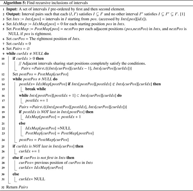
C.3. The algorithm — projected occurrences to Prokrustean graph

The algorithm below reduces the task of reconstructing the Prokrustean graph from ${ProjOcc}_{𝒰}$ to a problem designed for a specific string $S\in 𝒰$. For the subset of regions $\left\{\left(S^{\prime },i,j\right)\in {ProjOcc}_{𝒰}\mid S^{\prime }=S\right\}$, determine their inclusion relationships to identify the closest related pairs. This is easily parallelized as it processes the intervals for each $S$ separately. And the running time is linear to the size of the subset of regions per each $S$, hence |${ProjOcc}_{𝒰}$| in total.

An important assumption in the algorithm is that for any region $(S,i,j)\in {ProjOcc}_{𝒰}$, within the subset $\{\left(S^{\prime },i,j\right)\in {ProjOcc}_{𝒰}\mid S^{\prime }=S\}$, there are at most two regions $\left(S,i^{\prime },j^{\prime }\right)$ such that $(S,i,j)⊊\left(S,i^{\prime },j^{\prime }\right)$ and no $(S,x,y)$ exists where $(S,i,j)⊊(S,x,y)⊊\left(S,i^{\prime },j^{\prime }\right)$. It is straightforward to check the property.

References

- [1].AlEisa Hussah N, Hamad Safwat, and Elhadad Ahmed. K-mer spectrum-based error correction algorithm for next-generation sequencing data. Computational Intelligence and Neuroscience, 2022, 2022. [DOI] [PMC free article] [PubMed] [Google Scholar]
- [2].Balvert Marleen, Luo Xiao, Hauptfeld Ernestina, Schönhuth Alexander, and Dutilh Bas E. Ogre: overlap graph-based metagenomic read clustering. Bioinformatics, 37(7):905–912, 2021. [DOI] [PMC free article] [PubMed] [Google Scholar]
- [3].Bankevich Anton, Bzikadze Andrey V, Kolmogorov Mikhail, Antipov Dmitry, and Pevzner Pavel A. Multiplex de bruijn graphs enable genome assembly from long, high-fidelity reads. Nature biotechnology, 40(7):1075–1081, 2022. [DOI] [PubMed] [Google Scholar]
- [4].Belazzougui Djamal. Linear time construction of compressed text indices in compact space. In Proceedings of the forty-sixth Annual ACM Symposium on Theory of Computing, pages 148–193, 2014. [Google Scholar]
- [5].Belazzougui Djamal and Cunial Fabio. Fully-functional bidirectional burrows-wheeler indexes and infinite-order de bruijn graphs. In 30th Annual Symposium on Combinatorial Pattern Matching (CPM 2019). Schloss Dagstuhl-Leibniz-Zentrum fuer Informatik, 2019. [Google Scholar]
- [6].Beller Timo, Gog Simon, Ohlebusch Enno, and Schnattinger Thomas. Computing the longest common prefix array based on the burrows–wheeler transform. Journal of Discrete Algorithms, 18:22–31, 2013. [Google Scholar]
- [7].Benoit Gaëtan. Simka: fast kmer-based method for estimating the similarity between numerous metagenomic datasets. In RCAM, 2015. [Google Scholar]
- [8].Besta Maciej, Kanakagiri Raghavendra, Mustafa Harun, Karasikov Mikhail, Rätsch Gunnar, Hoefler Torsten, and Solomonik Edgar. Communication-efficient jaccard similarity for high-performance distributed genome comparisons. In 2020 IEEE International Parallel and Distributed Processing Symposium (IPDPS), pages 1122–1132. IEEE, 2020. [Google Scholar]
- [9].Bonnici Vincenzo and Manca Vincenzo. Informational laws of genome structures. Scientific reports, 6(1):28840, 2016. [DOI] [PMC free article] [PubMed] [Google Scholar]
- [10].Bonnie Jessica K, Ahmed Omar, and Langmead Ben. Dandd: efficient measurement of sequence growth and similarity. bioRxiv, pages 2023–02, 2023. [DOI] [PMC free article] [PubMed] [Google Scholar]
- [11].Boucher Christina, Bowe Alex, Gagie Travis, Puglisi Simon J, and Sadakane Kunihiko. Variable-order de bruijn graphs. In 2015 data compression conference, pages 383–392. IEEE, 2015. [Google Scholar]
- [12].Bowe Alexander, Onodera Taku, Sadakane Kunihiko, and Shibuya Tetsuo. Succinct de bruijn graphs. In International workshop on algorithms in bioinformatics, pages 225–235. Springer, 2012. [Google Scholar]
- [13].Breitwieser Florian P, Baker Daniel N, and Salzberg Steven L. Krakenuniq: confident and fast metagenomics classification using unique k-mer counts. Genome biology, 19:1–10, 2018. [DOI] [PMC free article] [PubMed] [Google Scholar]
- [14].Břinda Karel, Baym Michael, and Kucherov Gregory. Simplitigs as an efficient and scalable representation of de bruijn graphs. Genome biology, 22:1–24, 2021. [DOI] [PMC free article] [PubMed] [Google Scholar]
- [15].Bussi Yuval, Kapon Ruti, and Reich Ziv. Large-scale k-mer-based analysis of the informational properties of genomes, comparative genomics and taxonomy. PloS one, 16(10):e0258693, 2021. [DOI] [PMC free article] [PubMed] [Google Scholar]
- [16].Cavattoni Margherita and Comin Matteo. Classgraph: improving metagenomic read classification with overlap graphs. Journal of Computational Biology, 30(6):633–647, 2023. [DOI] [PubMed] [Google Scholar]
- [17].Cenzato Davide, Guerrini Veronica, Lipták Zsuzsanna, and Rosone Giovanna. Computing the optimal BWT of very large string collections. In In Proc. of the 33rd Data Compression Conference, DCC 2023, 2023, pages 71–80, 2023. doi: 10.1109/DCC55655.2023.00015. [DOI] [Google Scholar]
- [18].Cenzato Davide and Lipták Zsuzsanna. A survey of bwt variants for string collections. Bioinformatics, page btae333, 2024. [DOI] [PMC free article] [PubMed] [Google Scholar]
- [19].Chikhi Rayan and Medvedev Paul. Informed and automated k-mer size selection for genome assembly. Bioinformatics, 30(1):31–37, 2014. [DOI] [PubMed] [Google Scholar]
- [20].Cracco Andrea and Tomescu Alexandru I. Extremely fast construction and querying of compacted and colored de bruijn graphs with ggcat. Genome Research, pages gr–277615, 2023. [DOI] [PMC free article] [PubMed] [Google Scholar]
- [21].Díaz-Domínguez Diego and Navarro Gonzalo. Efficient construction of the bwt for repetitive text using string compression. Information and Computation, 294:105088, 2023. [Google Scholar]
- [22].D’ıaz-Dom’ınguez Diego, Onodera Taku, Puglisi Simon J, and Salmela Leena. Genome assembly with variable order de bruijn graphs. bioRxiv, pages 2022–09, 2022. [Google Scholar]
- [23].Dubinkina Veronika B, Ischenko Dmitry S, Ulyantsev Vladimir I, Tyakht Alexander V, and Alexeev Dmitry G. Assessment of k-mer spectrum applicability for metagenomic dissimilarity analysis. BMC bioinformatics, 17:1–11, 2016. [DOI] [PMC free article] [PubMed] [Google Scholar]
- [24].Gog Simon, Beller Timo, Moffat Alistair, and Petri Matthias. From theory to practice: Plug and play with succinct data structures. In 13th International Symposium on Experimental Algorithms, (SEA 2014), pages 326–337, 2014. [Google Scholar]
- [25].Gusfield Dan. Algorithms on stings, trees, and sequences: Computer science and computational biology. Acm Sigact News, 28(4):41–60, 1997. [Google Scholar]
- [26].Irber Luiz, Brooks Phillip T, Reiter Taylor, Tessa Pierce-Ward N, Hera Mahmudur Rahman, Koslicki David, and Titus Brown C. Lightweight compositional analysis of metagenomes with fracminhash and minimum metagenome covers. bioRxiv, pages 2022–01, 2022. [Google Scholar]
- [27].Islam Rashedul, Raju Rajan Saha, Tasnim Nazia, Shihab Istiak Hossain, Bhuiyan Maruf Ahmed, Araf Yusha, and Islam Tofazzal. Choice of assemblers has a critical impact on de novo assembly of sars-cov-2 genome and characterizing variants. Briefings in bioinformatics, 22(5):bbab102, 2021. [DOI] [PMC free article] [PubMed] [Google Scholar]
- [28].Kokot Marek, Długosz Maciej, and Deorowicz Sebastian. Kmc 3: counting and manipulating k-mer statistics. Bioinformatics, 33(17):2759–2761, 2017. [DOI] [PubMed] [Google Scholar]
- [29].Krannich Thomas, Timothy J White W, Niehus Sebastian, Holley Guillaume, Halldórsson Bjarni V, and Kehr Birte. Population-scale detection of non-reference sequence variants using colored de bruijn graphs. Bioinformatics, 38(3):604–611, 2022. [DOI] [PMC free article] [PubMed] [Google Scholar]
- [30].Li Heng. Fast construction of fm-index for long sequence reads. Bioinformatics, 30(22):3274–3275, 2014. [DOI] [PMC free article] [PubMed] [Google Scholar]
- [31].Liao Xingyu, Li Min, Luo Junwei, Zou You, Wu Fang-Xiang, Pan Yi, Luo Feng, and Wang Jianxin. Improving de novo assembly based on read classification. IEEE/ACM Transactions on Computational Biology and Bioinformatics, 17(1):177–188, 2018. [DOI] [PubMed] [Google Scholar]
- [32].Mallawaarachchi Vijini. Metagenomics Binning Using Assembly Graphs. PhD thesis, The Australian National University (Australia), 2022. [Google Scholar]
- [33].Nurk Sergey, Meleshko Dmitry, Korobeynikov Anton, and Pevzner Pavel A. metaspades: a new versatile metagenomic assembler. Genome research, 27(5):824–834, 2017. [DOI] [PMC free article] [PubMed] [Google Scholar]
- [34].Ondov Brian D, Treangen Todd J, Melsted Páll, Mallonee Adam B, Bergman Nicholas H, Koren Sergey, and Phillippy Adam M. Mash: fast genome and metagenome distance estimation using minhash. Genome biology, 17:1–14, 2016. [DOI] [PMC free article] [PubMed] [Google Scholar]
- [35].Pérez-Cobas Ana Elena, Gomez-Valero Laura, and Buchrieser Carmen. Metagenomic approaches in microbial ecology: an update on whole-genome and marker gene sequencing analyses. Microbial genomics, 6(8):e000409, 2020. [DOI] [PMC free article] [PubMed] [Google Scholar]
- [36].Ponsero Alise Jany, Miller Matthew, and Hurwitz Bonnie Louise. Comparison of k-mer-based de novo comparative metagenomic tools and approaches. Microbiome Research Reports, 2(4), 2023. [DOI] [PMC free article] [PubMed] [Google Scholar]
- [37].Prezza Nicola and Rosone Giovanna. Space-efficient computation of the lcp array from the burrows-wheeler transform. arXiv preprint arXiv:1901.05226, 2019. [Google Scholar]
- [38].Prjibelski Andrey, Antipov Dmitry, Meleshko Dmitry, Lapidus Alla, and Korobeynikov Anton. Using spades de novo assembler. Current protocols in bioinformatics, 70(1):e102, 2020. [DOI] [PubMed] [Google Scholar]
- [39].Rhyker Ranallo-Benavidez T, Jaron Kamil S, and Schatz Michael C. Genomescope 2.0 and smudgeplot for reference-free profiling of polyploid genomes. Nat. comm., 11(1):1432, 2020. [DOI] [PMC free article] [PubMed] [Google Scholar]
- [40].Rizzi Raffaella, Beretta Stefano, Patterson Murray, Pirola Yuri, Previtali Marco, Vedova Gianluca Della, and Bonizzoni Paola. Overlap graphs and de bruijn graphs: data structures for de novo genome assembly in the big data era. Quantitative Biology, 7:278–292, 2019. [Google Scholar]
- [41].Rodriguez-r Luis M and Konstantinidis Konstantinos T. Estimating coverage in metagenomic data sets and why it matters. The ISME journal, 8(11):2349–2351, 2014. [DOI] [PMC free article] [PubMed] [Google Scholar]
- [42].Schmidt Sebastian, Khan Shahbaz, Alanko Jarno N, Pibiri Giulio E, and Tomescu Alexandru I. Matchtigs: minimum plain text representation of k-mer sets. Genome Biology, 24(1):136, 2023. [DOI] [PMC free article] [PubMed] [Google Scholar]
- [43].Shariat Basir, Movahedi Narjes Sadat, Chitsaz Hamidreza, and Boucher Christina. Hyda-vista: towards optimal guided selection of k-mer size for sequence assembly. BMC genomics, 15(10):1–8, 2014. [DOI] [PMC free article] [PubMed] [Google Scholar]
- [44].Tang Deyou, Li Yucheng, Tan Daqiang, Fu Juan, Tang Yelei, Lin Jiabin, Zhao Rong, Du Hongli, and Zhao Zhongming. Kcoss: an ultra-fast k-mer counter for assembled genome analysis. Bioinformatics, 38(4):933–940, 2022. [DOI] [PubMed] [Google Scholar]
- [45].Wickramarachchi Anuradha and Lin Yu. Metagenomics binning of long reads using read-overlap graphs. In RECOMB International Workshop on Comparative Genomics, pages 260–278. Springer, 2022. [Google Scholar]
- [46].Yang Zhenhua, Li Hong, Jia Yun, Zheng Yan, Meng Hu, Bao Tonglaga, Li Xiaolong, and Luo Liaofu. Intrinsic laws of k-mer spectra of genome sequences and evolution mechanism of genomes. BMC Evolutionary Biology, 20:1–15, 2020. [DOI] [PMC free article] [PubMed] [Google Scholar]
- [47].Zhai Hongxuan and Fukuyama Julia. A convenient correspondence between k-mer-based metagenomic distances and phylogenetically-informed β-diversity measures. PLOS Computational Biology, 19(1):e1010821, 2023. [DOI] [PMC free article] [PubMed] [Google Scholar]