Evaluating Geographical Health Disparities in Cancer Care: Example of the Modifiable Areal Unit Problem

Introduction

As geographic information systems become more accessible to researchers, the role of geography in health research is becoming increasingly salient¹ and can lead to misapplication of important geographic concepts. One such example is the “Modifiable Areal Unit Problem” (MAUP), a type of ecological fallacy which can lead to different results depending on the areal unit chosen for analysis.² This may disproportionately impact rural areas compared to urban areas, with the former suffering from highly variable rates for the same area due to lower population density. To truly understand how geography affects health outcomes, we must understand how the units of analysis we select impact our results. In this analysis, we demonstrate the differences in results stemming from our use of differing areal units for evaluating disparities in late-stage presentation for patients with breast cancer.

Methods

We identified patients with incident breast cancer within the Indiana State Cancer Registry from 2010 to 2015. The geospatial heterogeneity of late-stage breast cancer was analyzed at three different geographical levels: county, census tract, and block group. Counties are administrative entities that vary widely in both area and population size. Census tracts are statistical subdivisions of a county with a target population of 4,000 inhabitants.³ Block groups are subdivisions of a census tract containing between 600 and 3,000 people. The Global Moran’s I statistic was used to investigate overall clustering of location.⁴ We illustrate the potential impact of using different areal units with maps of rates of late-stage breast cancer at each level across Indiana. Given the de-identified nature of the Indiana State Cancer Registry dataset, the study was exempt from IRB review. Areas where case counts were fewer than 6 were “suppressed” and not shown on the map out of privacy concerns.

Results

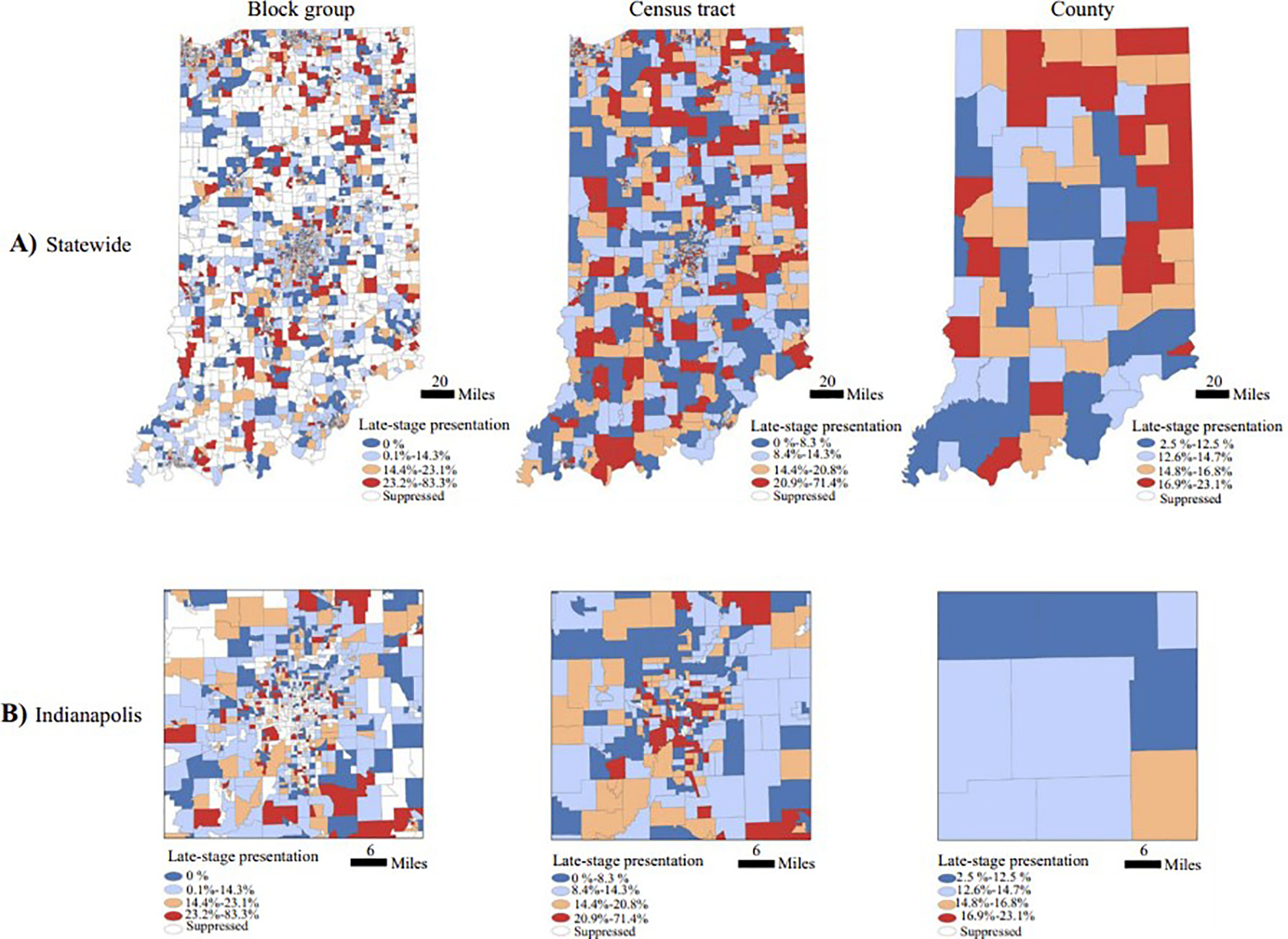
Our sample included 30,604 patients with breast cancer residing in 4,814 block groups, 1,511 census tracts, and 92 counties. We observed similar proportion of late-stage presentation at the level of block group (15.2%), census tract (15.3%), and county (14.5%). At the block group level, low case counts led to highly variable rates and suppression of data presentation (Figure 1). At the county level, we were unable to appreciate local variation in late-stage presentation rates. For example, maps of areas of low rates at the county level (such as Indianapolis) obscured the high rates of late-stage presentation visible within the county at the census tract level. Our analysis showed decreasing variance and spatial autocorrelation with increasing size of area and loss of statistical significance when evaluating at the level of county (Table 1).

Figure 1.

Percentage of patients presenting with late-stage breast cancer in Indiana from 2010 to 2015. This figure shows rates of late-stage presentation for breast cancer at the block group level, census tract level, and county level throughout the state of Indiana (first row) and Indianapolis (2nd row). Rates for areal units with case counts <6 were suppressed

Table 1.

Mean rates of late-stage presentation and clustering measurement by areal unit. A Global Moran’s Index of 0 indicates no autocorrelation, 1 indicates perfect clustering and −1 indicates perfect dispersion.

	Block group	Census tract	County
Mean rate	15.2%	15.3%	14.3%
Variance	19.1	11.0	3.8
Global Moran’s Index	0.02	0.04	0.09
p-value	<0.001	<0.001	0.19

Discussion

Understanding how rates of late-stage breast cancer vary geographically is essential for formulating and targeting interventions. We found that using block group-level data prevented meaningful evaluation of rate changes due to small denominators, whereas using county-level data obscured potentially important within-county differences. These analyses show the importance of empirically examining the impact of selecting different areal units rather than simply using whichever areal unit available in a given dataset. Health services researchers are increasingly using different area-level measures of socioeconomic factors and should consider the implications of the areal unit being applied, including unstable rates with small populations or masking of heterogeneity with larger areas.⁵ Researchers should also explore alternative methods that minimize MAUP. For example, the Restricted and Controlled Monte Carlo process disaggregates polygon-level data (such as block group, census tract, or county) to achieve mapping aggregate data at an approximated individual level based on pre-existing population distributions, transforming area-based data into point-based data and thus avoiding the MAUP.⁶ Given the potential for inconsistent if not conflicting results, spatial analyses must thoughtfully approach the most appropriate, accurate, and stable methods when evaluating geospatial differences in care.

References:

- 1.Wang F Why Public Health Needs GIS: A Methodological Overview. Ann GIS. 2020;26(1):1–12. Epub 2019 Dec 19. [DOI] [PMC free article] [PubMed] [Google Scholar]
- 2.Openshaw S The Modifiable Areal Unit Problem; Geo Books: Norwich, UK, 1984. [Google Scholar]
- 3.United States Census Bureau. Glossary. Accessed on 3/2/2023 at: https://www.census.gov/programs-surveys/geography/about/glossary.html.
- 4.Jerrett M, Gale S, Kontgis C. Spatial modeling in environmental and public health research. Int J Environ Res Public Health. 2010;7(4):1302–1329. [DOI] [PMC free article] [PubMed] [Google Scholar]
- 5.Markey C, Bello O, Hanley M, Loehrer AP. The use of area-level socioeconomic indices in evaluating cancer care delivery – A Scoping Review. Ann Surg Oncol. 2023; Online ahead of print. doi: 10.1245/s10434-023-13099-x. [DOI] [PMC free article] [PubMed] [Google Scholar]
- 6.Shi X, Miller S, Mwenda K, Onda A, Reese J, Onega T, Gui J, Karagas M, Demidenko E, Moeschler J. Mapping disease at an approximated individual level using aggregate data: a case study of mapping New Hampshire birth defects. Int J Environ Res Public Health. 2013. Sep 6;10(9):4161–74. [DOI] [PMC free article] [PubMed] [Google Scholar]