Abstract
Four-dimensional computed tomography (4D-CT) plays an important role in lung cancer treatment because of its capability in providing a comprehensive characterization of respiratory motion for high-precision radiation therapy. However, due to the inherent high-dose exposure associated with CT, dense sampling along superior–inferior direction is often not practical, thus resulting in an inter-slice thickness that is much greater than in-plane voxel resolutions. As a consequence, artifacts such as lung vessel discontinuity and partial volume effects are often observed in 4D-CT images, which may mislead dose administration in radiation therapy. In this paper, we present a novel patch-based technique for resolution enhancement of 4D-CT images along the superior–inferior direction. Our working premise is that anatomical information that is missing in one particular phase can be recovered from other phases. Based on this assumption, we employ a hierarchical patch-based sparse representation mechanism to enhance the superior–inferior resolution of 4D-CT by reconstructing additional intermediate CT slices. Specifically, for each spatial location on an intermediate CT slice that we intend to reconstruct, we first agglomerate a dictionary of patches from images of all other phases in the 4D-CT. We then employ a sparse combination of patches from this dictionary, with guidance from neighboring (upper and lower) slices, to reconstruct a series of patches, which we progressively refine in a hierarchical fashion to reconstruct the final intermediate slices with significantly enhanced anatomical details. Our method was extensively evaluated using a public dataset. In all experiments, our method outperforms the conventional linear and cubic-spline interpolation methods in preserving image details and also in suppressing misleading artifacts, indicating that our proposed method can potentially be applied to better image-guided radiation therapy of lung cancer in the future.
Keywords: Adaptive dictionary, four-dimensional computed tomography (4D-CT) lung data, hierarchical patch-based sparse representation, resolution enhancement
I. Introduction
For decades, determining the accurate radiation dose for a moving target in the lung, such as a tumor, has been an extremely challenging problem in cancer radiation therapy [1], [2]. Information used for guiding treatment planning and delivery typically comes from images acquired using free-breathing three-dimensional computed tomography, with no isolated respiratory phase information. This essentially implies the absence of motion information in aiding the estimation of volume and shape of the moving structures in the lung. Thus, to ensure sufficient tumor coverage, an estimated tumor region is generally expanded in all directions to account for target motion. This unnecessary enlargement of the treatment target volume can result in harm to the healthy tissue.
With four-dimensional computed tomography (4D-CT), additional phased images can help capture respiratory motion information that is crucial for target definition in radiation therapy. 4D-CT is usually obtained by sorting the multiple free-breathing CT segments in relation to the couch position and the tidal volume [3], [4]. Due to the risk of radiation [5], [6], only a limited number of CT segments are usually acquired, resulting in much lower inter-slice resolution when compared with the in-plane resolution. This lack of sufficient structural information along the superior–inferior direction introduces image artifacts such as vessel discontinuity and partial voluming. Consequently, correct assessment of tumor could be severely affected due to shape distortion. Fig. 1 shows the example coronal and sagittal views of 4D-CT lung data. Due to the lower superior–inferior resolution (5 mm), many structural details are not observable.
Fig. 1.

Example coronal and sagittal views of 4D-CT lung data.
The main objective of this paper is to enhance the image quality of 4D-CT, in order to help treatment planning for radiation therapy. The respiratory phase information afforded by 4D-CT is important for the estimation of lung motion trajectory for more accurate administration of radiation therapy without incurring unnecessary radiation dose. However, due to the inherent high-dose exposure associated with CT, dense sampling along the superior–inferior direction is often not practical, thus resulting in an inter-slice thickness that is much greater than in-plane voxel resolutions. Many recent studies have attempted to improve the resolution of lung 4D-CT data. For example, an optical flow based temporal interpolation technique [7], [8] has been proposed to reduce the motion artifact of 4D-CT data. To reduce the scan dose, a temporal nonlocal mean strategy was employed in [9] to regularize the reconstruction of 4D-CT with undersampled projections. In [10] and [11], a registration-based approach was also applied to interpolate intermediate phases based on a couple of reference phases (e.g., inhale and exhale phases). Although this increases the number of phases in the 4D-CT image sequence, it does not increase the actual inter-slice resolution.
A commonly used approach to increase inter-slice resolution is interpolation. Grevera et al. [12] summarized interpolation methods into two groups: scene-based and object-based methods. For scene-based approaches, interpolation is performed based on image intensity. Linear and spline-based interpolation methods are the commonly used scene-based methods due to their simplicity. However, scene-based approaches suffer from significant shift of anatomical patterns between neighboring slices, causing undesirable artifacts and blurred edges [13].
Object-based interpolation methods extract additional information to guide interpolation, which include shape-based [12], morphology-based [14], optical-flow-based [15], [16], and registration-based approaches [13], [17]. These methods are based on an important assumption: anatomical structures are similar between neighboring slices. While this assumption is generally true for the brain, abdomen, and teeth, the lung CT interpolation is a difficult problem where structural shapes vary rapidly and hence could be very different across slices.
An alternative approach is to reconstruct a high resolution image by combining low resolution images [18]. Several super-resolution methods have been proposed for generating high-resolution medical images [19]–[24]. In general, these methods take an image restoration approach by estimating the point spread function (PSF) associated with image blurring, down-sampling, and subject motion, and together with a regularization term (i.e., Tikhonov cost function, Total variation, Gibbs prior, etc.) optimize an appropriately defined energy function to recover the super-resolution image. For instance, Greenspan et al. [19], [21] proposed an approach for MRI image super-resolution reconstruction that is based on the Irani–Peleg back projection (BP) model [25], via estimation of the PSF associated with subject motion. Gholipour et al. [23] combined maximum likelihood estimation and robust M-estimation to build super-resolution volume data for fetal brain MRI. Wallach et al. [26] implemented maximum a posteriori (MAP) algorithm to reconstruct respiratory high-resolution synchronized PET data, where the Huber regularization term was used to ensure convergence and also the B-spline registration was used for motion estimation. Recently, Rousseau [20] proposed a nonlocal approach for image super-resolution using inter-modality priors. The high-resolution brain image was generated from an input low-resolution image with the help of priors obtained from another high resolution brain image. For the above approaches, PSF estimation has direct influence on the super-resolution reconstruction, and yet it is nontrivial and often error-prone to estimate.
In this work, we will develop a novel method to enhance the resolution of 4D-CT by taking into consideration the important fact that during the course of 4D-CT acquisition, complementary anatomical information is spread throughout different phases. By using this complementary information, our approach will reconstruct intermediate slices to increase the resolution of 4D-CT beyond the acquired resolution. Our method infers structural details in the intermediate slices in a patch-by-patch fashion by considering the dictionaries of patches generated adaptively from the images at other phases. Patches in these dictionaries are combined using a hierarchical sparse representation framework to form the most representative patches in relation to the neighborhood of the target patches. Note that Tian et al. have also used interphase information to improve 4D-CT reconstruction [9]. In their work, the interphase correlation between images at successive phases is captured via a nonlocal means mechanism for regularizing the reconstruction of 4D-CT from undersampled projection data. In other words, the interphase correlation is used only to constrain the 4D-CT reconstruction so that the reconstruction results for the similar structures could be consistent across different phases. Our work solves a different problem with a fundamentally different approach. In our work, the interphase information is carried across phases for intermediate slice reconstruction, not merely for regularization.
A preliminary version of this work was presented in [27]. The preliminary framework is extended in this work to incorporate a hierarchical refinement mechanism where image structural details are recovered from a coarse-to-fine fashion. With this improvement, we are able to recover greater structural details and at the same time deal with blocking artifacts. Experimental validation is also substantially extended to evaluate performance of the proposed framework more comprehensively.
Patch-based sparse representation has recently attracted rapidly growing interest. This approach assumes that image patches can be represented by a sparse linear combination of an overcomplete dictionary of image patches. This strategy has been applied to a good deal of image processing problems, such as image denoising [28], [29], image in-painting [30], color image restoration [29], image recognition [31], [32], achieving state-of-the-art performance. Yang et al. [33] showed that the high-resolution images can be achieved by using sparse representation. Tosic et al. [34] enhanced the breast ultrasound image resolution based on the dictionary trained from the high-resolution MRI dataset. Chen et al. [35] employed the dictionary trained using prior information to improve the accuracy in MRI reconstruction, from significantly undersampled data. Ravishankar et al. [36] further proposed an MRI image reconstruction method from the highly undersampled k-space data, and then built high-resolution MRI images with the help of specific dictionary that was trained from the complete k-space data. These studies demonstrate the potential applications of sparse representation in improving the resolution of medical images.
The general formulation of sparse representation can be described as follows. Let be an overcomplete dictionary of prototype signal-atoms. A signal can be represented by or approximately as , satisfying . The vector , which has few nonzero values, is comprised of the sparse coefficients needed to reconstruct the signal . To solve for , both and a dictionary are needed. For the application such as denoising and deblurring, represents the observed degraded image, and is a learned universal dictionary. In our case, is not available and needs to be reconstructed. We use neighboring image information in place of to help estimate (see Section III for details). In addition, we note that building a “global” dictionary that caters for the whole lung is computationally intractable. Thus, we resort to building individual dictionaries that will adapt to the structural patterns of local image patches.
The proposed approach can be divided into two steps. In the first step, a patch-based sparse-representation formulation is built to reconstruct the initial intermediate slices. In the second step, a hierarchical approach is used to iteratively refine the initial results. Compared with conventional linear and cubic spline interpolation methods, we will show that our method yields superior performance both qualitatively and quantitatively. We will present details of our method for enhancing the resolution of lung 4D-CT in Section II. Results on extensive evaluation of the proposed method in comparison with the conventional interpolation methods will be provided in Section III. Section IV concludes this paper.
II. Method
A. Basic Idea
Our key assumption is that image information lost in one respiratory phase will appear in other phases. This is illustrated in Fig. 2. The blue solid horizontal lines indicate the scanned slices. The blue dashed horizontal line indicates the intermediate slice that needs to be reconstructed. During different respiratory phases, the lung moves in the superior–inferior direction and information pertaining to the intermediate slice might be captured in the scans of other phases.
Fig. 2.
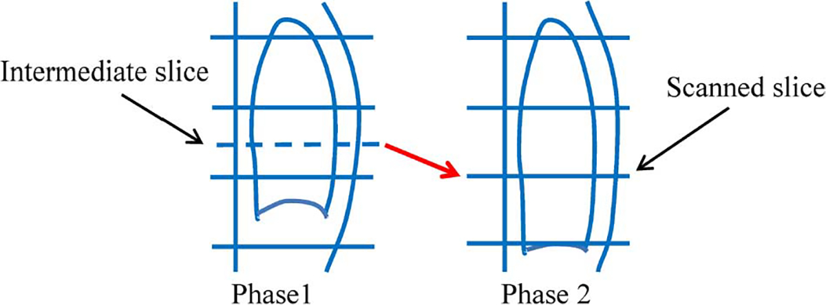
Recovering image information from scans of different respiratory phases. Blue solid horizontal lines indicate actual scanned CT slices. Blue dashed line indicates intermediate slice that needs to be reconstructed. Due to respiratory motion, information needed to reconstruct intermediate slice in Phase 1 may be captured in Phase 2, i.e., slice pointed by the red arrow.
B. Method Overview
Given the acquired 4D-CT images , where is the number of phases and is the total number of slices in each phase image , the goal is to reconstruct an intermediate high-resolution slice between two consecutive slices and in image . The major concepts involved in our method are illustrated in Fig. 3. The blue solid and dashed lines in the figure denote the existing slices and the intermediate slices to be reconstructed, respectively. Since the scanning time for each slice is relatively fast (< 0.1 sec), we regard each slice to be free of motion artifacts. For capturing local anatomical nuances, we further divide the intermediate slice into a number of overlapping patches. For each patch (red box in Fig. 3), we assume that the missing structural details that are to be recovered can be found in other phases (purple boxes in Fig. 3). Thus, the estimation of patches on the intermediate slice can be formulated as the problem of finding linear combinations of patches from a patch dictionary gathered from complimentary respiratory phases. To achieve this, two problems have to be solved. 1) How should the dictionary for each patch be constructed? 2) How do we find the best representation based on the dictionary? Our proposed solutions to these problems will be discussed next. A summary of the mathematical notations involved in this paper is provided in Table I.
Fig. 3.

Overview of our patch-based method for enhancing resolution of 4D-CT. Patch of interest (red box) on an intermediate slice (blue dashed line) is estimated by seeking a sparse combination of anatomically similar patches from other phases (purple boxes).
TABLE I.
Summary of Notations
| Notation | Description |
|---|---|
|
| |
| The intermediate slice that needs to be reconstructed | |
| Composing patches of | |
| Patches immediately superior and inferior to | |
| The reconstructed intermediate slice at each iteration | |
| Composing patches of | |
| Dictionary for sparse representation | |
| Threshold for sparse representation | |
| Tuning parameter between the contributions of image intensity and image feature | |
| Parameter for controlling the global constraint | |
C. Construction of Motion Adaptive Dictionaries
Patch-based dictionary learning is widely used in computer vision for image denoising and super-resolution [28], [29], [33], [37]. The key requirement in constructing an effective dictionary is that the dictionary should be universal enough to represent every possible patch with sufficient accuracy. To achieve this, typically hundreds of thousands of patches are required to learn a “global” dictionary [33]. This approach will, however, require a significantly larger amount of computation to reconstruct each patch since all patches in this large global dictionary will have to be consulted during the reconstruction process. Moreover, not all patches in this global dictionary are necessary for the reconstruction of the patch of interest. Due to these reasons, we have opted to construct smaller dictionaries that can better adapt to each local patch.
Assuming that the space of an intermediate slice has been divided into overlapping patches, we use , a column vector (red box in Fig. 4), to denote the intensity values of an arbitrary patch at phase . The search for patches to be included in the dictionary is based on adaptive bounding boxes for images at phases , using patches immediately superior and inferior to , denoted as and , as references (see two purple boxes in phase of Fig. 4). Since lung motion is predominantly along the superior–inferior direction, patch searching in the left-right and anterior–posterior directions is restricted. The search range is adjusted in the superior–inferior direction based on the fact that lung motion near the diaphragm is significantly larger than locations that are far away. For each image at phase , we extract with respect to a dictionary matrix (see purple boxes in phase of Fig. 4), where is the length of , and is the number of voxels within the bounding box set for the image at phase . We repeat this for all phases to construct the final dictionary matrix , where .
Fig. 4.

Construction of an adaptive dictionary for a particular patch (red box) in intermediate slice at phase . Search bounding box is adaptively determined at each phase by using immediate superior and inferior patches (purple box) as references. After determining the bounding box at each phase, all possible patches (purple boxes) across different phases are included into the dictionary .
D. Hierarchical Patch-Based Intermediate Slice Reconstruction by Sparse Representation
First Step: Reconstructing Initial Intermediate Slices:
a). General Formulation:
Upon obtaining the relevant dictionary for patch , the next task is to find a suitable reconstruction strategy using the dictionary. In this work, the estimation of is formulated as the linear combination of patches in the dictionary, i.e., , where is a weight vector (column vector). The patches and , immediately superior and inferior to , are used as constraints for the initial reconstruction of . This is discussed with more detail in the following.
First, the reconstructed patch should resemble both and
| (1) |
where is a threshold for controlling patch discrepancy. In addition, we require that the reconstructed patch is not biased towards any of these two consecutive patches, i.e., and should be balanced
| (2) |
where is a tolerance factor, with value ranged from 1.1 to 2.3.
For better characterization of structural patterns in the patches, we use both the original intensity values and the derived features to represent each patch. Thus, (1) and (2) can be modified to
| (3) |
and
| (4) |
where and are the new dictionary and new patch, as defined by is the feature operator, which in our case computes the gradients based on the intensity values. is a tuning parameter that controls the balance between the contributions of image intensity and image feature. The augmented distance conditions then become
| (5) |
Second, the weight vector should be sparse. Including more than necessary patches from the dictionary will only marginally reduce the fitting error in (5) at the expense of adding noise and blur to the reconstructed lung anatomy. We, therefore, penalize the weight vector using the -norm, , and reformulate the optimization problem to become
| (6) |
and
b). Numerical Solution for Sparse Representation:
We use an efficient algorithm to find the sparse representation (or ) in a greedy fashion. Similar to the matching pursuit algorithm [38], [39], we sequentially select nonzero-weighted atoms from the dictionary . Let denote element/atom in dictionary . We denote the set of selected atoms at iteration as , where indicates the index of the atom selected at the th iteration. The weight vector at iteration is a function of , i.e., , all elements in are zero except . The estimate of at iteration is then . The next atom is selected so that we have (7), as shown at bottom of page, and
As explained in the Appendix, the optimization problem associated with (7) can be solved using an approach that is similar to locally linear embedding (LLE) [40]. The process above is iterated until falls below a certain threshold [see (6)] or when it starts to increase.
Fig. 5 shows an example reconstructed slice. From left to right, the ground truth, the results given by linear interpolation, cubic-spline interpolation, and our proposed method are shown, respectively. It can be seen that our method achieves the best result with the least amount of artifacts and the greatest similarity with the ground truth. More results will be reported in the experiment section.
Fig. 5.

Example of reconstructed slice. Ground truth and results given by linear interpolation, cubic-spline interpolation, and our method are shown from left to right, respectively. Our method shows the best result, especially in circled areas.
c). Parameter Determination:
To achieve the best reconstruction for the initial resolution-enhanced images, several critical parameters need to be fine-tuned: patch size, patch overlap, parameter , and parameter . We use three typical cases (case3, case4, and case7 from the DIR-lab [41]) to test the influence of each parameter. The details of the experiment data, software, and hardware platform will be described in Section III-A.
Local Patch Size and Overlap Degree:
Fig. 6 shows the average peak signal-to-noise ratio (PSNR) for intermediate slice reconstruction with respect to the use of different patch size and overlap degree. Although speeding up computation (see Table II), the low overlap degree between two patches introduces significant blocking artifacts. Given the same patch size, the reconstruction with larger patch overlap always gives better results along with less artifacts. We note, however, large overlap increases computation time dramatically (e.g. 16/12 and 32/28). The patch size also has significant influence on the results. As shown in Fig. 6, the average PSNR increases with the increase of patch size from 8 × 8 to 32 × 32. This is not surprising since large local patches can capture more anatomical information for robust matching. Based on these analyses, as a tradeoff between the computational speed and accuracy, we set patch size to 32 with 24 pixels overlap for the first step of our approach throughout all the experiments presented in Sections III-C and III-D.
Fig. 6.

Influence of patch size and patch overlap. For -axis, 8/4 denotes a patch size of 8 × 8 with four overlapping pixels in each dimension, and so forth. Computation times for three highest PSNR values are provided. See Table II for the rest of the computation times.
TABLE II.
Average Computation Time Per Slice
| Patch size | Patch Overlap | Computation Time |
|---|---|---|
|
| ||
| 8 × 8 | 4 pixels | 187.86 sec/slice |
| 8 × 8 | 6 pixels | 877.84 sec/slice |
| 16 × 16 | 8 pixels | 50.19 sec/slice |
| 16 × 16 | 12 pixels | 263.16 sec/slice |
| 32 × 32 | 16 pixels | 17.72 sec/slice |
| 32 × 32 | 24 pixels | 67.99 sec/slice |
| 32 × 32 | 28 pixels | 224.36 sec/slice |
| 48 × 48 | 40 pixels | 98.80 sec/slice |
| 48 × 48 | 44 pixels | 394.92 sec/slice |
Parameter :
Recall that the balance between image intensities and image features is controlled by the parameter . Fig. 7 shows the average PSNR values with changing from 0 to 1.2 for three different cases. It is clear that provides the best reconstruction result in terms of PSNR. We, therefore, set throughout all experiments presented in Sections III-C and III-D.
Fig. 7.
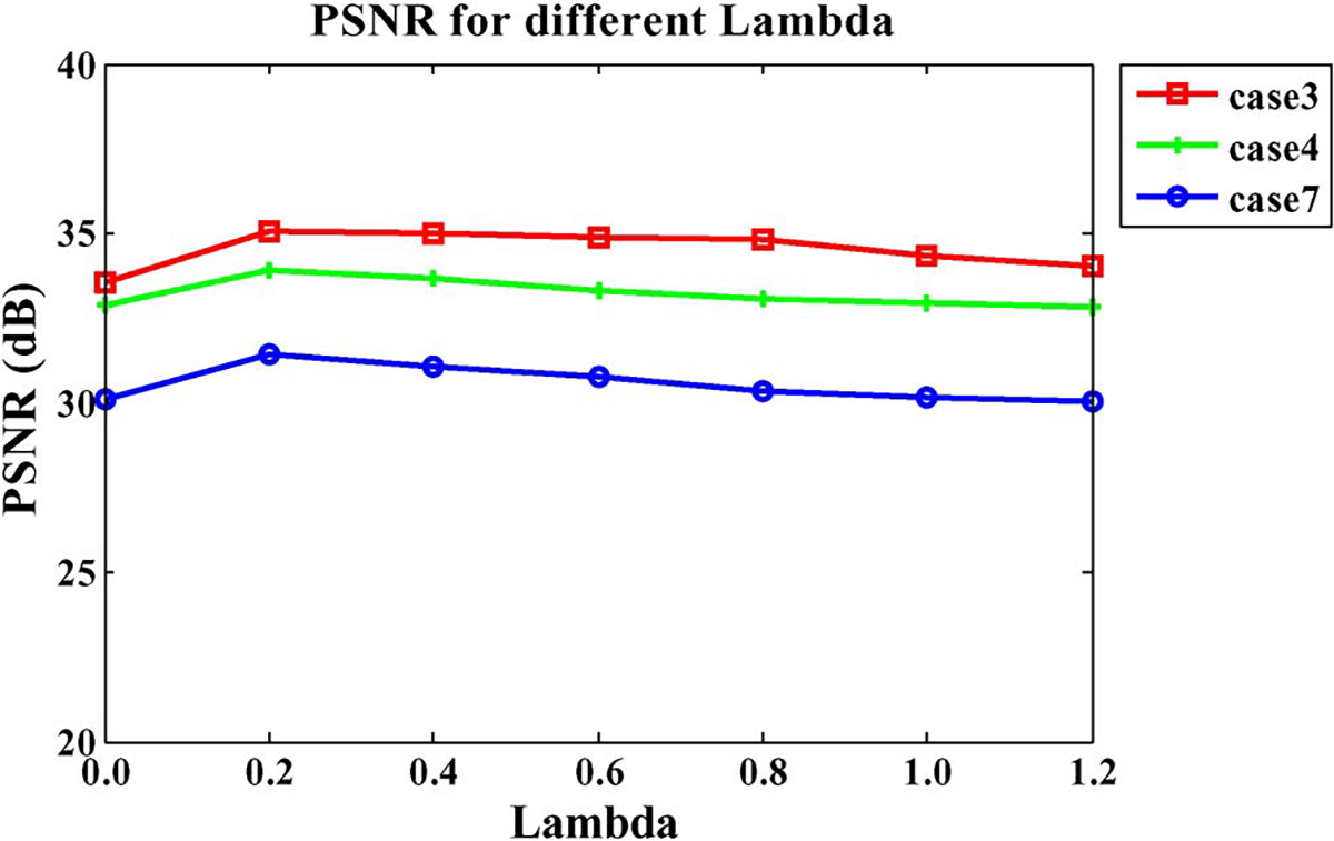
Influence of parameter .
Parameter :
Now we turn to , a tolerance factor for controlling the bias of selected patches towards the two consecutive patches. Similar to the analysis for parameter , we also select three cases to test the impact of . The PSNR values with different ranging from 1.1 to 2.3 are shown in Fig. 8. It is clear that for the low values (≤1.3), the higher PSNR values are achieved since the strict constraint is helpful to reject the unfit patches. We, therefore, set throughout all experiments presented in Sections III-C and III-D.
Fig. 8.
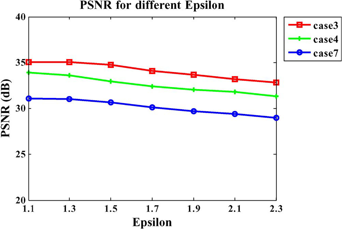
Influence of parameter .
Second Step: Hierarchical Patch-Based Sparse Representation:
We have mentioned previously that, in order to reduce blocking artifacts, the image patches are allowed to overlap as much as 2/3 of the patch size. This will however blur the reconstructed intermediate slices. To overcome this problem, we hierarchically decrease the patch size and overlap area, and repeatedly update the reconstructed slice to reduce image blurring.
| (7) |
Let denote the initial reconstructed image and denote a local patch of . We solve , where is the current estimated patch, subject to the following condition:
| (8) |
Note that this equation is similar to (5). The difference is that now we use the initial image as the constraint, instead of and . The dictionary is also adaptively built as described in Section II-C, and the solution is the same as described in Section II-D.
To ensure the consistency between iterations, we further propose a penalty function in the following form:
| (9) |
The first term is the fidelity term, where is the slice reconstructed in the previous iteration. The second term is the penalty term constraining the difference between the updated image and the current image , which is reconstructed using patches . The parameter controls the tradeoff between the two terms. This is actually a quadratic problem that has a closed-form solution
| (10) |
where is used to replace in the next iteration. We progressively reduce the patch size and pixel overlap and then perform the previous procedure iteratively to obtain the final result. The effectiveness of this hierarchical scheme is demonstrated in Figs. 10 and 11, which will be explained as follows. Also, further details are provided in Section III-C.
Fig. 10.
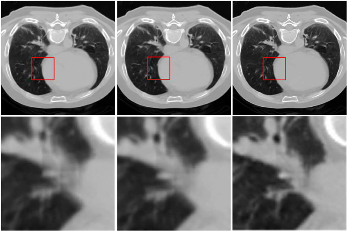
Hierarchical structural refinement. From left to right: reconstruction results from the first step via 32 × 32 patches with 24-pixel overlap, first iteration of the second step via 16 × 16 patches with 4-pixel overlap, and second iteration of the second step via 8 × 8 patches with 2-pixel overlap, respectively.
Fig. 11.
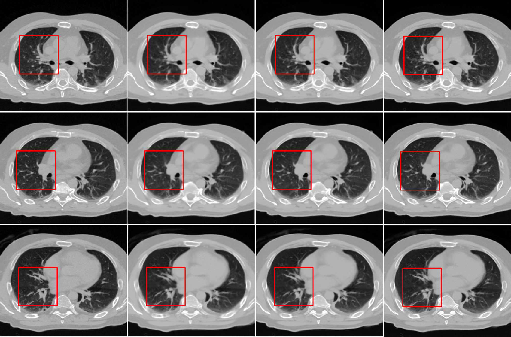
Results for three different slices reconstructed using hierarchical strategy. From left to right: ground truth and reconstructed images from the first step, first iteration of second step, and second iteration of the second step, respectively.
E. Method Summary
To summarize, two major steps are involved in our proposed intermediate slice reconstruction algorithm. The first step is the reconstruction of initial slices based on neighborhood constraints. The second step is the hierarchical refinement of the initial results. A step-by-step summary of this fully automatic algorithm is given as follows.
Input: 4D-CT images with all phases.
- First step: Reconstruct the initial intermediate slice.
- For a patch of a particular size of , perform a raster-scan with overlap in each direction.
- Build adaptive dictionary for .
- Solve the optimization problem defined in (6) with and as constraints, then output the result .
- Assemble the output into image as output.
- Second step: Iterative refinement—perform the following steps for each iteration.
Output: Output as the final result .
Go through all the intermediate slices by repeating Steps 2–4 to obtain the final resolution-enhanced 4D-CT lung data.
III. Results
A. Data and Preprocessing
Evaluation of the proposed method was performed based on a publicly available dataset that was provided by the DIR-lab [41]. The dataset consists of ten cases of 4D-CT. Each case was acquired at 2.5 mm slice spacing in ten phases, employing a General Electric Discovery DT PET/CT scanner. The 4D-CT images covered the entire thorax and upper abdomen. For case1 to case5, the in-plane grid size is 256 × 256, and the in-plane voxel dimensions range from (0.97 × 0.97) to (1.16 × 1.16) mm2. For case6 to case10, the in-plane grid size is 512 × 512, and the in-plane voxel dimensions are all (0.97 × 0.97) mm2. Detailed information regarding the dataset is shown in Table III.
TABLE III.
Imaging Parameters Associated With Each of Ten Cases Used for Evaluation
| Original Data Set | In-plane Grid Size | In-plane Dimensions (mm) | No. of Slices | Phase Number | Slice Spacing (mm) |
|---|---|---|---|---|---|
|
| |||||
| Case1 | 256 × 256 | 0.97 × 0.97 | 94 | 10 | 2.5 |
| Case2 | 256 × 256 | 1.16 × 1.16 | 112 | 10 | 2.5 |
| Case3 | 256 × 256 | 1.15 × 1.15 | 104 | 10 | 2.5 |
| Case4 | 256 × 256 | 1.13 × 1.13 | 99 | 10 | 2.5 |
| Case5 | 256 × 256 | 1.10 × 1.10 | 106 | 10 | 2.5 |
| Case6 | 512 × 512 | 0.97 × 0.97 | 128 | 10 | 2.5 |
| Case7 | 512 × 512 | 0.97 × 0.97 | 136 | 10 | 2.5 |
| Case8 | 512 × 512 | 0.97 × 0.97 | 128 | 10 | 2.5 |
| Case9 | 512 × 512 | 0.97 × 0.97 | 128 | 10 | 2.5 |
| Case 10 | 512 × 512 | 0.97 × 0.97 | 120 | 10 | 2.5 |
Images with dimensions 512 × 512 are cropped to 320 × 224 to reduce computational cost. To do this, for all the cases, we first segment each phase image into bone, soft tissue (muscle and fat), and lung [42]. The lung regions are used as the mask to extract the lung, as shown in Fig. 9. Quantitative evaluation will be all focused on the lung regions only.
Fig. 9.

From left to right: original image, mask for the lung, and extracted lung.
B. Experiment Settings
We simulate the 4D-CT with 5-mm slice thickness by removing every other slice from the data with 2.5-mm slice thickness. This gives us the ground truth to evaluate the effectiveness of our method in increasing the resolution from 5 to 2.5 mm. The algorithm was implemented using C++ and all the following evaluations are performed using a computer with a 2.4 GHz processor and 3 GB of memory.
Throughout the experiments, in the first step, we reconstruct initial images using a 32 × 32 patch size with a 24-pixel overlap. Then, in the second step, we hierarchically reduce the patch size and overlap pixels using two iterations. Specifically, we used a patch size of 16 × 16 with a 4-pixel overlap for the first iteration and 8 8 with 2-pixel overlap for the second iteration. As mentioned previously, parameter is set to 1.1, and parameter is set to 0.2, while parameter is set to 0.2, which will be explained as follows. Both visual and quantitative results are provided to demonstrate the performance of our proposed method. Linear and cubic-spline interpolation methods are also used as comparison methods.
C. Visual Inspection
Performance of Hierarchical Approach:
Fig. 10 shows an example of how the reconstructed image is progressively refined using the proposed hierarchical strategy. From left to right, results for decreasing patch sizes are shown. The enlarged views of the area marked by red squares are shown in the second row for better visual comparison. It is clear that the image becomes increasingly clearer in each step. Results for three different reconstructed slices are also shown in Fig. 11, where we can observe a similar progression to sharpness in these images. We note that is an important parameter for controlling the variation between images of two consecutive iterations. For a large , the penalty term in (9) will have a greater influence on the final estimation, and vice versa. We tested several values for this parameter and found that gave the best results both qualitatively and quantitatively. Thus, was selected for all experiments in this paper.
Comparison of Color-Coded Difference Maps:
For each of the three cases shown in Fig. 12, the ground truth is shown in the left column. The results given by linear interpolation, cubic spline interpolation, and the proposed method are shown in the second, third, and fourth columns, respectively. The color-coded difference maps computed with respect to the ground truth are also shown to aid comparison. It is apparent that our proposed method outperforms the conventional interpolation methods, which often cause undesirable artifacts. The proposed method makes principled use of information gathered from all other phase images to make up for the missing information and hence expectedly yields better results.
Fig. 12.
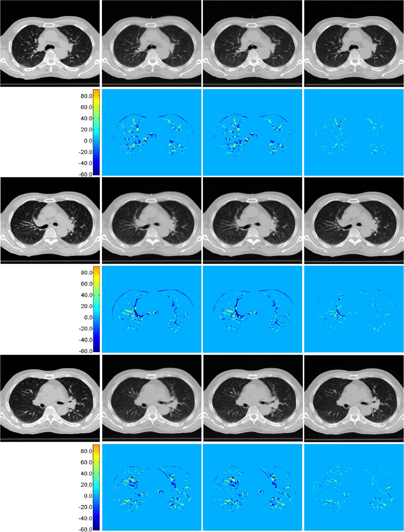
Reconstruction results and their difference maps. Results given by linear interpolation, cubic-spline interpolation, and proposed method are shown in the second, third, and fourth columns, respectively. Their color-coded difference maps compared to the ground truth (first column) are shown in the bottom of each panel.
Different views:
Fig. 13 shows typical axial, sagittal, and coronal views of another case by our proposed method. These results again show the best performance achieved by the proposed method. The corresponding difference maps in Fig. 14 and the enlarged views in Fig. 15 further confirm the best performance by our proposed method. In Fig. 15, regions in the red boxes are enlarged in the fourth, fifth and sixth rows, respectively. It can be observed that our method yields results with greater vessel continuity.
Fig. 13.
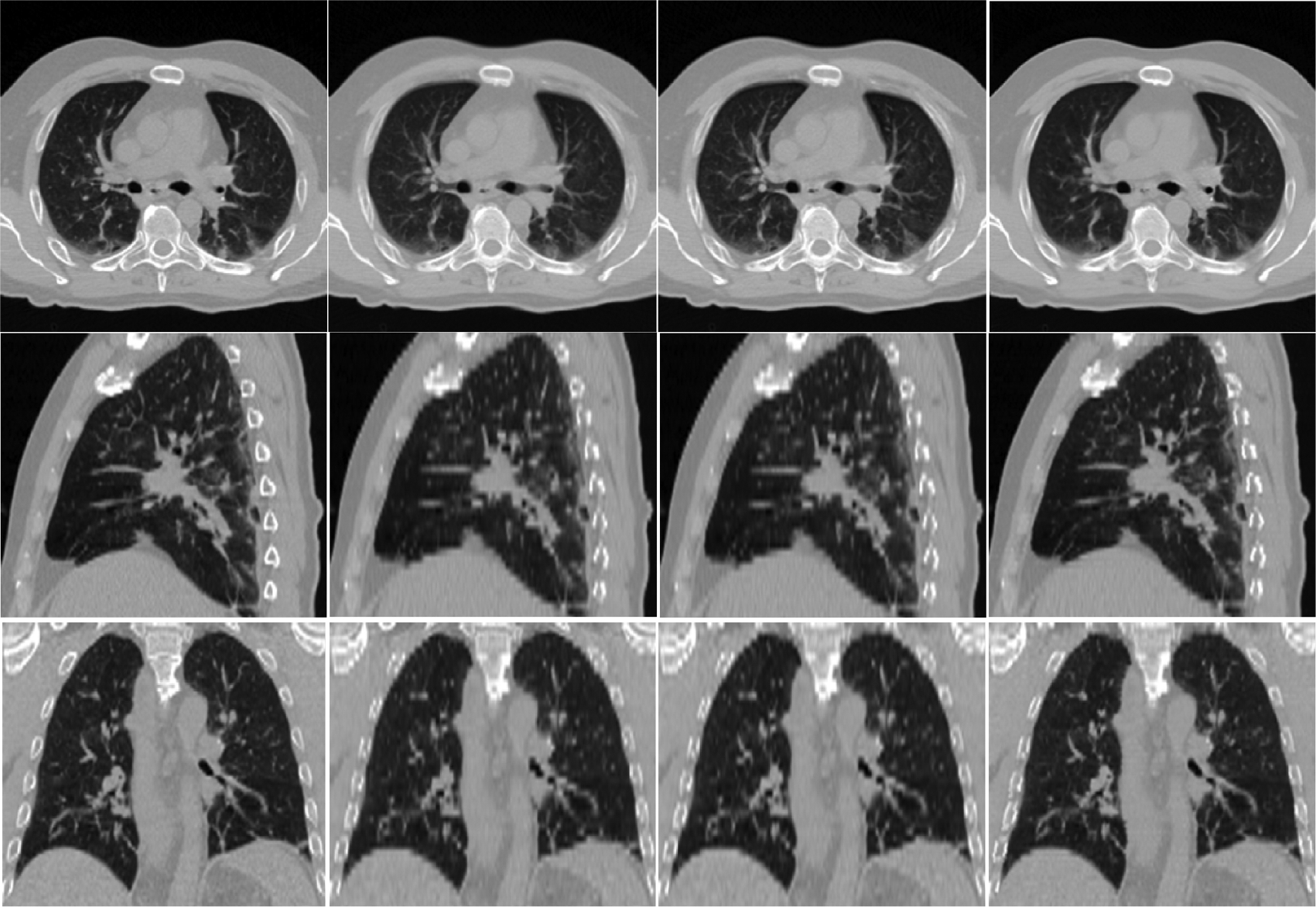
Axial, sagittal and coronal views of the resolution-enhanced images. From left to right: ground truth, and results given by linear interpolation, cubic-spline interpolation, and our method.
Fig. 14.
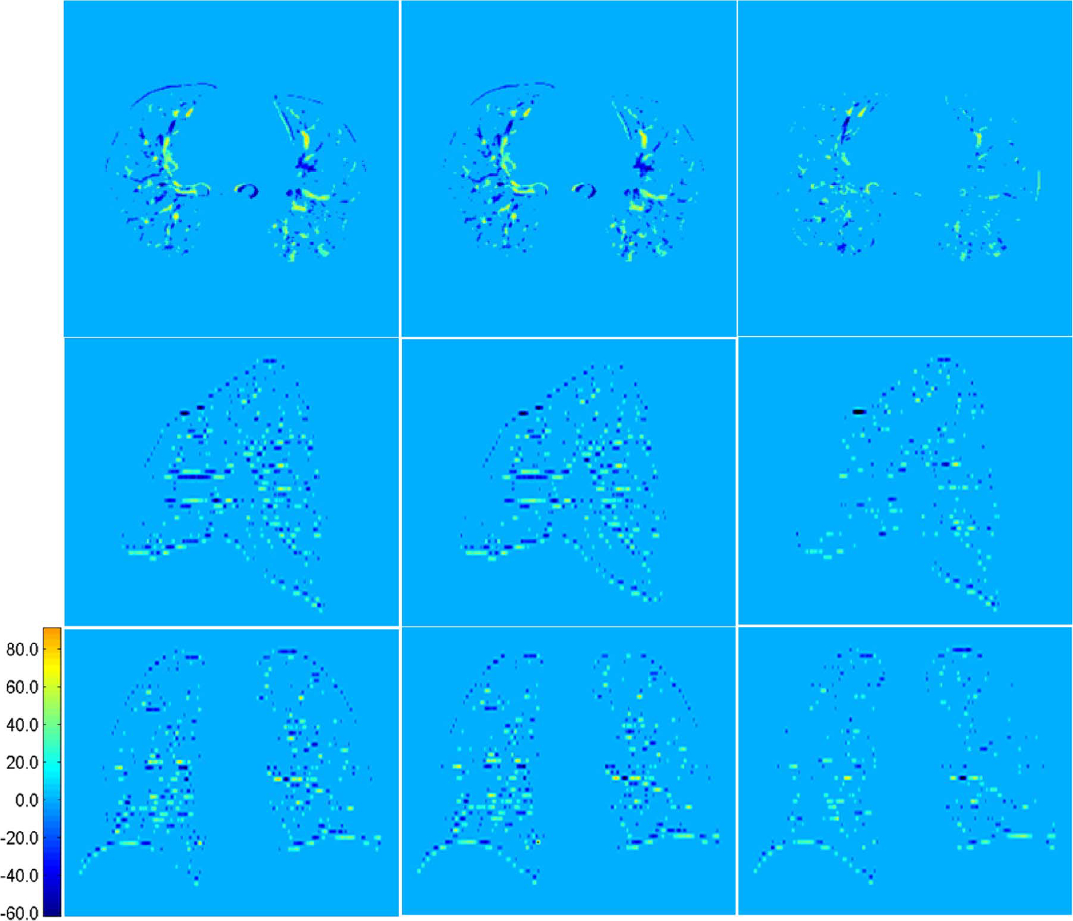
Axial, sagittal and coronal views of difference maps for results shown in Fig. 13. From left to right are the difference maps computed based on results given by linear interpolation, cubic-spline interpolation, and our method, respectively.
Fig. 15.
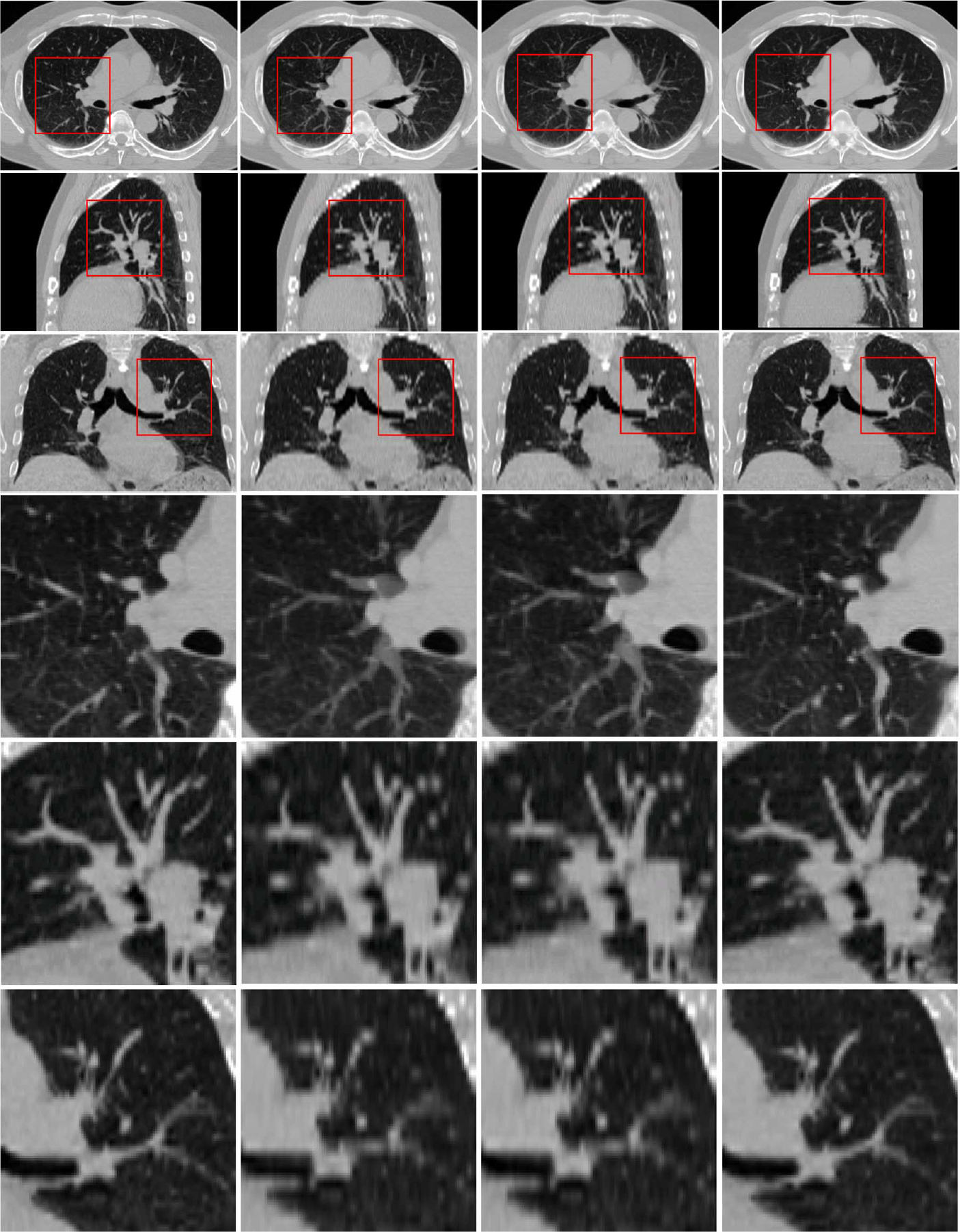
Enlarged views. Ground truth data is displayed on the left column. Results given by linear interpolation, cubic-spline interpolation, and our method are shown in second, third, fourth columns, respectively. Areas in red box are enlarged and shown in fourth, fifth, and sixth rows, respectively.
Pathological case:
Fig. 16 shows the reconstruction results in a slice with tumor. As demonstrated in the figure, both linear and cubic-spline interpolation yield tumors that are larger in size than the ground truth. This result will potentially increase risk of hurting normal tissue during radiotherapy. On the other hand, the proposed method is capable of reconstructing the tumor with greater accuracy, hence potentially better for protecting normal tissues and treating lung tumors during radiotherapy.
Fig. 16.
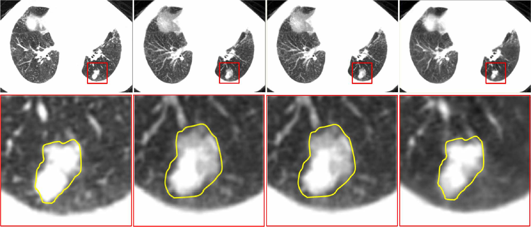
Results for a pathological case. Ground truth data is displayed on the left column. Results given by linear interpolation, cubic-spline interpolation, and our method are shown in second, third, and fourth columns, respectively. Tumor area in red box is enlarged and shown in the second row.
D. Quantitative Comparison With Other Interpolation Methods
Two quality measures were employed for the purpose of evaluation. The first is the peak signal-to-noise ratio (PSNR), which is widely used in signal and image processing to measure reconstruction error. The other is the structural similarity (SSIM) index [43], which is a metric that is motivated by the human visual system. PSNR is defined as the ratio between the maximum intensity value of the ground truth image and the power of corrupting noise (the average sum of squared differences between the ground truth and reconstructed images). PSNR values are expressed in the logarithmic decibel scale. SSIM calculation is based on the average, variance, and covariance of intensity values between the ground truth and the reconstructed images. Average PSNR and SSIM values for each 4D-CT case are reported in Table IV. It is clear that our method achieves the highest PSNR values (typically 2 ~ 3 dB higher) and also the highest SSIM values for all cases.
TABLE IV.
Average PSNR (Top) and SSIM (Bottom) Values Obtained by Linear Interpolation, Cubic Spline Interpolation, and Proposed Method in All Ten Cases
| Case | Linear interpolation | Cubic-spline interpolation | Proposed method |
|---|---|---|---|
|
| |||
| Case 1 | 29.92 | 30.02 | 33.01 |
| 0.8972 | 0.8968 | 0.9358 | |
| Case 2 | 30.02 | 30.22 | 33.25 |
| 0.8888 | 0.8884 | 0.9278 | |
| Case 3 | 30.81 | 31.05 | 34.55 |
| 0.9126 | 0.9133 | 0.9478 | |
| Case 4 | 29.62 | 29.78 | 32.67 |
| 0.9184 | 0.9194 | 0.9486 | |
| Case 5 | 29.85 | 29.91 | 32.52 |
| 0.9060 | 0.9052 | 0.9376 | |
|
| |||
| Case 6 | 28.60 | 28.57 | 30.72 |
| 0.8788 | 0.8786 | 0.9151 | |
| Case 7 | 27.40 | 27.51 | 30.78 |
| 0.8412 | 0.8417 | 0.9014 | |
| Case 8 | 27.17 | 27.23 | 29.42 |
| 0.7924 | 0.7819 | 0.8475 | |
| Case 9 | 29.08 | 29.28 | 32.22 |
| 0.9119 | 0.9129 | 0.9404 | |
| Case 10 | 27.72 | 27.81 | 30.13 |
| 0.8508 | 0.8520 | 0.8999 | |
IV. Discussion and Conclusion
The resolution enhancement technology can be used to overcome the resolution limitations caused by constraints such as acquisition time and radiation dose. In this paper, we have proposed a novel patch-based resolution enhancement method to improve the superior–inferior resolution of lung 4D-CT. We take advantage of complementary image information across all phases to recover the missing structural information in the intermediate slides of each phase. This is particularly achieved by using a hierarchical patch-based sparse representation approach with locally adaptive patch dictionaries. The key advantages of our work can be summarized as follows: 1) capable of integrating complementary information from different phases for reconstructing high-resolution 4D-CT data; 2) fully automatic and data-driven; 3) requires only data from each patient; and 4) requires no construction of a global dictionary. All these are the attractive properties that will also benefit the resolution enhancement of other 4-D imaging data (e.g., 4-D cardiac ultrasonic data).
An alternative approach for resolution enhancement is registration-based interpolation [17]. This approach, however, is not effective for the current application. The main reason is that the performance of registration-based interpolation approaches relies heavily on the accurate anatomical alignment. However, due to low-resolution of the lung 4D-CT data along the inferior–superior direction, the structural shapes vary rapidly and could be significantly different across even the neighboring slices. This poses a challenge to the registration-based interpolation approaches. Fig. 17 shows the example results for registration between two neighboring lung CT slices using a B-spline-based registration method [44]. It can be observed that accurate registration cannot be satisfactorily achieved within the lung area, since structures are vastly dissimilar between consecutive slices.
Fig. 17.
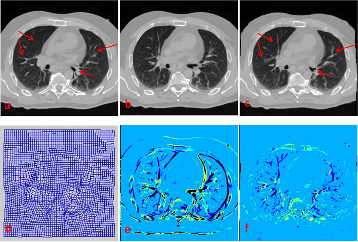
Registration of consecutive slices based on Myronenko and Song’s method [44]. (a) and (b) Consecutive slices, with (a) taken as target image and (b) as source image. (c) Warped source image, generated using deformation field shown in (d). (e) Difference map between (a) and (b). (f) Difference map between (a) and (c). Registration is very inaccurate within the lung area [compare (a) and (c), as well as (e) and (f)] due to large inter-slice structural differences.
We have demonstrated that the hierarchical scheme improves reconstruction results significantly. Since the initial estimate provides only a coarse estimation of the structures with the use of relatively larger-scale patches, the estimation at this scale is predominantly driven by large-scale structures, where smaller scale structures are neglected. Thus, in the second step, the hierarchical approach is necessary to refine the details of small-scale structures and at the same time reduce imaging artifacts, as discussed in Section III-C.
In our current implementation, we partition the intermediate slice into same-sized patches at each iteration. This does not take into account the fact that anatomical structures are manifested in different scales. In the future, we will extend the current framework by dividing the slice into structurally adaptive patches, i.e., using a quadtree-based strategy [52], for adaptive reconstruction of intermediate slices.
Patch estimates are currently combined by simple averaging, mainly to reduce computational time. Since reconstruction is performed in a hierarchical fashion from large patches to small patches, blocking artifacts that normally result from simple averaging could be minimized. But, more elaborate means of patch aggregation are expected to further improve the reconstruction results.
The current framework can be further improved by incorporating better distance constraints in (1), such as manifold motivated metrics [40], [45], [46]. Actually, a manifold-based interpolation method has been proven more effective for interpolation of heart MR data [47]. Also, the choice of image features will influence the final reconstruction results. In this work, we have simply utilized gradient features as popularly used in super-resolution reconstruction of natural images [33], [48] for guiding patch representation. In the future work, we will investigate how the proposed approach can be improved by using other features, such as the features derived from Haar wavelets [49], histograms of gradients (HOG) [50], and local binary patterns (LBP) [51].
In summary, we have presented in this paper a novel technique for enhancing the superior–inferior resolution of 4D-CT. Evaluation based on 4D-CT data from a public dataset indicates that the proposed method consistently outperforms the conventional interpolation-based approaches, for both normal and pathological cases. Our future work will be directed to further improvement of the propose method as outlined above, as well as the evaluation of feasibility of applying our method to facilitate accurate dose planning in radiation therapy.
Acknowledgments
This work was supported in part by the Major State Basic Research Development Program of China under Grant 2010CB732500, in part by the National Natural Science Foundation of China under Grant 31271067, in part by the Science and Technology Planning Project of Guangzhou under Grant 2010J-E471, and in part by the National Institutes of Health under Grant CA140413.
Appendix
Given , the optimization of weighting vector in (7) consists of three steps.
Calculate the correlation matrix , with defined as the inner production of and is the inverse of matrix .
If the constraints is fitted on (7), compute the Lagrange multiplier , where , and denotes the transpose.
The weight for reconstruction is computed as .
Contributor Information
Yu Zhang, Department of Radiology and Biomedical Research Imaging Center (BRIC), University of North Carolina, Chapel Hill, NC 27599 USA; School of Biomedical Engineering, Southern Medical University, Guangzhou 510515, China.
Guorong Wu, Department of Radiology and Biomedical Research Imaging Center (BRIC), University of North Carolina, Chapel Hill, NC 27599 USA.
Pew-Thian Yap, Department of Radiology and Biomedical Research Imaging Center (BRIC), University of North Carolina, Chapel Hill, NC 27599 USA.
Qianjin Feng, School of Biomedical Engineering, Southern Medical University, Guangzhou 510515, China.
Jun Lian, Department of Radiation Oncology, University of North Carolina, Chapel Hill, NC 27599 USA.
Wufan Chen, School of Biomedical Engineering, Southern Medical University, Guangzhou 510515, China.
Dinggang Shen, Department of Radiology and Biomedical Research Imaging Center (BRIC), University of North Carolina, Chapel Hill, NC 27599 USA.
References
- [1].Keall P, Mageras G, Balter J, Emery R, Forster K, Jiang S, Kapatoes J, Low D, Murphy M, Murray B, Ramsey C, Van Herk M, Vedam S, Wong J, and Yorke E, “The management of respiratory motion in radiation oncology report of AAPM Task Group 76,” Med. Phys, vol. 33, no. 10, pp. 3874–3900, Sep. 2006. [DOI] [PubMed] [Google Scholar]
- [2].Zhang X, Zhao K-L, Guerrero TM, McGuire SE, Yaremko B, Komaki R, Cox JD, Hui Z, Li Y, Newhauser WD, Mohan R, and Liao Z, “4D CT-based treatment planning for intensity-modulated radiation therapy and proton therapy for distal esophagus cancer,” Int. J. Radiat. Oncology., Biol., Phys, vol. 72, no. 1, pp. 278–287, Sep. 2008. [DOI] [PMC free article] [PubMed] [Google Scholar]
- [3].Li R, Lewis JH, Cerviño LI, and Jiang SB, “4D CT sorting based on patient internal anatomy,” Phys. Med. Biol, vol. 54, no. 15, pp. 4821–4833, August 2009. [DOI] [PubMed] [Google Scholar]
- [4].Georg M, Souvenir R, Hope A, and Pless R, “Manifold learning for 4D CT reconstruction of the lung,” in Proc. IEEE Comput. Soc. Conf. Comput. Vis. Pattern Recognit. Workshops, Jun. 2008, pp. 1–8. [Google Scholar]
- [5].Khan F, Bell G, Antony J, Palmer M, Balter P, Bucci K, and Chapman MJ, “The use of 4DCT to reduce lung dose: A dosimetric analysis,” Med. Dosimetry, vol. 34, no. 4, pp. 273–278, Winter, 2009. [DOI] [PubMed] [Google Scholar]
- [6].Li T, Schreibmann E, Thorndyke B, Tillman G, Boyer A, Koong A, Goodman K, and Xing L, “Radiation dose reduction in four-dimensional computed tomography,” Med. Phys, vol. 32, no. 12, pp. 3650–3660, Dec. 2005. [DOI] [PubMed] [Google Scholar]
- [7].Werner R, Ehrhardt J, Frenzel T, Säring1 D, Lu W, Low D, and Handels H, “Motion artifact reducing reconstruction of 4D CT image data for the analysis of respiratory dynamics,” Methods Inform. Med, vol. 46, no. 3, pp. 254–260, Mar. 2007. [DOI] [PubMed] [Google Scholar]
- [8].Ehrhardt J, Werner R, Säring D, Frenzel T, Lu W, Low D, and Handels H, “An optical flow based method for improved reconstruction of 4D CT data sets acquired during free breathing,” Med. Phys, vol. 34, no. 2, pp. 711–721, Feb. 2007. [DOI] [PubMed] [Google Scholar]
- [9].Tian Z, Jia X, Dong B, and Jiang SB, “Low-dose 4DCT reconstruction via temporal nonlocal means,” Med. Phys, vol. 38, no. 3, pp. 1359–1365, Mar. 2011. [DOI] [PubMed] [Google Scholar]
- [10].Schreibmann E, Chen GTY, and Xing L, “Image interpolation in 4D CT using a BSpline deformable registration model,” Int. J. Radiat. Oncol., Biol., Phys, vol. 64, no. 5, pp. 1537–1550, Apr. 2006. [DOI] [PubMed] [Google Scholar]
- [11].Sarruta D, Boldea V, Miguet S, and Ginestet C, “Simulation of four-dimensional CT images from deformable registration between inhale and exhale breath-hold CT scans,” Med. Phys, vol. 33, no. 3, p. 17, March 2006. [DOI] [PubMed] [Google Scholar]
- [12].Grevera GJ and Udupa JK, “An objective comparison of 3-D image interpolation methods,” IEEE Trans. Med. Imag, vol. 17, no. 4, pp. 642–652, Aug. 1998. [DOI] [PubMed] [Google Scholar]
- [13].Frakes DH, Dasi LP, Pekkan K, Kitajima HD, Sundareswaran K, Yoganathan AP, and Smith MJT, “A new method for registration-based medical image interpolation,” IEEE Trans. Med. Imag, vol. 27, no. 3, pp. 370–377, Mar. 2008. [DOI] [PubMed] [Google Scholar]
- [14].Tong-Yee L and Wen-Hsiu W, “Morphology-based three-dimensional interpolation,” IEEE Trans. Med. Imag, vol. 19, no. 7, pp. 711–721, Jul. 2000. [DOI] [PubMed] [Google Scholar]
- [15].Williams WL and Barrett WA, “Optical flow interpolation of serial slice images,” in Proc. SPIE Med. Imag, Feb. 1993, pp. 93–104. [Google Scholar]
- [16].Frakes DH, Conrad CP, Healy TM, Monaco JW, Fogel M, Sharma S, Smith MJT, and Yoganathan AP, “Application of an adaptive control grid interpolation technique to morphological vascular reconstruction,” IEEE Trans. Biomed. Eng, vol. 50, no. 2, pp. 197–206, Feb. 2003. [DOI] [PubMed] [Google Scholar]
- [17].Penney GP, Schnabel JA, Rueckert D, Viergever MA, and Niessen WJ, “Registration-based interpolation,” IEEE Trans. Med. Imag, vol. 23, no. 7, pp. 922–926, Jul. 2004. [DOI] [PubMed] [Google Scholar]
- [18].Bose NK and Boo KJ, “High-resolution image reconstruction with multisensors,” Int. J. Imag. Syst. Technol, vol. 9, no. 4, pp. 294–304, Dec. 1998. [Google Scholar]
- [19].Greenspan H, “Super-resolution in medical imaging,” Comput. J, vol. 52, no. 1, pp. 43–63, January 2009. [Google Scholar]
- [20].Rousseau F, “A non-local approach for image super-resolution using intermodality priors,” Med. Image Anal, vol. 14, no. 4, pp. 594–605, May 2010. [DOI] [PMC free article] [PubMed] [Google Scholar]
- [21].Greenspan H, Oz G, Kiryati N, and Peled S, “MRI inter-slice reconstruction using super-resolution,” Magn. Resonance Imag, vol. 20, no. 5, pp. 437–446, Jun. 2002. [DOI] [PubMed] [Google Scholar]
- [22].Rousseau F, Glenn OA, Iordanova B, Rodriguez-Carranza C, Vigneron DB, Barkovich JA, and Studholme C, “Registration-based approach for reconstruction of high-resolution in Utero Fetal MR brain images,” Acad. Radiol, vol. 13, no. 9, pp. 1072–1081, Sep. 2006. [DOI] [PubMed] [Google Scholar]
- [23].Gholipour A, Estroff JA, and Warfield SK, “Robust super-resolution volume reconstruction from slice acquisitions: Application to fetal brain MRI,” IEEE Trans. Med. Imag, vol. 29, no. 10, pp. 1739–1758, Oct. 2010. [DOI] [PMC free article] [PubMed] [Google Scholar]
- [24].Joshi SH, Marquina A, Osher SJ, Dinov I, Van Horn JD, and Toga AW, “MRI resolution enhancement using total variation regularization,” in Proc. IEEE Int. Symp. Biomed. Imag.: From Nano to Macro, Jun. 2009, pp. 161–164. [DOI] [PMC free article] [PubMed] [Google Scholar]
- [25].Irani M and Peleg S, “Motion analysis for image enhancement: Resolution, occlusion, and transparency,” J. Visual Commun. Image Representat, vol. 4, no. 4, pp. 324–335, Dec. 1993. [Google Scholar]
- [26].Wallach D, Lamare F, Kontaxakis G, and Visvikis D, “Super-resolution in respiratory synchronized positron emission tomography,” IEEE Trans. Med. Imag, vol. 31, no. 2, pp. 438–448, Feb. 2012. [DOI] [PubMed] [Google Scholar]
- [27].Zhang Y, Wu G, Yap P-T, Feng Q, Lian J, Chen W, and Shen D, “Reconstruction of super-resolution lung 4D-CT using a patch-based sparse representation,” in Proc. IEEE Conf. Comput. Vis. Pattern Recognit., Providence, RI, Jun. 2012. [Google Scholar]
- [28].Elad M and Aharon M, “Image denoising via sparse and redundant representations over learned dictionaries,” IEEE Trans. Image Process, vol. 15, no. 12, pp. 3736–3745, Dec. 2006. [DOI] [PubMed] [Google Scholar]
- [29].Mairal J, Elad M, and Sapiro G, “Sparse representation for color image restoration,” IEEE Trans. Image Process, vol. 17, no. 1, pp. 53–69, Jan. 2008. [DOI] [PubMed] [Google Scholar]
- [30].Fadili MJ, Starck J-L, and Murtagh F, “Inpainting and zooming using sparse representations,” Comput. J, vol. 52, no. 1, pp. 64–79, Jan. 2009. [Google Scholar]
- [31].Mairal J, Bach F, Ponce J, Sapiro G, and Zisserman A, “Discriminative learned dictionaries for local image analysis,” in Proc. IEEE Conf. Comput. Vis. Pattern Recognit, Jun. 2008, pp. 1–8. [Google Scholar]
- [32].Winn J, Criminisi A, and Minka T, “Object categorization by learned universal visual dictionary,” in Proc. 10th IEEE Int. Conf. Comput. Vis, Oct. 2005, pp. 1800–1807. [Google Scholar]
- [33].Jianchao Y, Wright J, Huang TS, and Yi M, “Image super-resolution via sparse representation,” IEEE Trans. Image Process, vol. 19, no. 11, pp. 2861–2873, Nov. 2010. [DOI] [PubMed] [Google Scholar]
- [34].Ivana T, Ivana J, Frossard P, Vetterli M, and Duric N, “Ultrasound tomography with learned dictionaries,” in Proc. IEEE Int. Conf. Acoustics Speech Signal Process, Mar. 2010, pp. 5502–5505. [Google Scholar]
- [35].Chen Y and Ye X, “A novel method and fast algorithm for MR image reconstruction with significantly under-sampled data,” Inverse Problems Imag, vol. 4, no. 2, pp. 223–240, 2010. [Google Scholar]
- [36].Ravishankar S and Bresler Y, “MR image reconstruction from highly undersampled k-Space data by dictionary learning,” IEEE Trans. Med. Imag, vol. 30, no. 5, pp. 1028–1041, May 2011. [DOI] [PubMed] [Google Scholar]
- [37].Aharon M, Elad M, and Bruckstein A, “K-SVD: An algorithm for designing overcomplete dictionaries for sparse representation,” IEEE Trans. Signal Process, vol. 54, no. 11, pp. 4311–4322, Nov. 2006. [Google Scholar]
- [38].Davis G, Mallat S, and Avellaneda M, “Adaptive greedy approximations,” Constructive Approx, vol. 13, no. 1, pp. 57–98, Mar. 1997. [Google Scholar]
- [39].Xu Z and Sun J, “Image inpainting by patch propagation using patch sparsity,” IEEE Trans. Image Process, vol. 19, no. 5, pp. 1153–1165, May 2010. [DOI] [PubMed] [Google Scholar]
- [40].Roweis ST and Saul LK, “Nonlinear dimensionality reduction by locally linear embedding,” Science, vol. 290, no. 5500, pp. 2323–2326, Dec. 2000. [DOI] [PubMed] [Google Scholar]
- [41].Castillo R, Castillo E, Guerra R, Johnson VE, McPhail T, Garg AK, and Guerrero T, “A framework for evaluation of deformable image registration spatial accuracy using large landmark point sets,” Phys. Med. Biol, vol. 54, no. 7, pp. 1849–1870, Apr. 2009. [DOI] [PubMed] [Google Scholar]
- [42].Hu S, Hoffman EA, and Reinhardt JM, “Automatic lung segmentation for accurate quantitation of volumetric X-ray CT images,” IEEE Trans. Med. Imag, vol. 20, no. 6, pp. 490–498, Jun. 2001. [DOI] [PubMed] [Google Scholar]
- [43].Zhou W, Bovik AC, Sheikh HR, and Simoncelli EP, “Image quality assessment: From error visibility to structural similarity,” IEEE Trans. Image Process, vol. 13, no. 4, pp. 600–612, Apr. 2004. [DOI] [PubMed] [Google Scholar]
- [44].Myronenko A and Song X, “Intensity-based image registration by minimizing residual complexity,” IEEE Trans. Med. Imag, vol. 29, no. 11, pp. 1882–1891, Nov. 2010. [DOI] [PubMed] [Google Scholar]
- [45].Bregler C and Omohundro SM, “Nonlinear manifold learning for visual speech recognition,” in Proc. 5th Int. Conf. Comput. Vis, Jun. 1995, pp. 494–499. [Google Scholar]
- [46].Tenenbaum JB, Silva VD, and Langford JC, “A global geometric framework for nonlinear dimensionality reduction,” Science, vol. 290, no. 5500, pp. 2319–2323, Dec. 2000. [DOI] [PubMed] [Google Scholar]
- [47].Souvenir R, Qilong Z, and Pless R, “Image manifold interpolation using free-form deformations,” in Proc. IEEE Int. Conf. Image Process, Oct. 2006, pp. 1437–1440. [Google Scholar]
- [48].Hong C, Dit-Yan Y, and Yimin X, “Super-resolution through neighbor embedding,” in Proc. IEEE Conf. Comput. Vis. Pattern Recognit, Jun. 2004, pp. 275–282. [Google Scholar]
- [49].Mallat SG, “A theory for multiresolution signal decomposition: The wavelet representation,” IEEE Trans. Pattern Anal. Mach. Intell, vol. 11, no. 7, pp. 674–693, Jul. 1989. [Google Scholar]
- [50].Dalal N and Triggs B, “Histograms of oriented gradients for human detection,” in Proc. IEEE Comput. Soc. Conf. Comput. Vis. Pattern Recognit, Jun. 2005, pp. 886–893. [Google Scholar]
- [51].Ojala T, Pietikainen M, and Maenpaa T, “Multiresolution gray-scale and rotation invariant texture classification with local binary patterns,” IEEE Trans. Pattern Anal. Mach. Intell, vol. 24, no. 7, pp. 971–987, Jul. 2002. [Google Scholar]
- [52].Finkel RA and Bentley JL, “Quad trees a data structure for retrieval on composite keys,” Acta Informatica, vol. 4, no. 1, pp. 1–9, Mar. 1974. [Google Scholar]


