Abstract
Background:
Using multiple modalities of biomarkers, several machine leaning-based approaches have been proposed to characterize patterns of structural, functional and metabolic differences discernible from multimodal neuroimaging data for Alzheimer’s disease (AD). Current investigations report several studies using binary classification often augmented with local feature selection methods, while fewer other studies address the challenging problem of multiclass classification.
New Method:
To assess the merits of each of these research directions, this study introduces a supervised Gaussian discriminative component analysis (GDCA) algorithm, which can effectively delineate subtle changes of early mild cognitive impairment (EMCI) group in relation to the cognitively normal control (CN) group. Using 251 CN, 297 EMCI, 196 late MCI (LMCI), and 162 AD subjects from the Alzheimer’s Disease Neuroimaging Initiative (ADNI) and considering both structural and functional (metabolic) information from magnetic resonance imaging (MRI) and positron emission tomography (PET) modalities as input, the proposed method conducts a dimensionality reduction algorithm taking into consideration the interclass information to define an optimal eigenspace that maximizes the discriminability of selected eigenvectors.
Results:
The proposed algorithm achieves an accuracy of 79.25% for delineating EMCI from CN using 38.97% of Gaussian discriminative components (i.e., dimensionality reduction). Moreover, for detecting the different stages of AD, a multiclass classification experiment attained an overall accuracy of 67.69%, and more notably, discriminates MCI and AD groups from the CN group with an accuracy of 75.28% using 48.90% of the Gaussian discriminative components.
Comparison with existing method(s):
The classification results of the proposed GDCA method outperform the more recently published state-of-the-art methods in AD-related multiclass classification tasks, and seems to be the most stable and reliable in terms of relating the most relevant features to the optimal classification performance.
Conclusion:
The proposed GDCA model with its high prospects for multiclass classification has a high potential for deployment as a computer aided clinical diagnosis system for AD.
Keywords: Alzheimer’s disease, computer-aided diagnosis, dimensionality reduction, mild cognitive impairment (MCI), multiclass classification, multimodal analysis
Graphical Abstract
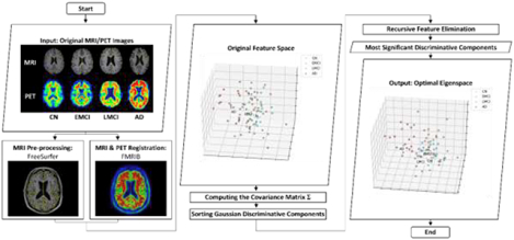
1. INTRODUCTION
In recent years, machine learning approaches have been applied in a growing number of studies to characterize patterns of structural, functional and metabolic difference discernible from multimodal neuroimaging data, such as magnetic resonance imaging (MRI) [1–6] and positron emission tomography (PET) [4–8]. The high-dimensionality nature of neuroimaging data often raises a necessity for dimensionality reduction and feature selection to obtain an optimal decision space. The results reported in some recent studies indicate that appropriate decision-making methods could improve the classification accuracy regardless of the sample size [9–12].
Voxel-based MRI studies have demonstrated that widely distributed cortical and subcortical brain regions show atrophy patterns in mild cognitive impairment (MCI), preceding the onset of Alzheimer’s disease (AD) [13–17]. A recent study has indicated the clinical utility of PET imaging for differential diagnosis in early onset dementia in support of clinical diagnosis of participants with AD and noncarrier APOE ε4 status who are older than 70 years [18]. Empirical evidence suggests that appropriate feature selection could preserve the complementary inter-modality information; therefore, the proposed dimensionality reduction model shows great potential for extracting relevant information from all modalities associated with the progression of AD. Currently, the Principal Component Analysis (PCA) model remains the most widely used method in dimensionality reduction and feature selection tasks [19, 20]. However, for machine learning tasks like classification and regression analyses, PCA is applied as an unsupervised method not considering the interclass information, such as data labels and target values; therefore, in many cases the consequently implemented feature selection methods may not be able to find the optimal decision spaces for the corresponding tasks. Moreover, the importance of PCA generated components is estimated by the variance, which are not often equivalent to the significance of those components in machine learning tasks.
This study aims to introduce a supervised dimensionality reduction algorithm to characterize the important Gaussian discriminative components with respect to the structural, functional or metabolic measurements as observed in the MRI-PET combination associated with different stages of AD, focusing on the prodromal stage of MCI [21, 22]. The stage of MCI is subdivided into two stages, early MCI (EMCI) and late MCI (LMCI), as defined in the Alzheimer’s disease Neuroimaging Initiative (ADNI) data. Since alleviation of specific symptoms is possible through therapeutic interventions for some patients in the early or middle stages of AD, effective diagnosis of EMCI from cognitively normal control (CN) group is essentially important for the planning of early treatment. However, instead of utilizing PCA computed variances to determine the significances of different components, the proposed Gaussian discriminative component analysis (GDCA) makes use of Gaussian discriminant analysis (GDA) classifiers to reveal the discriminability of different components in terms of each component’s performance obtained by a designate machine learning task. This process is shown to lead to stable, reliable and accurate dimensionality reduction in multimodal neuroimaging biomarkers for effective classification, enhanced diagnosis and the monitoring of disease progression.
2. MATERIALS
The information of the subjects used in this study and the MRI data preprocessing and MRI/PET registration procedure are presented in this section.
2.1. Participants and Clinical Data
The data used in conducting this study were collected from the ADNI database (adni.loni.usc.edu). The ADNI was launched in 2003 as a public-private partnership, led by Principal Investigator Michael W. Weiner, MD. The primary goal of ADNI has been to test whether serial MRI, PET, other biological markers, and clinical and neuropsychological assessment can be combined to predict and gauge the progression of AD.
A total of 906 subjects were considered for this study, which were categorized into groups of CN (251), EMCI (297), LMCI (196) and AD (162). All individuals underwent structural MRI and Florbetapir (F18-AV45) PET imaging, where the time gap between the two imaging modalities was less than 3 months. Details of MRI and AV45 PET data acquisition can be found on the ADNI website. Summary statistics and participants counts are listed in Table 1.
Table 1.
Participant Demographic and Clinical Information
| CN (n=251) | EMCI (n=297) | LMCI (n=196) | AD (n=162) | |
|---|---|---|---|---|
| F/M | 128/123 | 132/165 | 85/111 | 68/94 |
| Age_PETb | 75.5(6.5)a | 71.5(7.4) | 73.8(8.1) | 74.9(7.8) |
| Age_MRIb | 75.3(6.6) | 71.3(7.4) | 73.6(8.0) | 74.7(7.8) |
| Education | 16.43(2.6) | 15.99(2.7) | 16.31(2.7) | 15.76(2.7) |
| MMSEcd | 29.04(1.2) | 28.32(1.6) | 27.61(1.9) | 22.77(2.7) |
| RAVLT_immediatecd | 45.3(10.6) | 39.5(10.8) | 33.2(10.8) | 22.3(7.0) |
Values are represented as mean(sd), except gender (F for female, M for male), which are frequencies instead
Significant group differences (ANOVA for continuous and Chi-square test for categorical values, significance level is 0.05 by default)
Significant group differences (ANCOVA adjusted for Age_PET)
Significant differences for all between-group post-hoc tests (Tukey’s HSD test)
2.2. Image Processing
2.2.1. MRI Data Preprocessing
The FreeSurfer (Version 5.3.0) was firstly performed under Linux system (centos4_x86_64) to transform the original MRI to the standard MNI 305 space, yielding the image referred to as T1.mgz, which is used as the reference image in the registration procedure, followed by skull-striping, segmenting, and delineating cortical and subcortical regions with the corresponding image result termed as aparc+aseg.mgz. Derived from the images, the following three shape measures were then calculated as morphological features on each of the 68 FreeSurfer labeled cortical regions for both hemispheres (34 per hemisphere): 1) cortical thickness, 2) surface area, and 3) cortical volume. Since version 5.3 of FreeSurfer was available, we tested the same data with FreeSurfer 6.0 and found minimal differences ranging from 1 to 5% and showing no statistical differences in terms of standardized uptake value ratio measurements (SUVRs).
2.2.2. MRI and PET Registration
With 12 degrees of freedom (DOF) onto the postprocessed T1 image, the AV45 PET was linearly registered (using trilinear interpolation), so that the regional amyloid deposition and gray matter atrophy are compared directly (i.e., thickness for cortical regions [23–26]), using the FMRIB Software Library (FSL) [27]. Moreover, in order to gain as much information as possible from PET images, which have relatively low resolution, the original AV45 PET with skull was utilized in this step. This registration process introduced in a recent study [28] guaranteed that AV45 PET image had the same segmentation and parcellation as the MRI image. Combined with aparc+aseg.mgz images, the registered AV45 PET was inspected to obtain the mean standardized uptake values (SUV) for all 68 FreeSurfer labeled cortical regions. The SUV of the whole cerebellum, including 4 regions of interest (left/right cerebellum cortex and left/right white matter), was used as the reference region. Finally, regional SUVs of those 68 cortical regions were normalized by the SUV of the whole cerebellum to get the cortical-to-cerebellum SUVRs. Accordingly, overall there are 4 different types of neuroimaging features associated with each of the 68 cortical regions, yielding 272 (4×68) features for each subject in the dataset.
3. METHODS
After obtaining all needed features derived from raw multimodal neuroimaging data, as aforementioned, a 272-dimensional feature vector was generated for each subject in the data set. In this section, the proposed GDCA algorithm is presented for the effective dimensionality reduction and early diagnosis of AD. The standard PCA is applied to the original data to find the principal components. Then, the discriminability of each component is estimated by a one-dimensional GDA classifier, and consequently, all components are sorted in order of the corresponding classification performance. Finally, the recursive feature elimination (RFE) is employed to determine the optimal dimensionality reduction of the Gaussian discriminant components in the classification outcome. Fig. 1 demonstrates the flowchart of the proposed GDCA model.
Fig. 1.
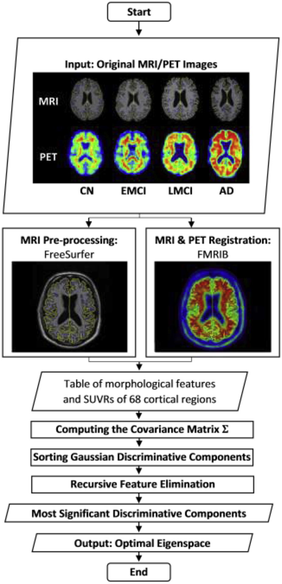
General flowchart of the proposed GDCA dimensionality reduction algorithm.
3.1. Gaussian Discriminative Component Analysis
3.1.1. Eigenvectors of the covariance matrix
The proposed classification problem can be formulated by having the machine learn to distinguish between CN (y = 0), EMCI (y = 1), LMCI (y = 2), and AD (y = 3), based on the extracted features . In order to determine the potential directions of Gaussian discriminative components of all features, the standard PCA method is carried out. Prior to running PCA, the data need to be normalized as follows:
| (1) |
where and are the mean vector and standard deviation vector of all data, respectively. This process zeros out the mean of the data, and rescales each feature to have unit variance, which ensures different features to have the same scale. After normalization, the covariance matrix Σ can then be computed utilizing the normalized data by the formula below:
| (2) |
where m is the total number of data points considered and is the transpose of the normalized data point . Then to project the original data into a k-dimensional subspace (k ≤ n), the eigenvector (j ≤ k) of the covariance matrix Σ can be computed to obtain the transformed features .
3.1.2. Supervised dimensionality reduction
As indicated earlier, the PCA model sorts the extracted eigenvectors (i.e., the direction of principal components) based on the variance represented by each eigenvector, without considering any information from the labels of data as an unsupervised algorithm. But, in general, only reducing the dimensionality to retain as much as possible of the variance cannot help in deciding the optimal subspace towards an optimal performance if a supervised machine learning scenario is contemplated. As a consequence, the proposed method capitalizes on a supervised dimensionality reduction model making use of a GDA-based classifier. Given the eigenvectors which were computed based on the covariance matrix Σ given in (2), the GDA model will be trained on each new feature in the transformed space to determine the discriminability of each component according to the corresponding classification performance, subsequently sorting the extracted principal components in order of their discriminability.
GDA can model p(x′|y), the distribution of the feature vector x′ in the transformed feature space given y ∈ {0,1,2,3}, assumed to be distributed according to a Gaussian distribution, with the generalized density function given in (3):
| (3) |
where is the mean vector in the new transformed feature space, Σ′ is the new covariance matrix, |Σ′| and Σ′−1 denote the determinant and inverse matrix of Σ′, respectively. To determine the discriminability of each component, since , the is the mean of the transformed feature, and Σ′ is the variance of the transformed feature. After modelling p(x′|y), Bayes rule is used to derive the posterior distribution on y given x′ as:
| (4) |
Here, p(y) denotes the class prior distribution, which cannot be determined when given a certain subject, so it is assumed to be absolutely random (for all a ≠ b, p(y = a) = p(y = b)). Furthermore, to make a prediction, it is not necessary to calculate p(x′), since
| (5) |
Therefore, for classification purposes, the following formula is used instead:
| (6) |
3.1.3. Recursive Component Elimination
The aforementioned classifier is applied to each component, so that for each eigenvector, the transformed features can be ranked in terms of classification outcome using cross validation. In this study, the classification accuracy is used as the key metric to measure performance, which means the discriminability of each component is determined by its corresponding classification accuracy expressed as follows:
| (7) |
which is the sum of True Positives (TP) and True Negatives (TN) divided by the sum of TP, False Positives (FP), TN, and False Negatives (FN).
Setting the computed accuracies as assigned weights to discriminative components, recursive feature elimination (RFE) is performed to select the optimal Gaussian discriminative components by recursively considering smaller and smaller sets of components. First, the entire set of components were applied to the classifier and estimated by the cross-validation performance. Then, the least important component is eliminated from current set of components. That procedure is recursively repeated on the pruned set until the desired set of Gaussian discriminative components is found with an optimal classification performance.
3.2. Classification Based on GDCA
From the proposed GDCA dimensionality reduction model, the optimal components are obtained in terms of the classification performance (i.e., the accuracy of that set of components selected), and would then be applied to other classification algorithms. Some other metrics are used as well, since, as a clinical application, the classification performance may not only be evaluated by the accuracy, but could also rely on precision, recall (or sensitivity) and specificity. The F1 score is also a widely used measure of performance in statistical analysis of binary classification, by which both precision and recall are taken into consideration. The formulas used to calculate these four metrics are expressed below:
| (8) |
| (9) |
| (10) |
| (11) |
In order to assess the ability of the obtained transformed feature space in performance improvement, several widely used classification algorithms are applied on the original feature space as well as the dimensionality reduced new feature space, including linear support vector machines (SVM), multilayer perceptron (MLP), and gradient boosting (GB) classifiers. To demonstrate the advantage of the proposed GDCA over other widely used dimensionality reduction methods, PCA, LASSO and univariate feature selection are carried out on the best performed classifier among the ones mentioned above.
4. EXPERIMENTS AND RESULTS
The focus of this study is placed on demonstrating how the proposed dimensionality reduction model can determine the most discriminative components associated with the progression of MCI and improve the classification performance. Also, in order to predict the progression of AD, a multiclass classification was carried out on those three groups of AD patients (i.e., EMCI, LMCI, AD), therefore, we could further compare the proposed dimensionality reduction with other widely used methods based on the multiclass classification performance. Scikit-learn, free software machine learning library, was used to implement all classification algorithms with 9-fold cross validation procedure and built-in experiment pipeline [29]. In the classification experiments, all subjects were randomly split into training, validation, test sets with 80% of the data used for training, 10% for cross validation, and 10% for the hold-out true test. The 9-fold cross validation was used to determine the optimal set of features/components with the best validation performance, in terms of which training/validation data split yielded the best performance, therefore, the final performance comparisons were based on the hold-out true test using the same training data to evaluate the model on unseen data. In order to demonstrate the advantage of the proposed GDCA method over other dimensionality reduction methods, the same setup was carried out using PCA, LASSO, univariate feature selection and the proposed GDCA methods. Finally, a computer aided diagnosis (CAD) application for detecting different stages of AD was presented to reveal the potential of this GDCA model to be deployed as a CAD system.
4.1. Gaussian Discriminative Components
Given the eigenvectors of the covariance matrix calculated by the whole data, Table 2 shows the classification accuracy of top-10 Gaussian discriminative components based on the binary classification (i.e., CN vs. EMCI, EMCI vs. LMCI) on the training/validation data split obtaining the best performance, and the PCA rank of these components are also provided to demonstrate the difference between GDCA and PCA. As shown in Table 2, the principal components with higher variance do not necessarily yield better performance in the classification task than those with lower variance, which may help in delineating the subtle changes associated with CN vs. EMCI and with EMCI vs. LMCI.
Table 2.
Classification accuracy of top-10 Gaussian discriminative components and their corresponding PCA rank
| CN vs EMCI | EMCI vs. LMCI | ||||
|---|---|---|---|---|---|
| GDCA Rank | Accuracy | PCA Rank | GDCA Rank | Accuracy | PCA Rank |
| 1 | 65.45% | 22 | 1 | 68.00% | 204 |
| 2 | 65.45% | 186 | 2 | 66.00% | 9 |
| 3 | 63.64% | 64 | 3 | 66.00% | 35 |
| 4 | 63.64% | 148 | 4 | 66.00% | 105 |
| 5 | 63.64% | 207 | 5 | 66.00% | 132 |
| 6 | 63.64% | 241 | 6 | 64.00% | 64 |
| 7 | 63.64% | 262 | 7 | 64.00% | 170 |
| 8 | 63.64% | 267 | 8 | 64.00% | 239 |
| 9 | 61.82% | 6 | 9 | 62.00% | 3 |
| 10 | 61.82% | 62 | 10 | 62.00% | 74 |
With the Gaussian discriminative components ranked, the RFE was applied on the validation data to find the optimal set of components that yielded the best validation performance in terms of overall classification accuracy. Consequently, these optimal discriminative components were used to evaluate the proposed GDCA on the held-out test data using the same training set. Fig. 2(a) illustrates the CN vs. EMCI learning curves of the training, validation and testing when increasing the number of Gaussian discriminative components involved in the classifier. It can be observed that the proposed model was able to learn the generic discriminative components through the cross validation and performed similarly on the held-out test data. Based on the best training/validation data split, the highest accuracy of 79.25% was obtained by using the first 106 Gaussian discriminative components. The GDCA results are shown in Table 3, which also sets a performance benchmark for further classification performance comparison using several different machine learning algorithms. Another challenging task of detecting different stages in AD is in distinguishing LMCI from EMCI, because LMCI may have higher risk in developing AD. Thus, EMCI vs. LMCI classification was carried out following the same procedure, and the results are illustrated in Table 3 and Fig. 2(b), where the best cross validation performance was attained by including the first 99 Gaussian discriminative components into the model with an accuracy of 83.33%.
Fig. 2.
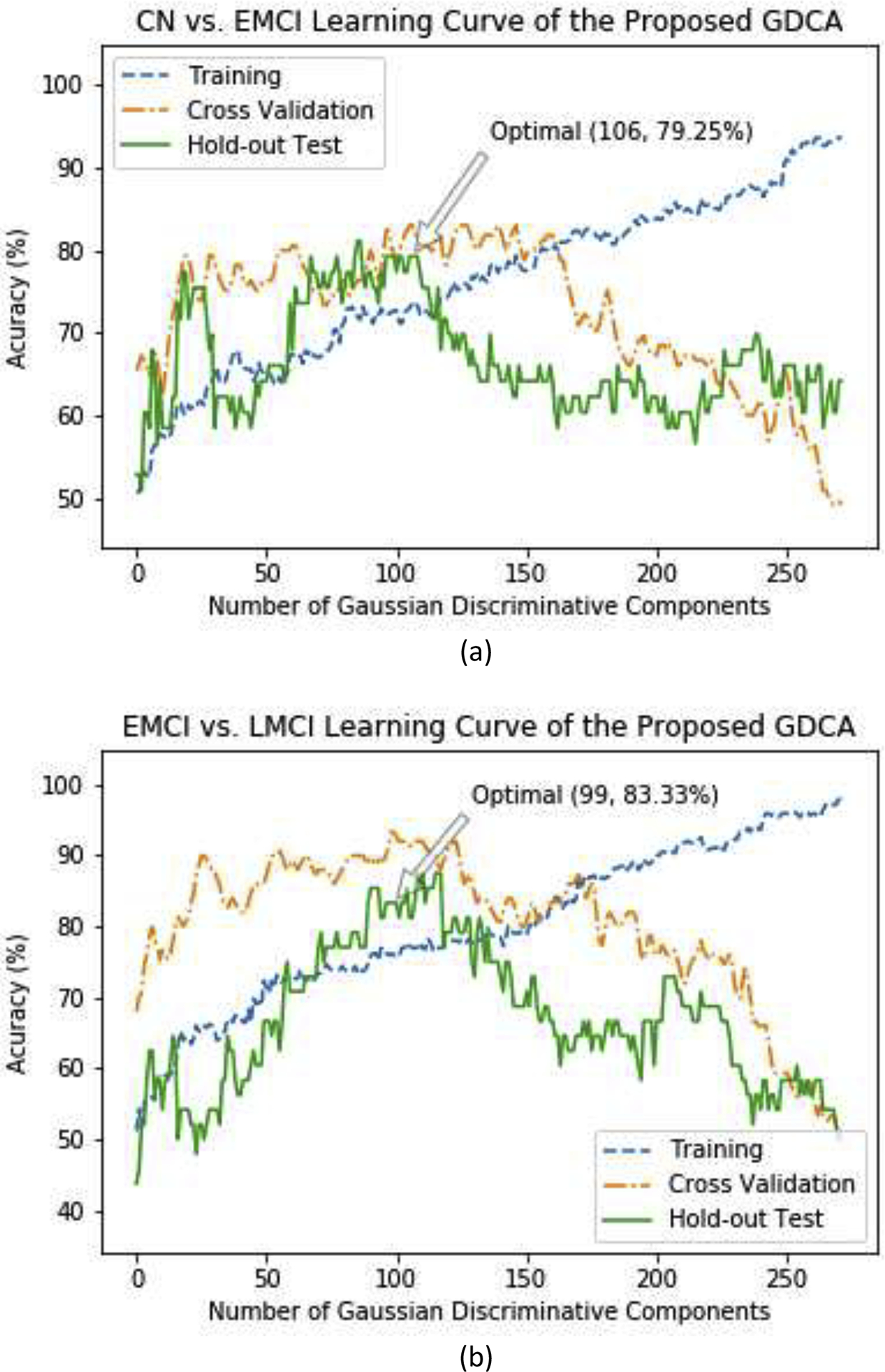
The learning curves of the training, validation and testing with different numbers of Gaussian discriminative components: (a) CN vs. EMCI classification; (b) EMCI vs. LMCI classification.
Table 3.
Benchmark CN vs. EMCI and EMCI vs. LMCI classification results based on the GDCA
| Classification | CN vs. EMCI | EMCI vs. LMCI | ||||||
|---|---|---|---|---|---|---|---|---|
| Performance | F1 Score | Accuracy | Precision | Recall | F1 Score | Accuracy | Precision | Recall |
| Cross validation | 86.15% | 83.64% | 80.00% | 93.33% | 92.31% | 94.00% | 94.74% | 90.00% |
| Hold-out test | 80.70% | 79.25% | 82.14% | 79.31% | 77.78% | 83.33% | 82.35% | 73.68% |
4.2. Binary Classification Performance Comparison
By applying the relevant classifiers (i.e., SVM, MLP, and GB) to the original data and to the dimensionality-reduced data, the corresponding results are given in Table 4. Unlike the proposed GDCA, these algorithms may give us various results due to the random initialization. The classification experiments were run multiple times on the best training/validation data split, and for each classifier, the best performing model was selected, then the corresponding test results were reported in Table 4. It can be observed that after introducing the proposed dimensionality reduction model, all the selected classifiers achieved better performance on the transformed feature space than obtained on the original features, which adds credence to the validity of the proposed GDCA model. Moreover, although state-of-the-art MLP and GB algorithms established better performance than the GDA algorithm on the original features as a result of the underlying feature selection process, for both CN vs. EMCI and EMCI vs. LMCI, they did not surpass the benchmark performance yielded by the proposed GDCA algorithm. However, because of the random initialization, classification algorithms like SVM, MPL, GB may not always achieve the global optimal solution, only the GDA classifier is applied here for the multiclass classification experiment.
Table 4.
Binary classification performance comparison of original features and GDCA-transformed features
| Task | Feature | Original Features | Transformed Features | ||||||
|---|---|---|---|---|---|---|---|---|---|
| Classifier | F1 Score | Accuracy | Precision | Recall | F1 Score | Accuracy | Precision | Recall | |
| CN vs. EMCI | SVM | 72.73% | 66.04% | 64.86% | 82.76% | 78.69% | 75.47% | 75.00% | 82.76% |
| MLP | 75.41% | 71.70% | 71.88% | 79.31% | 78.57% | 77.36% | 81.48% | 75.86% | |
| GB | 75.41% | 71.70% | 71.88% | 79.31% | 77.19% | 75.47% | 78.57% | 75.86% | |
| GDA | 66.67% | 64.15% | 67.86% | 65.52% | 80.70% | 79.25% | 82.14% | 79.31% | |
| EMCI vs. LMCI | SVM | 54.05% | 64.58% | 55.56% | 52.63% | 65.00% | 70.83% | 61.90% | 68.42% |
| MLP | 59.46% | 68.75% | 61.11% | 57.89% | 72.73% | 75.00% | 64.00% | 84.21% | |
| GB | 48.48% | 64.58% | 57.14% | 42.11% | 60.00% | 75.00% | 81.82% | 47.37% | |
| GDA | 52.00% | 50.00% | 41.94% | 68.42% | 77.78% | 83.33% | 82.35% | 73.68% | |
As another widely used metric in choosing binary classification models, the receiver operating characteristic (ROC) curve and the area under the curve (AUC) were used to measure the classification performance. The AUC score can reveal the discriminability of a classification model and to indicate if the false positive and true positive rates achieved by a model are significantly above random chance. The ROC curves and the corresponding AUC scores of hold-out tests on original and transformed feature spaces are demonstrated in Fig. 3, and it can be observed that, after carrying out the proposed GDCA model, the AUC scores improved significantly by 0.15 for CN vs. EMCI classification and by 0.31 for EMCI vs. LMCI classification.
Fig. 3.
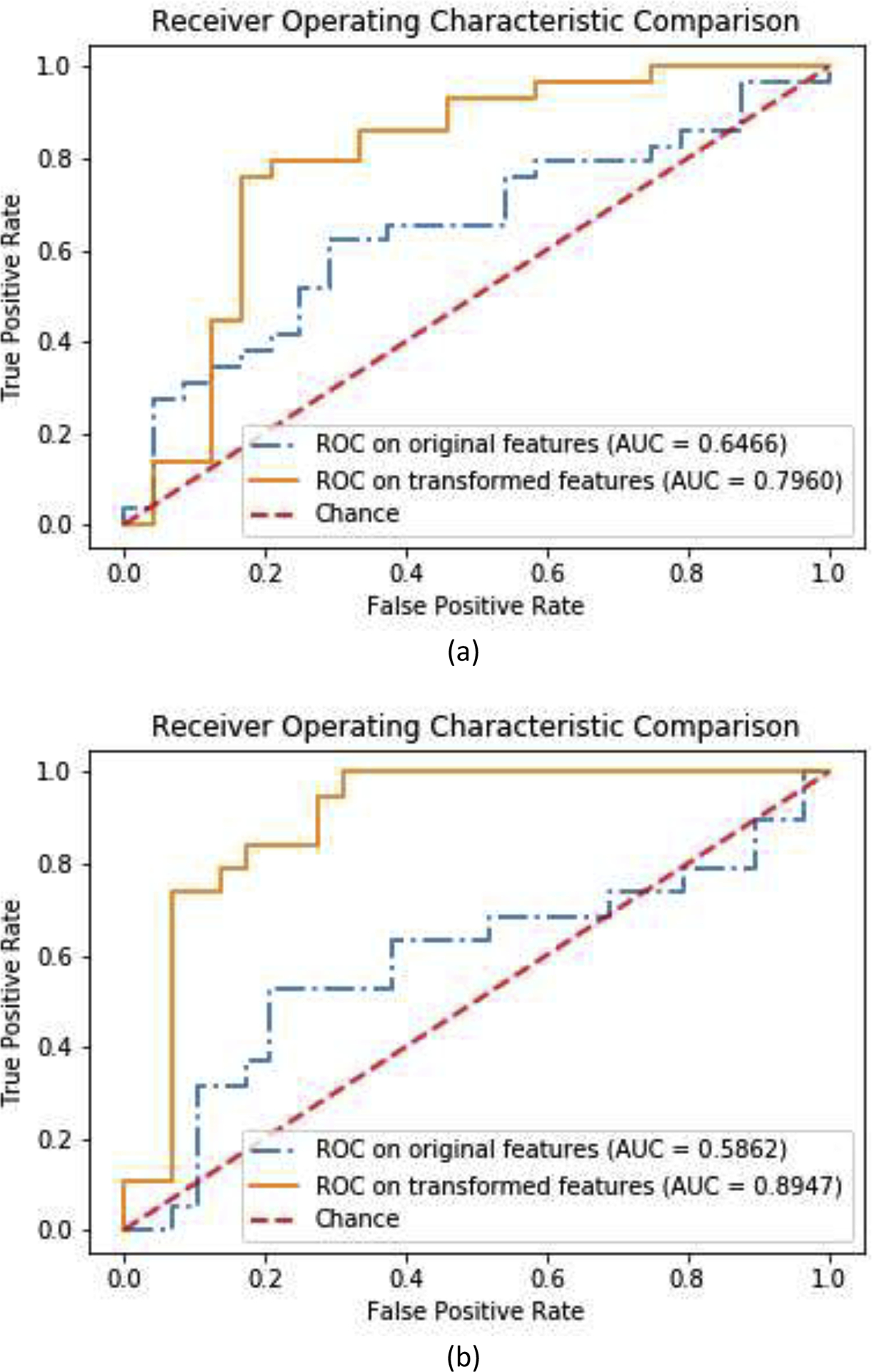
ROC curves and AUC scores on original features and GDCA transformed features: (a) CN vs. EMCI classification; (b) EMCI vs. LMCI classification.
In Table 5, the results obtained by the proposed GDCA model are compared with those obtained using most recent state-of-the-art methods based on ADNI data [30–36]. It should be noted that, as shown in Table 5, although most of the studies used relatively small dataset, the proposed model still achieved overall best performance for both CN vs. EMCI classification and EMCI vs. LMCI classification; and for the only study having the relatively large number of subjects [34], the proposed study obtained significantly better performance.
Table 5.
CN vs. EMCI and EMCI vs. LMCI classification performance comparison
| Classification | Subjects (CN/EMCI/LMCI) |
CN vs. EMCI | EMCI vs. LMCI | ||||||
|---|---|---|---|---|---|---|---|---|---|
| Performance | Accuracy | Sensitivity | Specificity | AUC | Accuracy | Sensitivity | Specificity | AUC | |
| Pei et al. [30], 2018 | -/18/18 | - | - | - | - | 70.00% | - | - | 0.7088 |
| Hett et al. [31], 2019 | 62/65/34 | - | - | - | - | 70.80% | - | - | 0.6240 |
| Jie et al. [32], 2018 | 50/56/43 | - | - | - | - | 74.80% | - | - | 0.7200 |
| Jie et al. [33], 2018 | 50/56/43 | 78.30% | 74.00% | 82.10% | 0.7710 | 78.80% | 82.10% | 74.40% | 0.7830 |
| Wee et al. [34], 2019 | 300/314/208 | 53.00% | 60.40% | 55.00% | - | 63.10% | 61.30% | 77.60% | - |
| Yang et al. [35] , 2019 | 29/29/18 | 77.59% | 59.09% | - | 0.6849 | 76.60% | 66.20% | - | 0.7682 |
| Kam et al. [36], 2019 | 48/49/- | 76.07% | 76.27% | 75.87% | - | - | - | - | - |
| Proposed | 251/297/196 | 79.25% | 79.31% | 79.17% | 0.7960 | 83.33% | 82.35% | 89.66% | 0.8947 |
4.3. EMCI vs. LMCI vs. AD Multiclass classification
The same pipeline was followed for the multiclass classification experiments, and since the F1 score, precision, and recall would no longer be available, the confusion matrix was used instead to evaluate the performance with each row corresponding to the true class. The diagonal elements of the confusion matrix represent the number of points for which the predicted label is equal to the true label, while off-diagonal elements are those that are misclassified by the classifier.
Fig. 4 demonstrates the learning curve of the multiclass classification experiment using the proposed GDCA, where the best cross validation performance was achieved by using the first 90 Gaussian discriminative component. It can be observed that the learning curve associated with the hold-out test is closer to the learning curve of cross validation in comparison to the learning curve results shown in Fig. 2, since there were three classes instead of two classes, which enabled the model to learn more generic discriminative components across all three classes.
Fig. 4.
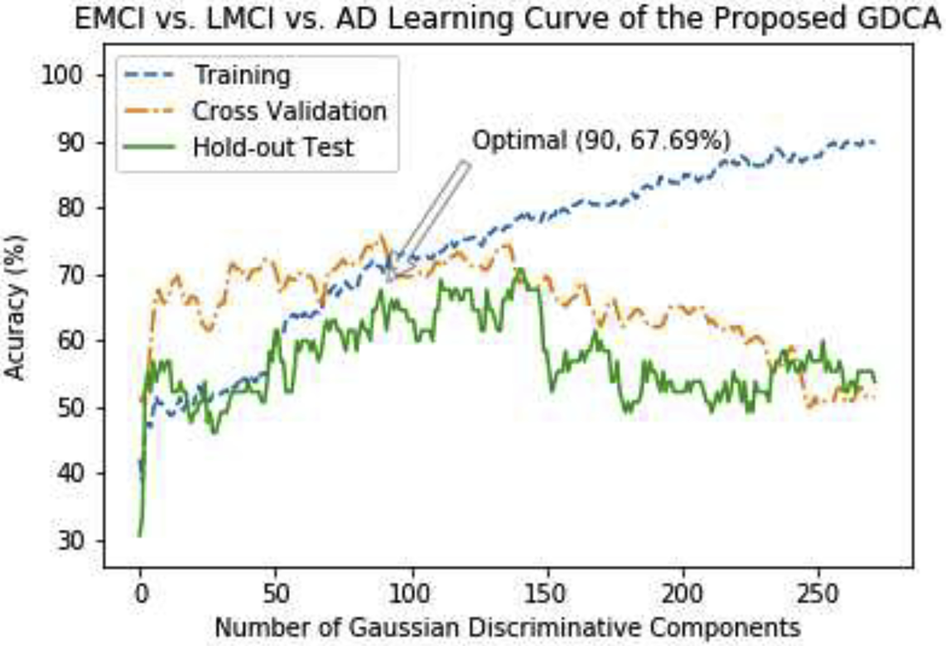
The learning curves of the training, validation and testing with different numbers of Gaussian discriminative components for EMCI vs. LMCI vs. AD classification.
Fig. 5 shows the confusion matrices of the hold-out test on the original features and GDCA transformed features. The overall classification accuracy using the transformed features was 67.69%, compared to 53.85% if all original features were utilized. As shown in Fig. 5, after applying the proposed GDCA model, the classifier could more precisely distinguish LMCI and AD from EMCI group, so that the overall classification performance was improved significantly. Additionally, Table 6 converted the multiclass classification results to binary classification results of MCI vs. AD, showing that the proposed method could effectively discriminate AD from MCI with a 31.25% increase on recall.
Fig. 5.
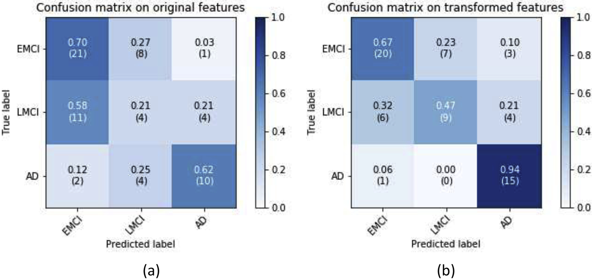
EMCI vs. LMCI vs. AD classification confusion matrices: (a) All features were used; (b) GDCA-transformed features were used.
Table 6.
MCI vs. AD classification performance by converting the EMCI vs. LMCI vs. AD classification results
| Features | F1 Score | Accuracy | Precision | Recall |
|---|---|---|---|---|
| Original | 64.52% | 83.08% | 66.67% | 62.50% |
| Transformed | 78.95% | 87.69% | 68.18% | 93.75% |
4.4. Dimensionality Reduction Performance Comparison
Since the proposed GDCA method is capable of defining the most discriminative directions of all eigenvectors, noted improvements were obtained in the classification results. To demonstrate how this process differs from other widely used dimensionality reduction methods, the same procedure was implemented for the EMCI vs. LMCI vs. AD multiclass classification task by applying the PCA, LASSO, univariate feature selection and proposed GDCA methods. The PCA method, as aforementioned, utilizes PCA computed variances to determine the significances of the principal components. Since linear models regularized with the L1 norm (i.e., LASSO) have sparse solutions, and the estimated coefficients could be employed in measuring the importance of each feature, therefore, which can also be used to select the most important features. For univariate selection method, the eigenvectors of the covariance matrix are not computed, and instead it selects the best features based on univariate statistical tests. In this study, the analysis of variance (ANOVA) was performed as the univariate statistical test to determine the significances of the different features.
Moreover, rather than adding one feature at a time, the different percentiles were used to illustrate the classification performance of these dimensionality reduction methods varying the percentile of features selected. The same GDA classifier was applied to all these four dimensionality reduction methods so as to eliminate any bias. Fig. 6 shows the 9-fold cross validation results of these methods.
Fig. 6.
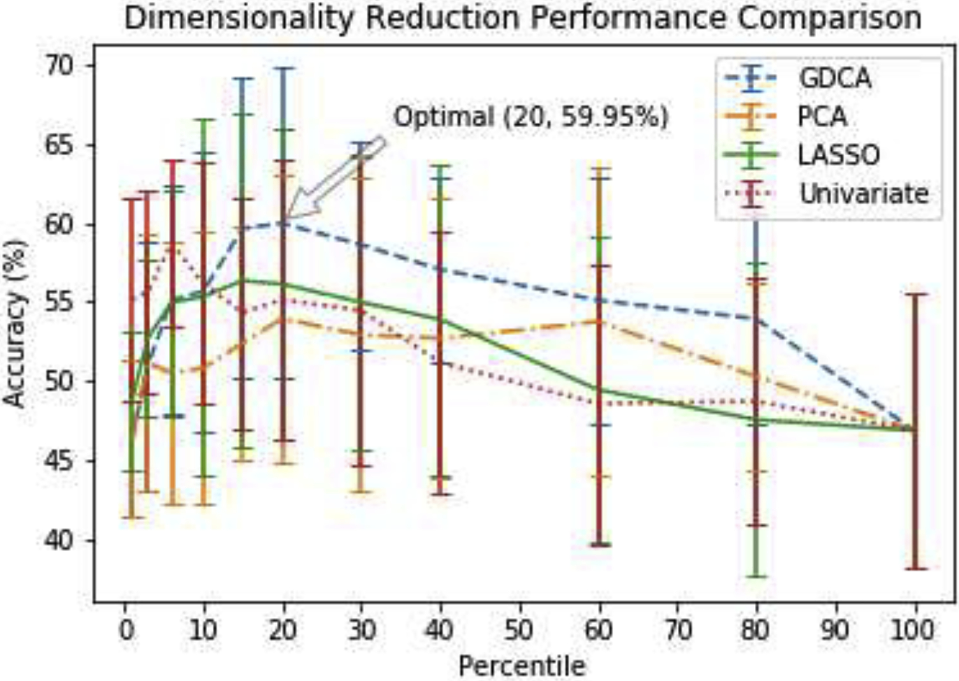
EMCI vs. LMCI vs. AD cross validation performance of different dimensionality reduction methods varying the percentile of features selected.
As can be observed from the results shown in Fig. 6, the ANOVA-based univariate selection method reached quickly an optimal average cross validation accuracy with 5% of the features used and seems to outperform all other methods when 10% or less of the features are used. The nature of the Univariate performance graph with its rapid decline in performance with more features included misses out on that optimal solution that is reached out by the proposed GDCA methods when 20% of the features are used. At 15% of the features used, both LASSO and GDCA performed well and they were better in performance than the PCA and the Univariate methods. However, with more features added, the decline in performance is more gradual in the proposed GDCA method than it is for LASSO.
Overall, the proposed GDCA method obtained an optimal hold-out test accuracy of 65.62% with 20 percent of all features, which is better than the hold-out test performance achieved by the LASSO (56.25%), the Univariate (57.81%) and the PCA (62.50%) methods. It also indicated that making use of the eigenspace rather than the original feature space could help the model attain more generally selected features to avoid overfitting on the training data, which resulted in better hold-out test performance yielded by the GDCA and the PCA methods.
4.5. Computer aided diagnosis based on GDCA
The previous sections have indicated that the proposed GDCA model was able to identify the most discriminative components associated with different stages of AD as a multiclass classification problem. But, in order to apply the proposed model to a practical CAD system, the trained model should be able to include the CN group, allowing a given subject in the classification process to belong to any of the 4 groups: CN, EMCI, LMCI and AD. Therefore, in this section, a multimodal multiclass classification neuroimaging CAD application involving all four groups (CN, EMCI, LMCI and AD) is presented utilizing the proposed GDCA model.
The learning curve of the GDCA-based CAD application is shown in Fig. 7, where the best cross validation performance was obtained by using the first 133 Gaussian discriminative components. Now, since more interclass information was involved during the training, more generic discriminative components across all four classes were captured, which resulted in a small gap between the learning curves of the cross validation and the hold-out test. Fig. 8 demonstrates the confusion matrices of the hold-out test on the original features and GDCA transformed features. As the most complicated task in AD classification, the accuracy of 53.93% was attained, which reached only 41.57% when all original features were used. Making use of GDA, Fig. 9 illustrates the 3-dimensional visualization by projecting the high dimensional data onto the affine subspace generated by the estimated class means of all classes. In Fig. 8 and Fig. 9, it can be observed that, after applying the proposed GDCA model, the classifier could detect the subtle difference between MCI group (i.e., EMCI and LMCI) and CN group as well as MCI group and AD group more effectively, in particular, more CN and AD subjects were correctly detected.
Fig. 7.
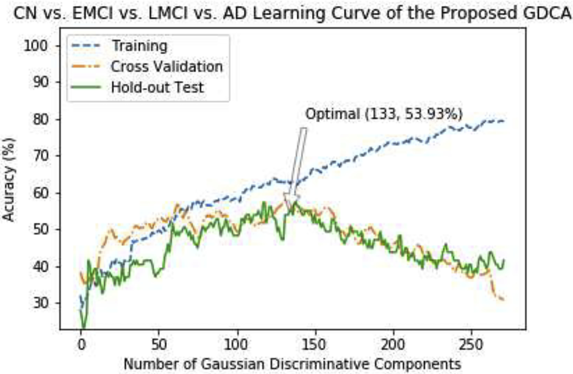
The learning curves of the training, validation and testing with different numbers of Gaussian discriminative components for the proposed GDCA-based CAD application.
Fig. 8.
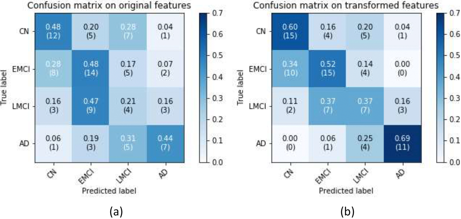
CN vs. EMCI vs. LMCI vs. AD classification confusion matrices: (a) All features were used; (b) GDCA-transformed features were used.
Fig. 9.
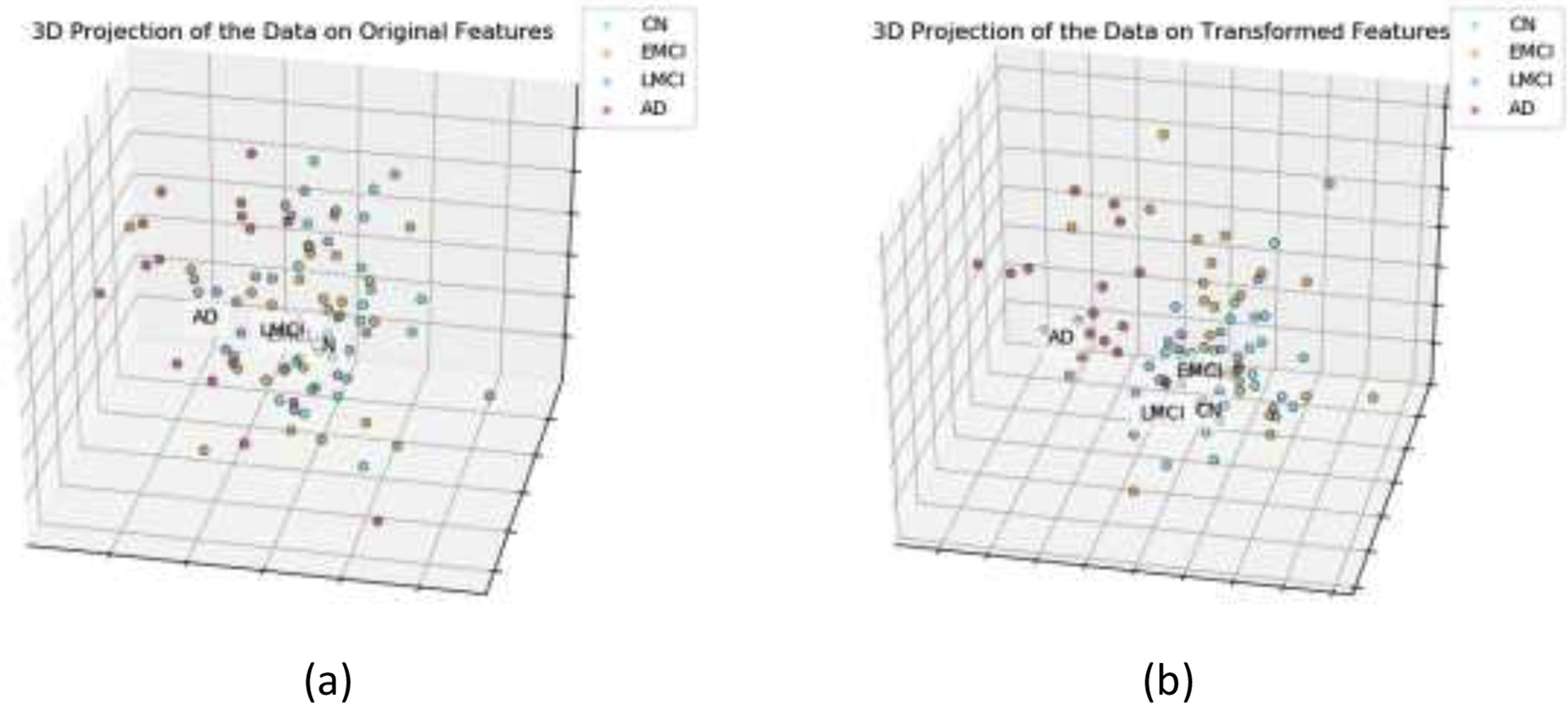
CN vs. EMCI vs. LMCI vs. AD 3-dimensional visualization by projecting the data onto the affine subspace: (a) All features were used; (b) GDCA-transformed features were used.
Furthermore, in order to illustrate the performance improvement of the GDCA-based CAD application, some extension of ROC to multiclass classification were carried out, including, one-against-rest ROC curve for each class, micro-averaging and macro-averaging ROC curves. Micro-averaging considers each element of the label indicator matrix as a binary prediction, while macro-averaging gives equal weight to the classification of each label. The ROC curves and the corresponding AUC scores are demonstrated in Fig. 10, and it can be observed that, after carrying out the proposed GDCA model, the micro-averaging and macro-averaging AUC scores were increased significantly by 9.71% and 8.73%, respectively. For AD vs. rest and CN vs. rest, the performances were also improved significantly, and AUC scores of 0.7919 and 0.9092, respectively were achieved.
Fig. 10.
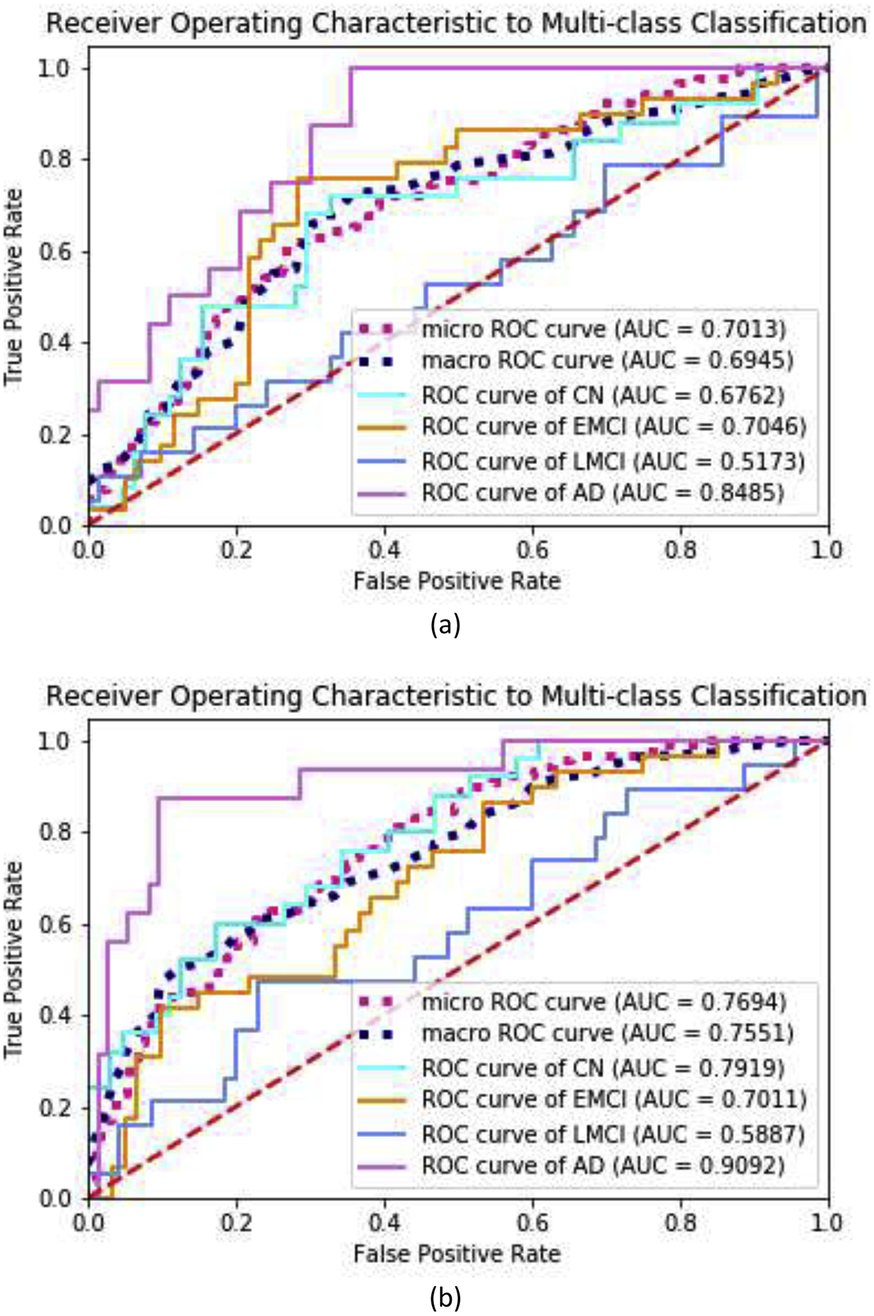
ROC curves to multiclass classification and AUC scores for the proposed GDCA-based CAD application: (a) All features were used; (b) GDCA-transformed features were used.
As shown in Fig. 9, after applying the GDCA model, the classification improvement was attributed to more of the CN and AD subjects correctly distinguished from EMCI and LMCI groups. Therefore, in order to demonstrate the performance improvement on CN vs. MCI vs. AD classification, the CAD results of EMCI and LMCI were combined together as MCI. By combining those results, the confusion matrices on the original features and GDCA transformed features are shown in Fig. 11. After combining, the overall classification accuracy on original and transformed features was 57.30% and 66.29%, respectively. And more notably, if the MCI and AD results were further combined as diseased group, it indicates that the proposed GDCA-based CAD application can effectively discriminate diseased subjects from the CN group with an accuracy of 75.28%, an F1 score of 82.51%, a precision of 83.87%, and a recall of 81.25%. These results show that the proposed GDCA model has a high potential for use as a clinical CAD system using multimodal neuroimaging data.
Fig. 11.
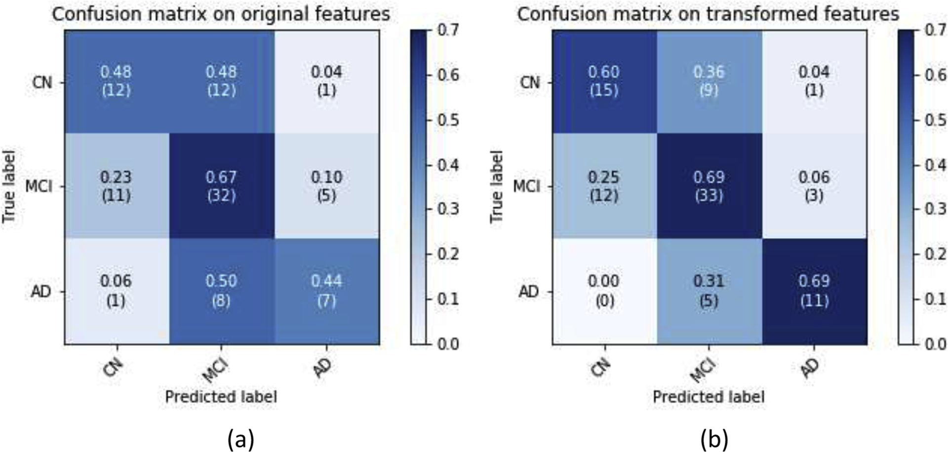
CN vs. MCI vs. AD classification confusion matrices by combining EMCI and LMCI: (a) All features were used; (b) GDCA-transformed features were used.
5. CONCLUSIONS
In this study, a novel GDCA dimensionality reduction algorithm was proposed to characterize the optimal Gaussian discriminative components of the original high dimensional feature space, maximizing as a consequence the discriminability of selected eigenvectors. The CN vs. EMCI classification results indicated that the proposed supervised method was able to delineate the subtlest changes associated with the EMCI group. After transforming the original features to the optimal Gaussian discriminative components, a high accuracy of 79.25%, an F1 score of 80.70% and an AUC score of 0.7960 were obtained, which showed high potential of the proposed method for clinical diagnosis of the early stage of AD. For EMCI vs. LMCI classification, the proposed model achieved a high accuracy of 83.33%, an F1 score of 77.78%, and an AUC score of 0.8947. These results of CN vs. EMCI classification and EMCI vs. LMCI classification are considered as the best classification performance obtained so far.
A multiclass classification was also carried out for the detection of the different stages in AD (i.e., EMCI, LMCI, and AD). An overall accuracy of 67.69% was achieved, and moreover, the proposed method was able to distinguish AD from MCI with an accuracy of 87.69% and a recall of 93.75%, respectively. The comparison with other widely used dimensionality reduction methods indicated that the proposed method could significantly reduce the dimensionality of the data and still accomplish an effective classification performance. A CAD application based on the proposed GDCA model was also presented, which attained an overall accuracy of 66.29% for CN vs. MCI vs. AD classification, and more notably, for distinguishing diseased subjects (i.e., MCI and AD) from CN group, with an accuracy of 75.28%. The future work will ultimately focus on taking advantage of the proposed GDCA algorithm to build a CAD system that could help in delineating the EMCI group in a multiclass classification process that could be helpful in the planning of early treatment and therapeutic interventions.
Highlights.
Introducing a novel supervised dimensionality reduction algorithm to characterize the optimal Gaussian discriminative components of the original high dimensional feature space.
Achieving the best classification performance of CN vs. EMCI and EMCI vs. LMCI classifications compared with most recent state-of-the-art methods.
Reducing the dimensionality of the data and still accomplishing more effective classification performance than other widely used dimensionality reduction methods.
Attaining an overall accuracy of 67.69% for CN vs. MCI vs. AD classification, and more notably, distinguishing diseased subjects (i.e., MCI and AD) from CN group with an accuracy of 75.28%.
ACKNOWLEDGEMENTS
Data collection and sharing for this project was funded by the Alzheimer’s Disease Neuroimaging Initiative (ADNI) (National Institutes of Health Grant U01 AG024904) and DOD ADNI (Department of Defense award number W81XWH-12-2-0012). ADNI is funded by the National Institute on Aging, the National Institute of Biomedical Imaging and Bioengineering, and through generous contributions from the following: AbbVie, Alzheimer’s Association; Alzheimer’s Drug Discovery Foundation; Araclon Biotech; BioClinica, Inc.; Biogen; Bristol-Myers Squibb Company; CereSpir, Inc.; Cogstate; Eisai Inc.; Elan Pharmaceuticals, Inc.; Eli Lilly and Company; EuroImmun; F. Hoffmann-La Roche Ltd and its affiliated company Genentech, Inc.; Fujirebio; GE Healthcare; IXICO Ltd.; Janssen Alzheimer Immunotherapy Research & Development, LLC.; Johnson & Johnson Pharmaceutical Research & Development LLC.; Lumosity; Lundbeck; Merck & Co., Inc.; Meso Scale Diagnostics, LLC.; NeuroRx Research; Neurotrack Technologies; Novartis Pharmaceuticals Corporation; Pfizer Inc.; Piramal Imaging; Servier; Takeda Pharmaceutical Company; and Transition Therapeutics. The Canadian Institutes of Health Research is providing funds to support ADNI clinical sites in Canada. Private sector contributions are facilitated by the Foundation for the National Institutes of Health (www.fnih.org). The grantee organization is the Northern California Institute for Research and Education, and the study is coordinated by the Alzheimer’s Therapeutic Research Institute at the University of Southern California. ADNI data are disseminated by the Laboratory for Neuro Imaging at the University of Southern California.
We are grateful for the continued support from the National Science Foundation (NSF) under NSF grants CNS-1920182, CNS-1532061, CNS-1338922, and CNS-1551221. We also greatly appreciate the support of NIH-NIA grants (1R01AG055638-01A1, 1R01AG061106-01), State of Florida grant (8AZ23), the 1Florida Alzheimer’s Disease Research Center (ADRC) (NIA 1P50AG047266-01A1) and the Ware Foundation.
Footnotes
Publisher's Disclaimer: This is a PDF file of an unedited manuscript that has been accepted for publication. As a service to our customers we are providing this early version of the manuscript. The manuscript will undergo copyediting, typesetting, and review of the resulting proof before it is published in its final form. Please note that during the production process errors may be discovered which could affect the content, and all legal disclaimers that apply to the journal pertain.
References
- [1].Khedher L, Ramirez J, Gorriz J, Brahim A, Segovia F, Initia ADN (2015) Early diagnosis of Alzheimer’s disease based on partial least squares, principal component analysis and support vector machine using segmented MRI images. Neurocomputing 151, 139–150. [Google Scholar]
- [2].Ofori E, DeKosky ST, Febo M, Colon-Perez L, Chakrabarty P, Duara R, Adjouadi M, Golde TE, Vaillancourt DE, Initiative AsDN (2019) Free-water imaging of the hippocampus is a sensitive marker of Alzheimer’s disease. Neuroimage Clin 24, 101985. [DOI] [PMC free article] [PubMed] [Google Scholar]
- [3].Vaithinathan K, Parthiban L, Initiative AsDN (2019) A Novel Texture Extraction Technique with T1 Weighted MRI for the Classification of Alzheimer’s Disease. J Neurosci Methods 318, 84–99. [DOI] [PubMed] [Google Scholar]
- [4].Tabarestani S, Aghili M, Eslami M, Cabrerizo M, Barreto A, Rishe N, Curiel RE, Loewenstein D, Duara R, Adjouadi M (2019) A distributed multitask multimodal approach for the prediction of Alzheimer’s disease in a longitudinal study. Neuroimage, 116317. [DOI] [PMC free article] [PubMed] [Google Scholar]
- [5].Forouzannezhad P, Abbaspour A, Li C, Fang C, Williams U, Cabrerizo M, Barreto A, Andrian J, Rishe N, Curiel RE, Loewenstein D, Duara R, Adjouadi M (2019) A Gaussian-based model for early detection of mild cognitive impairment using multimodal neuroimaging. J Neurosci Methods 333, 108544. [DOI] [PMC free article] [PubMed] [Google Scholar]
- [6].Fang C, Li C, Cabrerizo M, Barreto A, Andrian J, Rishe N, Loewenstein D, Duara R, Adjouadi M (2018) Gaussian Discriminant Analysis for Optimal Delineation of Mild Cognitive Impairment in Alzheimer’s Disease. Int J Neural Syst 28, 1850017. [DOI] [PubMed] [Google Scholar]
- [7].Moradi E, Pepe A, Gaser C, Huttunen H, Tohka J, Initiative AsDN (2015) Machine learning framework for early MRI-based Alzheimer’s conversion prediction in MCI subjects. Neuroimage 104, 398–412. [DOI] [PMC free article] [PubMed] [Google Scholar]
- [8].Zhang D, Shen D, Initiative AsDN (2012) Multi-modal multi-task learning for joint prediction of multiple regression and classification variables in Alzheimer’s disease. Neuroimage 59, 895–907. [DOI] [PMC free article] [PubMed] [Google Scholar]
- [9].Chu C, Hsu AL, Chou KH, Bandettini P, Lin C, Initiative AsDN (2012) Does feature selection improve classification accuracy? Impact of sample size and feature selection on classification using anatomical magnetic resonance images. Neuroimage 60, 59–70. [DOI] [PubMed] [Google Scholar]
- [10].Liu F, Wee CY, Chen H, Shen D (2014) Inter-modality relationship constrained multi-modality multi-task feature selection for Alzheimer’s Disease and mild cognitive impairment identification. Neuroimage 84, 466–475. [DOI] [PMC free article] [PubMed] [Google Scholar]
- [11].Zhu X, Suk HI, Wang L, Lee SW, Shen D, Initiative AsDN (2017) A novel relational regularization feature selection method for joint regression and classification in AD diagnosis. Med Image Anal 38, 205–214. [DOI] [PMC free article] [PubMed] [Google Scholar]
- [12].Ota K, Oishi N, Ito K, Fukuyama H, Group S-JS, Initiative AsDN (2015) Effects of imaging modalities, brain atlases and feature selection on prediction of Alzheimer’s disease. J Neurosci Methods 256, 168–183. [DOI] [PubMed] [Google Scholar]
- [13].Li C, Duara R, Loewenstein DA, Izquierdo W, Cabrerizo M, Barker W, Adjouadi M, Initiative aftAsDN (2019) Greater Regional Cortical Thickness is Associated with Selective Vulnerability to Atrophy in Alzheimer’s Disease, Independent of Amyloid Load and APOE Genotype. J Alzheimers Dis 69, 145–156. [DOI] [PubMed] [Google Scholar]
- [14].Loewenstein DA, Curiel RE, DeKosky S, Rosselli M, Bauer R, Grieg-Custo M, Penate A, Li C, Lizagarra G, Golde T, Adjouadi M, Duara R (2017) Recovery from Proactive Semantic Interference and MRI Volume: A Replication and Extension Study. J Alzheimers Dis 59, 131–139. [DOI] [PMC free article] [PubMed] [Google Scholar]
- [15].Plant C, Teipel SJ, Oswald A, Böhm C, Meindl T, Mourao-Miranda J, Bokde AW, Hampel H, Ewers M (2010) Automated detection of brain atrophy patterns based on MRI for the prediction of Alzheimer’s disease. Neuroimage 50, 162–174. [DOI] [PMC free article] [PubMed] [Google Scholar]
- [16].Zhang F, Tian S, Chen S, Ma Y, Li X, Guo X (2019) Voxel-Based Morphometry: Improving the Diagnosis of Alzheimer’s Disease Based on an Extreme Learning Machine Method from the ADNI cohort. Neuroscience 414, 273–279. [DOI] [PubMed] [Google Scholar]
- [17].Sun X, Liang S, Fu L, Zhang X, Feng T, Li P, Zhang T, Wang L, Yin X, Zhang W, Hu Y, Liu H, Zhao S, Nie B, Xu B, Shan B (2019) A human brain tau PET template in MNI space for the voxel-wise analysis of Alzheimer’s disease. J Neurosci Methods 328, 108438. [DOI] [PubMed] [Google Scholar]
- [18].Ossenkoppele R, Jansen WJ, Rabinovici GD, Knol DL, van der Flier WM, van Berckel BN, Scheltens P, Visser PJ, Verfaillie SC, Zwan MD, Adriaanse SM, Lammertsma AA, Barkhof F, Jagust WJ, Miller BL, Rosen HJ, Landau SM, Villemagne VL, Rowe CC, Lee DY, Na DL, Seo SW, Sarazin M, Roe CM, Sabri O, Barthel H, Koglin N, Hodges J, Leyton CE, Vandenberghe R, van Laere K, Drzezga A, Forster S, Grimmer T, Sánchez-Juan P, Carril JM, Mok V, Camus V, Klunk WE, Cohen AD, Meyer PT, Hellwig S, Newberg A, Frederiksen KS, Fleisher AS, Mintun MA, Wolk DA, Nordberg A, Rinne JO, Chételat G, Lleo A, Blesa R, Fortea J, Madsen K, Rodrigue KM, Brooks DJ, Group APS (2015) Prevalence of amyloid PET positivity in dementia syndromes: a meta-analysis. JAMA 313, 1939–1949. [DOI] [PMC free article] [PubMed] [Google Scholar]
- [19].Farzan A, Mashohor S, Ramli A, Mahmud R (2015) Boosting diagnosis accuracy of Alzheimer’s disease using high dimensional recognition of longitudinal brain atrophy patterns. Behavioural Brain Research 290, 124–130. [DOI] [PubMed] [Google Scholar]
- [20].Lopez M, Ramirez J, Gorriz J, Alvarez I, Salas-Gonzalez D, Segovia F, Chaves R, Padilla P, Gomez-Rio M, Neuroimaging AsD (2011) Principal component analysis-based techniques and supervised classification schemes for the early detection of Alzheimer’s disease. Neurocomputing 74, 1260–1271. [Google Scholar]
- [21].Curiel Cid RE, Loewenstein DA, Rosselli M, Matias-Guiu JA, Piña D, Adjouadi M, Cabrerizo M, Bauer RM, Chan A, DeKosky ST, Golde T, Greig-Custo MT, Lizarraga G, Peñate A, Duara R (2019) A cognitive stress test for prodromal Alzheimer’s disease: Multiethnic generalizability. Alzheimers Dement (Amst) 11, 550–559. [DOI] [PMC free article] [PubMed] [Google Scholar]
- [22].Loewenstein DA, Curiel RE, DeKosky S, Bauer RM, Rosselli M, Guinjoan SM, Adjouadi M, Peñate A, Barker WW, Goenaga S, Golde T, Greig-Custo MT, Hanson KS, Li C, Lizarraga G, Marsiske M, Duara R (2018) Utilizing semantic intrusions to identify amyloid positivity in mild cognitive impairment. Neurology 91, e976–e984. [DOI] [PMC free article] [PubMed] [Google Scholar]
- [23].Curiel RE, Loewenstein DA, Rosselli M, Penate A, Greig-Custo MT, Bauer RM, Guinjoan SM, Hanson KS, Li C, Lizarraga G, Barker WW, Torres V, DeKosky S, Adjouadi M, Duara R (2018) Semantic Intrusions and Failure to Recover From Semantic Interference in Mild Cognitive Impairment: Relationship to Amyloid and Cortical Thickness. Curr Alzheimer Res 15, 848–855. [DOI] [PMC free article] [PubMed] [Google Scholar]
- [24].Duara R, Loewenstein DA, Lizarraga G, Adjouadi M, Barker WW, Greig-Custo MT, Rosselli M, Penate A, Shea YF, Behar R, Ollarves A, Robayo C, Hanson K, Marsiske M, Burke S, Ertekin-Taner N, Vaillancourt D, De Santi S, Golde T, St D (2019) Effect of age, ethnicity, sex, cognitive status and APOE genotype on amyloid load and the threshold for amyloid positivity. Neuroimage Clin 22, 101800. [DOI] [PMC free article] [PubMed] [Google Scholar]
- [25].Li C, Loewenstein DA, Duara R, Cabrerizo M, Barker W, Adjouadi M, Initiative AsDN (2017) The Relationship of Brain Amyloid Load and APOE Status to Regional Cortical Thinning and Cognition in the ADNI Cohort. J Alzheimers Dis 59, 1269–1282. [DOI] [PMC free article] [PubMed] [Google Scholar]
- [26].Westman E, Aguilar C, Muehlboeck JS, Simmons A (2013) Regional magnetic resonance imaging measures for multivariate analysis in Alzheimer’s disease and mild cognitive impairment. Brain Topogr 26, 9–23. [DOI] [PMC free article] [PubMed] [Google Scholar]
- [27].Jenkinson M, Beckmann C, Behrens T, Woolrich M, Smith S (2012) FSL. Neuroimage 62, 782–790. [DOI] [PubMed] [Google Scholar]
- [28].Li C, Fang C, Cabrerizo M, Barreto A, Andrian J, Duara R, Loewenstein D, Adjouadi M, Initi AsDN, Hu X, Shyu C, Bromberg Y, Gao J, Gong Y, Korkin D, I Y, Zheng J (2017) Pattern analysis of the interaction of regional amyloid load, cortical thickness and APOE genotype in the progression of Alzheimer’s disease. 2017 Ieee International Conference on Bioinformatics and Biomedicine (Bibm), 2171–2176. [Google Scholar]
- [29].Pedregosa F, Varoquaux G, Gramfort A, Michel V, Thirion B, Grisel O, Blondel M, Prettenhofer P, Weiss R, Dubourg V, Vanderplas J, Passos A, Cournapeau D, Brucher M, Perrot M, Duchesnay E (2011) Scikit-learn: Machine Learning in Python. Journal of Machine Learning Research 12, 2825–2830. [Google Scholar]
- [30].Pei S, Guan J, Zhou S (2018) Classifying early and late mild cognitive impairment stages of Alzheimer’s disease by fusing default mode networks extracted with multiple seeds. BMC Bioinformatics 19, 523. [DOI] [PMC free article] [PubMed] [Google Scholar]
- [31].Hett K, Ta VT, Catheline G, Tourdias T, Manjón JV, Coupé P, Initiative AsDN (2019) Multimodal Hippocampal Subfield Grading For Alzheimer’s Disease Classification. Sci Rep 9, 13845. [DOI] [PMC free article] [PubMed] [Google Scholar]
- [32].Jie B, Liu M, Zhang D, Shen D (2018) Sub-Network Kernels for Measuring Similarity of Brain Connectivity Networks in Disease Diagnosis. IEEE Trans Image Process 27, 2340–2353. [DOI] [PMC free article] [PubMed] [Google Scholar]
- [33].Jie B, Liu M, Shen D (2018) Integration of temporal and spatial properties of dynamic connectivity networks for automatic diagnosis of brain disease. Med Image Anal 47, 81–94. [DOI] [PMC free article] [PubMed] [Google Scholar]
- [34].Wee C, Liu C, Lee A, Poll J, Ji H, Qi A, Initiati ADN (2019) Cortical graph neural network for AD and MCI diagnosis and transfer learning across populations. Neuroimage-Clinical 23. [DOI] [PMC free article] [PubMed] [Google Scholar]
- [35].Yang P, Zhou F, Ni D, Xu Y, Chen S, Wang T, Lei B (2019) Fused Sparse Network Learning for Longitudinal Analysis of Mild Cognitive Impairment. IEEE Trans Cybern. [DOI] [PubMed] [Google Scholar]
- [36].Kam TE, Zhang H, Jiao Z, Shen D (2019) Deep Learning of Static and Dynamic Brain Functional Networks for Early MCI Detection. IEEE Trans Med Imaging. [DOI] [PMC free article] [PubMed] [Google Scholar]


