

Abstract
Mental health disorders have become a global problem, garnering considerable attention. However, the root causes of deteriorating mental health remain poorly understood, with existing literature predominantly concentrating on socioeconomic conditions and psychological factors. This study uses multi‐linear and geographically weighted regressions (GWR) to examine the associations between built and natural environmental attributes and the prevalence of depression in US counties. The findings reveal that job sprawl and land mixed use are highly correlated with a lower risk of depression. Additionally, the presence of green spaces, especially in urban area, is associated with improved mental health. Conversely, higher concentrations of air pollutants, such as PM2.5 and CO, along with increased precipitation, are linked to elevated depression rates. When considering spatial correlation through GWR, the impact of population density and social capital on mental health displays substantial spatial heterogeneity. Further analysis, focused on two high depression risk clustering regions (northwestern and southeastern counties), reveals nuanced determinants. In northwestern counties, depression rates are more influenced by factors like precipitation and socioeconomic conditions, including unemployment and income segregation. In southeastern counties, population demographic characteristics, particularly racial composition, are associated with high depression prevalence, followed by built environment factors. Interestingly, job growth and crime rates only emerge as significant factors in the context of high depression risks in southeastern counties. This study underscores the robust linkages and spatial variations between built and natural environments and mental health, emphasizing the need for effective depression treatment to incorporate these multifaceted factors.
Keywords: built environment, natural environment, socioeconomic conditions, mental health, spatial disparity
Key Points
Job sprawl, land mixed use, and green space associate with lower depression risk; the roles of air pollution and precipitation are opposite
Association of population density and social capital with depression prevalence exhibit significant spatial diversity
Precipitation and socioeconomic status mainly affect northwestern counties; population demographics plays key role in southeastern counties
1. Introduction
A significant number of US residents experience mental health problems, a burden that has intensified amidst the socioeconomic strains and public health crisis brought about by COVID‐19. The impact is substantial, with nearly 10 percent of US adults experiencing major depression each year and a recent global rise in depression rates (Moreno‐Agostino et al., 2021). Depression carries a range of socioeconomic and health repercussions, including the reduction of social capacity, a decline in labor productivity, and an increase in disability rates (Garrido‐Cumbrera et al., 2018). Notably, it stands as the most widespread psychiatric disorder associated with suicide mortality (Hawton et al., 2013). Given this high prevalence and the substantial costs, identifying place‐based risk factors of depression is imperative.
At individual‐level, risk of mental health problems is intricately linked to demographic characteristics, encompassing factors like genes, gender, and age, etc. (Silva et al., 2016). Due to biological, familial and sociocultural factors, women experience higher depression rates than men (Parker & Brotchie, 2010). Depressive symptoms in middle‐aged adults are significantly higher than in children and older adults (Cuijpers et al., 2020), because they usually have more anxiety and stress from financial status, work environment, and household relationship (Guan et al., 2022). A higher level of education may expose individuals to greater academic, social, and financial stress, which is linked to poor mental health (McCloud et al., 2023). Cvetkovski et al. (2019) reached the opposite conclusion. Single parents usually have lower income levels and are more likely to experience prejudice in society and mental health problems (Kim & Kim, 2020). Individual socio‐economic status can also significantly affect mental health. Individuals with low income disproportionately encounter economic and social stressors and have lower access to health and social resources (Marmot & Wilkinson, 2001). Unemployed people are linked to poor mental health because of financial and mental stress (McKee‐Ryan et al., 2005). Black/African Americans report greater psychological distress and more depressive symptoms (Barnes & Bates, 2017). Non‐Hispanic white Americans generally experience higher rates of major depressive disorder than African and Mexican Americans (Pamplin & Bates, 2021).
At area‐level, extensive research has shown that socioeconomic conditions impact mental well‐being (Lorant et al., 2003; Richardson et al., 2015). Places with higher social capital generally have lower rates of mental health disorders, due to emotional support and resources sharing (Thoits, 2011). However, close social ties can limit individual freedom and welfare and lead individuals to engage in health‐compromising behaviors such as alcohol consumption (Almedom, 2005). Limited health insurance coverage decreases access to mental health services and elevates mental health problems (Finkelstein et al., 2012). Residing in areas with more crimes reduces physical activity, decreases feelings of safety and increases risk of depression (Ross, 2017; Wei et al., 2021).
In recent years, the exploration of area‐level determinants has expanded to encompass physical and natural features within the built environment or urban form due to the acceleration and expansion of urbanization. Evidence indicates that urbanization contributes to psychological distress, and urban areas and larger cities tend to have higher rates of mental disorders (J. Chen et al., 2015). On the other hand, better infrastructure and public services in urban areas may increase residents' life satisfaction, thus improving their mental health (Stier et al., 2021). With the rise of urban sprawl as a global phenomenon, the process and effects of urban sprawl have drawn broad attention. Urban sprawl has been widely criticized for its association with various urban challenges, including imbalanced jobs‐housing distribution, traffic congestion, air pollution, diminished social cohesion, sedentary lifestyles, and adverse health outcomes (Wei & Ewing, 2018). Urban sprawl also contributes to residential segregation between different racial, ethnic, or socioeconomic groups, a spatial mismatch between low‐income households and suitable employment opportunities, and higher poverty rates among Black/African Americans. Consequently, urban sprawl is often considered a fundamental driver of urban problems in the US and is believed to have negative implications for mental health. The diversity of land use and job opportunities can enhance residents' access to resources, services, and employment opportunities, thereby meeting their daily needs and reducing psychological stress (Van Hooff & Van Hooft, 2014; Wu et al., 2016).
However, a study by Garrido‐Cumbrera et al. (2018) found that sprawling areas usually have fewer mental health problems, since households with more socioeconomic resources and lower risk of depression prefer less dense suburban areas with more natural resources (Brueckner et al., 1999; Curtis et al., 2024). Similarly, more dense neighborhoods tend to generate greater mental distress (Wang et al., 2021). Despite the importance of the built environment in shaping mental health outcomes, there is still a limited body of empirical research examining its impact.
Natural environmental conditions also influence mental health and are linked to the built environment. Air pollution, a byproduct of urban sprawl and increased vehicle miles traveled, exacerbates psychological distress (F. Chen et al., 2023; Piracha & Chaudhary, 2022), while green spaces and urban parks are stress‐relieving remedies (Richardson et al., 2013; Sturm & Cohen, 2014). Interestingly, the quality of green spaces appears to be more influential than the quantity in terms of their impact on mental health (Astell‐Burt et al., 2014). Moreover, the impact of green spaces on mental health has been found to vary between urban and rural areas (Ryan et al., 2024). Exposure to environmental toxins is another area‐level factor that heightens the risk of mental health disorders (McLeod, 2017).
Previous studies have investigated the mental health implications of various factors, including demographic characteristics, socioeconomic conditions, the built environment, and the natural environment (Dang et al., 2019; Li & Wei, 2023; Wang et al., 2021). However, a gap persists in terms of an inclusive research framework that integrates these influencing factors. Some argue that the contextual influence on mental health is primarily rooted in area socioeconomic conditions, overshadowing the significance of the built environment (Garrido‐Cumbrera et al., 2018). The role of the urban context in mental health remains inadequately elucidated, and scholars disagree about the definition of urban form or the built environment and their specific impacts on mental health (Clifton et al., 2008). Furthermore, the impacts of the natural environment, including air pollution and green spaces, have not been sufficiently explored (Mantler & Logan, 2015). Thus, we aim to advance the research on mental health by conducting a comprehensive study of the role of the built and natural environments in shaping mental health outcomes. Furthermore, our study contributes to existing knowledge by incorporating spatial perspectives to better grasp the spatial heterogeneity of mental health problems.
This paper provides a comprehensive understanding of the diverse area‐level risk factors for depression prevalence rates across US counties by analyzing the effects of built and natural environmental attributes. We ask the following research questions: (a) Where in the US is depression prevalence elevated? (b) How do built and natural environments contribute to variation in depression prevalence rates? (c) Do the predictors of depression prevalence vary across regions? To examine these questions, we compile a large data set that incorporates county‐level depression prevalence estimates for 2019 from the CDC Places, along with data from various publicly available sources capturing an extensive array of built and natural environmental attributes. Our analysis aims to shed light on the multifaceted causes of depression, providing valuable insights into the interplay between environmental factors and mental health outcomes.
2. Analytical Framework and Methodology
2.1. Analytical Framework
Building upon the literature review, this study integrates built and natural environments with demographic factors and socioeconomic conditions. The aim is to provide a more comprehensive understanding of the underlying causes of depression across US counties. The analytical framework is presented in Figure 1.
Figure 1.

The influencing factors of depression.
Studies tend to use one or two simple indicators such as population density or urban sprawl index to study the effects of built environment on health. Built environment covers multiple dimensions, and its comprehensive effects on mental health have rarely been thoroughly examined. Research on the effects of cities on human mobility and physical activities has predominantly focused on the built environment, mainly the three Ds (density, distance, and diversity). More recently, two more Ds (destination and design) have been incorporated into measures of urban form. These five Ds provide a comprehensive framework for understanding the influence of the built environment on human mobility, physical activity, and potentially mental health. We thus use a series of indices to represent built environment, including job sprawl index, population sprawl index, land mixed use index, job mixed layout index, job‐housing balance index, population density and urban area. Green space, pollutant PM2.5 and CO concentrations and precipitation are used to reflect the natural environment. Most studies find exposure to air pollution and increased precipitation are linked to more mental health problems, while green spaces can alleviate negative emotions (F. Chen et al., 2023; Kent et al., 2009; Leslie & Cerin, 2008; Sturm & Cohen, 2014). Our analytical framework also includes those typical natural environmental attributes.
Our research framework also incorporates control variables to reduce inaccurate model estimation due to omitted variables. Individual characteristics such as gender, aging, marital status, race and family structure affect mental health (Cuijpers et al., 2020; Pamplin & Bates, 2021; Parker & Brotchie, 2010). Socioeconomic conditions also play important roles in mental health. Usually, places with larger income segregation, lower job growth, higher unemployment rates, limited access to stores, less social capital, low health insurance coverage, and more crimes tend to have more mental health problems (McKee‐Ryan et al., 2005).
2.2. Data Sources
This study uses county level data for the continental US (i.e., excluding Alaska, Hawaii, and the US Territories). The US is among the countries with the most serious mental health related problems, and its cities are characterized by significant sprawling (Behnisch et al., 2022; Tikkanen et al., 2020). County diagnosed depression prevalence among adults came from the Centers for Disease Control and Prevention (CDC) Places, 2021 data release. CDC Places estimates of depression prevalence were derived from the Behavioral Risk Factor Surveillance System 2019 data using small area estimation techniques. County population estimates for subgroups were used to generate model‐based estimates of overall county depression prevalence among adults aged at least 18‐years‐old. The data and modeling approach are described in greater detail in Greenlund et al. (2022). In sensitivity tests, we used an age‐adjusted estimate for depression prevalence among adults to test the robustness of our results. Data representing built and natural environments, demographic factors, and socioeconomic conditions come from multiple publicly available sources. Table 1 presents detailed information on variable definitions and data sources. Additionally, we propose hypothesized associations for variables exhibiting relatively consistent findings based on the literature review.
Table 1.
Variable Selection and Data Sources
| Type | Abbreviation | Indicator meaning | Data sources |
|---|---|---|---|
| Depression | Dep | Depression rate. Model‐based estimate for crude prevalence of depression among adults aged 18–64 years (2019) | Disease Control and Prevention (CDC) |
| Dep2 | Age‐adjusted depression rate. Model‐based estimate for age‐adjusted crude prevalence of depression among adults aged 18–64 years (2019) | ||
| Built Environment | Sprawl_J | Job sprawl. Centering_coefficient of variation in census block group employment densities (2010). The more variation in densities around the mean, the more centering and/or subcentering exists within the county | Smart Location Database (SLD) Version 2.0 |
| Sprawl_P | Population sprawl. Centering_coefficient of variation in census block group population densities (2010). The more variation in densities around the mean, the more centering and/or subcentering exists within the county | ||
| Mixed_Land | Land mixed use. 5‐tier employment and household entropy. Values were weighted by the sum of block group's population and employment as a percentage of the county total (2010) | ||
| Mixed_Job | Job mixed layout. 5‐tier employment entropy, weighted by the sum of CBG population and employment as a percentage of the county total (2010) | ||
| Balance_JH | Jobs‐housing balance. Working population and actual jobs equilibrium Index, weighted by the sum of block group's population and employment as a percentage of the county total (2010). The closer to one the more balanced the resident workers and jobs in the Census Block Group | ||
| Density_P | Population density. Gross population density (people/acre) on unprotected land (2010) | ||
| Urban | Urban area. 1 is urban area, and 0 is non‐urban area | ||
| Natural Environment | Green_S | Green space accessibility. Percentage of vegetated land within a census tract, including developed open space, grass, shrub, and forest areas, and excluding those areas for intensive agricultural uses (2001) | Calculated using data from National Land Cover Database (NLCD) |
| PM2.5 | PM2.5 concentration. Average annual outdoor concentration of PM2.5 (μg/m3, 2010) | Center for Air, Climate, and Energy Solutions | |
| CO | CO concentration. Average annual outdoor concentration of CO (ppb, 2010) | ||
| Precipitation | Precipitation level. Average January precipitation at county level (inches, 2010) | National Centers for Environmental Information | |
| Individual (or demographic) Factors | Gender | Female rate. Percent population who are female (%, 2010) | 2011 American Community Survey (ACS) |
| Aging | Aging population ratio. Percent population who are 67 years old or older (%, 2010) | ||
| Divorce_R | Divorce rate. Average divorce rate between 2010 and 2014 (%) | 2014 American Community Survey (ACS) | |
| Racial_C | Racial composition. Percent population who are non‐Hispanic whites along (%, 2010) | 2011 American Community Survey (ACS) | |
| Family_S | Family structure. The number of households with female heads (and no husband present) or male heads (and no wife present) with own children under 18 years old present divided by the total number of households with own children present (%, 2010) | Opportunity Atlas Database | |
| Socioeconomic Conditions | Social_C | Social capital index, created using principal component analysis using four factors (voter turnout, census response rate, number of non‐profit organizations, and the aggregate of organization such as religious organizations, civic and social associations) (2014) | Northeast Regional Center for Rural Development |
| Growth_J | Job growth rate. Average annualized job growth rate (%) over the time period 2004 to 2013 | Census Bureau | |
| Rate_Unemp | Unemployment rate. Average unemployment rate (%) between 2010 and 2014 | 2014 American Community Survey (ACS). | |
| Store_A | Access to stores. Percentage of households with low income & more than 10 miles to store (2015). Low value means high access | Food Environment Atlas of USDA Economic Research Service. | |
| Uninsured_P | Rate of uninsured people. Model‐based estimate for crude prevalence of current lack of health insurance among adults aged 18–64 years (2019) | Disease Control and Prevention (CDC) | |
| Income_S | Income segregation. Average Gini coefficient of income from 2010 to 2014 | 2014 American Community Survey (ACS) | |
| Crime_R | Crime rate. Violent crime rate 2010 (per 100,000) | Uniform Crime Reports |
2.3. Hotspot Analysis
Hotspot analysis is a geospatial technique designed to identify clusters of spatial phenomena and their spatial correlations. Hotspots refer to areas with a higher concentration of events compared to the expected events occurring at random. There are many methods to identify the spatial pattern, such as the spatial autocorrelation analysis and the cluster analysis. For a better understanding of local conditions and spatial autocorrelation, local indicators of spatial association (LISA), such as Gettis‐Ord Gi* statistic, is used to measure to what extent points near a given point have similar values (Anselin, 1995). We also use the Gettis‐Ord Gi* statistic to figure out whether urban sprawl and SWB are spatially autocorrelated.
2.4. Multiple Linear Regression
We use multiple linear regression to identify the association between built and natural environment attributes and depression prevalence, with the following formula.
where, Dep is our dependent variable, that is, county‐level crude prevalence of depression. BE is a vector of built environment variables, and θ i refers to the coefficients for each variable. NE represents the vector of natural environment variables, and θ j refers to the corresponding coefficients. The vector ISEC includes the demographic and socioeconomic control variables. θ 0 and ε are the intercept and residual term, respectively.
Given our primary interest in the effect of built and natural environments, built environment variables were included in the initial model followed by adding natural environment, individual, and socioeconomic condition variables (Model 1 to Model 4 in Table 2). Considering that green space is more suitable for urban areas rather than rural areas, we also added the Urban*Greenspace interaction term in Model 5 to explore whether the relationship between green space and depression is more significant in urban areas. Finally, we used the age‐adjusted crude prevalence of depression (Dep2) to replace Dep in regressions to prove the robustness of results.
Table 2.
The Effects of Built and Natural Environments on Depression
| Variables | Model 1 | Model 2 | Model 3 | Model 4 | Model 5 | |
|---|---|---|---|---|---|---|
| Dep | Dep | Dep | Dep | Dep | ||
| Built Environment | Sprawl_J | 0.633*** (0.119) | 0.824*** (0.114) | 0.584*** (0.0954) | 0.447*** (0.107) | 0.444*** (0.108) |
| Sprawl_P | 0.0590 (0.0913) | −0.0434 (0.0837) | −0.0913 (0.0680) | −0.0310 (0.0862) | −0.0324 (0.0863) | |
| Mixed_Land | −15.44*** (1.181) | −12.08*** (1.095) | −8.123*** (1.032) | −3.632*** (1.113) | −3.698*** (1.113) | |
| Mixed_Job | −2.625*** (0.790) | −0.239 (0.771) | −4.415*** (0.777) | −2.721*** (0.818) | −2.769*** (0.815) | |
| Balance_JH | −1.413* (0.725) | −0.239 (0.685) | −0.251 (0.646) | −0.550 (0.631) | −0.588 (0.630) | |
| Density_P | −0.0971** (0.0484) | −0.138** (0.0598) | −0.0643* (0.0346) | −0.291 (0.183) | −0.287 (0.182) | |
| Urban | −0.146 (0.124) | −0.557*** (0.116) | −0.662*** (0.104) | −0.398*** (0.108) | −0.0378 (0.200) | |
| Natural Environment | Green_s | −1.849*** (0.302) | −0.336 (0.275) | −0.644** (0.298) | −0.259 (0.350) | |
| PM2.5 | 0.254*** (0.0332) | 0.167*** (0.0311) | 0.150*** (0.0336) | 0.145*** (0.0338) | ||
| CO | 11.99*** (1.390) | 6.679*** (1.167) | 5.716*** (1.245) | 5.662*** (1.247) | ||
| Precipitation | 0.346*** (0.0261) | 0.332*** (0.0267) | 0.225*** (0.0283) | 0.230*** (0.0285) | ||
| Individual (or demographic) Factors | Gender | 16.04*** (2.075) | 21.55*** (2.209) | 21.66*** (2.218) | ||
| Aging | −17.20*** (1.480) | −17.90*** (1.951) | −17.78*** (1.955) | |||
| Divorce_R | 0.320*** (0.0242) | 0.250*** (0.0251) | 0.248*** (0.0252) | |||
| Race_C | 7.700*** (0.388) | 10.47*** (0.528) | 10.47*** (0.527) | |||
| Family_S | 4.631*** (0.729) | 1.905** (0.838) | 1.831** (0.837) | |||
| Socioeconomic Conditions | Social_C | −0.433*** (0.105) | −0.430*** (0.105) | |||
| Growth_J | −5.753 (3.546) | −5.681 (3.542) | ||||
| Rate_Unemp | 0.160*** (0.0197) | 0.161*** (0.0197) | ||||
| Store_A | 3.898*** (0.775) | 3.830*** (0.772) | ||||
| Uninsured_P | 0.0510*** (0.0119) | 0.0512*** (0.0119) | ||||
| Income_S | 10.74*** (1.634) | 10.91*** (1.640) | ||||
| Crime_R | 0.000150 (0.000282) | 0.000139 (0.000284) | ||||
| Urban*Green_S | −0.772** (0.358) | |||||
| Constant | 31.14*** (0.640) | 21.93*** (0.803) | 7.244*** (1.199) | −5.758*** (1.529) | −5.925*** (1.538) | |
| Observations | 3,043 | 3,041 | 3,040 | 2,559 | 2,559 | |
| R‐squared | 0.177 | 0.287 | 0.470 | 0.527 | 0.528 | |
| VIF | 1.49 | 1.65 | 1.75 | 1.99 | ‐ |
Note. Robust standard errors in parentheses. ***p < 0.01, **p < 0.05, *p < 0.1.
The small area estimation techniques used to derive the CDC Places estimates of county‐level crude prevalence of depression incorporate county‐level poverty data. We therefore do not include the poverty variable in the regression. Other demographic and socio‐economic related data used by the CDC are based on surveys, which is at the individual level rather than the county level. We use county‐level data, so the correlation should not be as strong. Furthermore, we are careful with interpreting the effects of population characteristics. Given that the determinants of depression may be highly correlated with each other and cause the results bias due to the multicollinearity in regression, we calculate the correlation coefficients of all variables. All correlation coefficients are significantly less than 0.7, the minimum threshold for high correlation coefficients (Akoglu, 2018). Also, we performed a VIF (variance inflation factor) test to detect potential problem of multicollinearity among independent variables. VIFs in all regression results are less than 2.5, thus no obvious multicollinearity is presented in our regression models.
2.5. Geographically Weighted Regression
Considering that there may be different relationships between variables across regions, a frequently occurring case in geospatial data, we use the geographically weighted regression (GWR) to identify the spatial heterogeneity of determinants in depression. GWR processes operate within a small spatial scale rather than the global scale. The formula for GWR is as follow.
where ∼ represents counties in the small spatial scale. represents the crude prevalence of depression of these counties. BE ∼ and NE ∼ are vectors of built and natural environment variables respectively. and are their corresponding coefficients. The vector indicates demographic and socioeconomic control variables. and are the intercept and residual term, respectively. In building GWR model, we used adaptive bandwidths so that roughly the same number of observations is used. Gaussian weights are chosen such that closer points have more weights. We employ cross‐validation to test different bandwidth sizes or points.
3. Results
3.1. Spatial Distribution and Clustering of Depression Prevalence and Predictors
We first conducted the hot spot analysis, which shows that depression prevalence forms geographic clustering across US counties (Figure 2). High depression rates are mainly found in two regions. One is the northwestern region, mainly counties in Washington, Oregon, northern Idaho, and Montana (Figure 3). The other covers parts of the southeastern and midwestern regions, including Alabama (AL), Arkansas (AR), Kentucky (KY), Louisiana (LA), Michigan (MI), Missouri (MO), Oklahoma (OK), Tennessee (TN), and West Virginia. However, low depression rates are found in central United States.
Figure 2.

Spatial clustering of depression prevalence.
Figure 3.
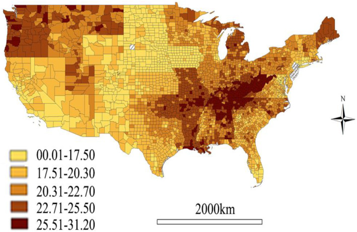
Spatial distribution of the prevalence of depression by county.
Population density varies widely among US counties (Figure 4). Except for some counties in New York, Chicago, and Los Angeles, etc., the vast majority of counties have relatively low population density. Population clustering and job clustering occur more frequently in the eastern US with limited land rather than the western portion. Levels of land mixed use and job mixed layout are high in north‐central US, which tends to have lower depression rates. The distribution of jobs‐housing balance is very similar to that of land mixed use and job mixed layout.
Figure 4.

Spatial distribution of built environment factors.
More urbanization, dense population and developed industries fill much of the eastern US, which has very limited green space and higher PM2.5 concentrations (Figure 5). It should be noted that increasing awareness of the effects of green spaces on mental health stems from concerns about declining green space due to urbanization (Byomkesh et al., 2012). Thus, green space is usually defined as urban vegetated space such as parks, grasslands, sports and playing fields and near‐road trees, rather than agricultural land (Vanaken & Danckaerts, 2018). Thus, the green space index in our study refers to the percentage of vegetated land within a census tract, including developed open space, grass, shrub, and forest areas, and excluding those areas for intensive agricultural uses. Thus, it more appropriately represents green space in urban areas rather than rural areas. Counties along the Appalachian Mountains, the west bank of the Mississippi River, and the western region of the US have higher CO concentrations. Precipitation is significantly higher in counties along the Pacific coast and in some southeastern states such as Florida and Alabama.
Figure 5.

Spatial distribution of natural environmental factors.
3.2. Built and Natural Environmental Attributes as Predictors of Depression Prevalence
The above mapping analysis provides basis for conducting more rigorous modeling, and we ran a series of regression models to identify place‐based predictors of county depression prevalence rates. Model 1 to Model 4 in Table 2 shows that built environment accounts for 17.7% of the variance in depression rates, and the addition of natural environment increases the R 2 to 28.7%. The built and natural environments explain between one‐fourth and one‐third of depression.
When all control variables are added, job sprawl, land mixed use, job mixed layout and urban areas are significantly associated with depression prevalence (Model 4). Lower values for job sprawl indices indicate greater sprawl or less compact development, thus job sprawl is linked to decreased depression prevalence. Counties with high level of land mixed use and job mixed layout, as well as urban areas are associated to lower depression prevalence. For natural environment, all variables show the same association as our hypotheses. More green spaces, lower level of air pollution, and less precipitation are linked to lower depression prevalence.
For control variables, high proportion of female, divorced people, and non‐Hispanic whites, as well as more single‐parents families share, are associated with high depression rates, while large share of aging people is usually tied to lower risk of being depression. Counties with high unemployment rate, poor access to store, more uninsured population share, and severe income segmentation are connected to more depression prevalence, while increased social capital is linked to better mental health.
We maintain that the relationship between natural environment and mental health also depends on the characteristics of built environment. Therefore, we also examine its interaction with the urban context. The coefficient of Urban*Greenspace in Model 5 is negatively significant, implying that the negative correlation between green space and depression prevalence mainly concentrates in urban areas.
3.3. Spatial Heterogeneity of Determinants of Depression
We explore the spatial heterogeneity of the relationship between depression and independent variables by using GWR. The positive and negative ratios are used to measure how these factors have different effects on depression across counties (Table 3). The positive ratio is the proportion of counties with a positive impact on depression (i.e., increasing the depression rate), while the negative ratio is the share of the counties with a negative effect on depression (i.e., decreasing the depression rate). The largest positive ratio for built and natural environment variables is 63.76% (Sprawl_P), followed by 62.66% (Sprawl_J), meaning that urban sprawl increases depression rates in more than 60% of counties. The largest negative ratio is Mixed_Land (62.89%), followed by Green_S (61.54%), indicating that mixed land use and green space decrease depression risks in more than 60% of counties. Thus, the associations between built and natural environments and depression are unevenly distributed across counties. Conversely, there are some demographic and SES factors are spatially stationary. Specifically, for more than 80% counties, high female share, more non‐Hispanic white population, less aging people, single‐parent family structure and income segregation are associated with higher depression prevalence.
Table 3.
Summary of GWR Coefficient Estimates at County Level
| Min. | Median | Max. | Global | Positive ratio (%) | Negative ratio (%) | |
|---|---|---|---|---|---|---|
| Sprawl_J | −1.983 | 0.161 | 1.565 | 0.316 | 62.66 | 37.34 |
| Sprawl_P | −1.321 | 0.075 | 2.023 | 0.074 | 63.76 | 36.24 |
| Mixed_Land | −55.202 | −1.521 | 8.444 | −4.707 | 37.11 | 62.89 |
| Mixed_Job | −14.087 | −0.610 | 32.266 | −2.587 | 43.64 | 56.36 |
| Balance_JH | −9.318 | 0.581 | 42.082 | −0.260 | 59.64 | 40.36 |
| Density_P | −2.472 | −0.030 | 3.737 | −0.055 | 47.83 | 52.17 |
| Urban | −2.882 | 0.056 | 3.552 | −0.529 | 52.40 | 47.60 |
| Green_S | −14.633 | −0.638 | 10.298 | 0.022 | 38.46 | 61.54 |
| PM2.5 | −1.997 | −0.027 | 1.060 | 0.196 | 43.42 | 56.58 |
| CO | −42.116 | 0.829 | 32.446 | 2.462 | 57.52 | 42.48 |
| Precipitation | −2.600 | 0.139 | 3.870 | 0.251 | 63.69 | 36.31 |
| Gender | −194.910 | 10.621 | 75.944 | 12.971 | 89.25 | 10.75 |
| Aging | −52.404 | −9.846 | 22.827 | −18.382 | 15.96 | 84.04 |
| Divorce_R | −148.120 | 7.199 | 83.707 | 23.034 | 65.59 | 34.41 |
| Racial_C | −1.955 | −0.141 | 1.819 | −0.273 | 39.81 | 60.19 |
| Family_S | −8.951 | 9.246 | 45.233 | 15.178 | 94.53 | 5.47 |
| Social_C | −3.940 | 2.858 | 21.289 | 6.329 | 82.75 | 17.25 |
| Growth_J | −84.316 | −5.869 | 197.080 | −3.052 | 33.22 | 66.78 |
| Rate_Unemp | −1.064 | 0.062 | 0.538 | 0.157 | 73.87 | 26.13 |
| Store_A | −16.051 | 1.212 | 114.100 | 4.292 | 63.82 | 36.18 |
| Uninsured_P | −0.329 | 0.080 | 1.263 | 0.173 | 68.97 | 31.03 |
| Income_S | −21.860 | 7.069 | 34.576 | 8.387 | 84.62 | 15.38 |
We further the above analysis by mapping the correlations of population density and social capital and depression rates, which shows more significant spatial patterns than other variables. Although high population density is linked to less depression prevalence in the vast majority of counties, it shows positive ties with depression risk in a few northeastern metropolitan areas such as the New York and Philadelphia‐Camden‐Wilmington Metropolitan Areas (Figure 6). Although the positive coefficients are also concentrated in Minneapolis–Saint Paul and Salt Lake City metropolitan areas, the P‐value in these regions are larger than 0.1, that is, the coefficients are insignificant in these regions. Thus, we cannot conclude the relationship between population density and depression rates is positive in these regions. Different from the majority of counties, high level of social capital is associated with high depression prevalence in northwestern counties and some counties in the northeastern region (Figure 7). Although some north‐central counties show the positive relationship between social capital and depression rates, only coefficients for counties in south Minnesota are significant.
Figure 6.

Effects of population density on depression.
Figure 7.

Effects of social capital on depression.
3.4. Determinants of Depression in Northwestern and Southeastern Counties
There are two main high depression prevalence regions in US, that is, northwestern and southeastern counties (Figure 2), which need further examination. Model 1 to Model4 in Table 4 show the multiple linear regression results for northwestern counties. Correlation analysis for northwestern counties shows that there is a high correlation between land mixed use, job mixed layout and jobs‐housing balance, which differs from findings based on counties nationwide. Considering high land mixed use tends to have more job mixed layout and high level of jobs‐housing balance, we only include land mixed use in our regression. To avoid inaccurate estimation caused by omitted variables, we also included the mean value of three variables (Mixed index) in the regression in Model 5. Table 5 shows the regression results for southeastern counties.
Table 4.
Determinants of Depression in Northwestern Counties
| Variables | Model 1 | Model 2 | Model 3 | Model 4 | Model 5 | |
|---|---|---|---|---|---|---|
| Dep | Dep | Dep | Dep | Dep | ||
| Built Environment | Sprawl_J | −0.411* (0.212) | −0.279 (0.200) | −0.216 (0.189) | −0.168 (0.176) | −0.166 (0.178) |
| Sprawl_P | 0.120 (0.199) | −0.0439 (0.184) | −0.116 (0.173) | −0.0506 (0.165) | −0.0408 (0.170) | |
| Mixed_Land | −8.496*** (2.264) | −6.755*** (2.214) | −5.602** (2.192) | −0.0512 (1.875) | ||
| Mixed Index | 0.380 (2.230) | |||||
| Density_P | 0.171 (0.217) | −0.0522 (0.236) | −0.134 (0.228) | −0.343 (0.274) | −0.354 (0.277) | |
| Urban | 0.136 (0.258) | 0.0366 (0.256) | −0.0384 (0.258) | 0.182 (0.227) | 0.193 (0.217) | |
| Natural Environment | Green_S | −1.270 (1.037) | −1.223 (0.992) | −1.579* (0.805) | −1.595** (0.805) | |
| PM2.5 | 0.270* (0.139) | 0.171 (0.143) | 0.117 (0.145) | 0.115 (0.145) | ||
| CO | 7.333* (4.015) | 5.789 (3.930) | 3.171 (3.378) | 3.172 (3.376) | ||
| Precipitation | 0.121*** (0.0258) | 0.0923*** (0.0272) | 0.0567* (0.0300) | 0.0569* (0.0295) | ||
| Individual (or demographic) Factors | Gender | 28.32*** (7.326) | 14.78** (6.404) | 14.76** (6.330) | ||
| Aging | −5.479 (3.756) | −5.558 (4.831) | −5.586 (4.780) | |||
| Divorce_R | 0.0307*** (0.0111) | 0.0328*** (0.0107) | 0.0332*** (0.0106) | |||
| Race_C | 0.856 (1.286) | −0.709 (1.264) | −0.737 (1.313) | |||
| Family_S | 4.907*** (1.859) | 3.228* (1.875) | 3.279* (1.854) | |||
| Socioeconomic Conditions | Social_C | −0.312** (0.148) | −0.324** (0.148) | |||
| Growth_J | 0.986 (9.705) | 0.820 (9.676) | ||||
| Rate_Unemp | 0.118** (0.0453) | 0.118** (0.0453) | ||||
| Store_A | 1.796 (1.306) | 1.798 (1.305) | ||||
| Uninsured_P | −0.186*** (0.0317) | −0.188*** (0.0326) | ||||
| Income_S | 6.210* (3.611) | 6.251* (3.575) | ||||
| Crime_R | 2.64e−05 (0.00111) | 4.82e−05 (0.00110) | ||||
| Constant | 28.59*** (1.585) | 24.84*** (2.007) | 9.929** (4.357) | 15.61*** (4.547) | 15.41*** (4.529) | |
| Observations | 167 | 167 | 167 | 162 | 162 | |
| R‐squared | 0.170 | 0.263 | 0.352 | 0.557 | 0.557 | |
| VIF | 1.51 | 1.6 | 1.56 | 2.16 | 2.19 |
Note. Robust standard errors in parentheses. ***p < 0.01, **p < 0.05, *p < 0.1.
Table 5.
Determinants of Depression in Southeastern Counties
| Variables | Model 1 | Model 2 | Model 3 | Model 4 | |
|---|---|---|---|---|---|
| Dep | Dep | Dep | Dep | ||
| Built Environment | Sprawl_J | 0.624*** (0.140) | 0.575*** (0.129) | 0.370*** (0.105) | 0.174 (0.116) |
| Sprawl_P | 0.256** (0.106) | 0.102 (0.0922) | 0.147* (0.0816) | −0.0141 (0.101) | |
| Mixed_Land | −14.37*** (1.313) | −12.07*** (1.160) | −8.164*** (1.035) | −4.126*** (1.325) | |
| Mixed_Job | 0.406 (0.841) | 0.625 (0.729) | −2.472*** (0.768) | 0.439 (0.628) | |
| Balance_JH | 1.814** (0.915) | 2.135** (0.831) | 0.766 (0.644) | −0.556 (0.824) | |
| Density_P | −0.479*** (0.0857) | −0.677*** (0.109) | −0.373*** (0.0809) | −1.660*** (0.393) | |
| Urban | −0.532*** (0.134) | −0.939*** (0.123) | −0.865*** (0.106) | −0.546*** (0.108) | |
| Natural Environment | Green_S | −3.666*** (0.304) | −0.955*** (0.288) | −0.693** (0.319) | |
| PM2.5 | 0.321*** (0.0381) | 0.0608* (0.0354) | 0.0713* (0.0367) | ||
| CO | 13.07*** (1.296) | 5.852*** (1.218) | 3.626** (1.419) | ||
| Precipitation | 0.235*** (0.0301) | 0.316*** (0.0282) | 0.155*** (0.0368) | ||
| Individual (or demographic) Factors | Gender | 11.56*** (2.052) | 14.85*** (2.295) | ||
| Aging | −14.93*** (1.788) | −13.81*** (2.954) | |||
| Divorce_R | 0.00825 (0.0219) | 0.0132 (0.0139) | |||
| Race_C | 9.554*** (0.424) | 9.695*** (0.521) | |||
| Family_S | 6.664*** (0.771) | 1.212 (0.817) | |||
| Socioeconomic Conditions | Social_C | −0.663*** (0.216) | |||
| Growth_J | −7.096* (4.113) | ||||
| Rate_Unemp | 0.102*** (0.0192) | ||||
| Store_A | 3.457*** (0.827) | ||||
| Uninsured_P | −0.0349** (0.0154) | ||||
| Income_S | 15.00*** (1.662) | ||||
| Crime_R | 0.000769*** (0.000246) | ||||
| Constant | 28.11*** (0.735) | 21.36*** (0.818) | 11.55*** (1.159) | 2.331 (1.634) | |
| Observations | 2,043 | 2,042 | 2,042 | 1,672 | |
| R‐squared | 0.167 | 0.322 | 0.509 | 0.587 | |
| VIF | 1.42 | 1.47 | 1.60 | 1.89 |
Note. Robust standard errors in parentheses. ***p < 0.01, **p < 0.05, *p < 0.1.
After adding all variables, we find that there are fewer variables associated with depression prevalence in northwestern counties. No built environment variable shows significant correlation with depression prevalence (Model 4). Among other variables, socioeconomic variables have made the greatest contribution to R 2, followed by natural environment. This means socioeconomic conditions and natural environment are the main determinants of depression risks in this region. For southeastern counties, demographic variables are most relevant to the high depression rates, with the highest increased R 2. The built environment variables also make a significant contribution to R 2, thus ranking as the second most important predictors.
4. Discussion
There is the high depression prevalence clustering in US northwestern region and US southeastern and midwestern regions, while low depression prevalence mainly clustering in central United States. Compared with other regions, the northwestern regions usually have longer‐term gray and rainy weather. Less exposure to sunlight can lead to seasonal affective disorder, a subtype of depression. Southeastern regions like in the Appalachian and Southern Mississippi Valley regions, face many problems such as high poverty rates, limited employment opportunities, and generally more challenging socioeconomic conditions. People in the Great Lakes region and Maine, with cold winter temperature, also suffer more severe depression. Counties in central United States have dry and mild climate, and the adequate sunlight exposure may reduce the risk of depression. There are more rural counties in the central region. Compared to urban counties, rural counties experience fewer social disparities, less pollution, and more connection with the nature, which contribute to higher levels of mental health (Ventriglio et al., 2021).
Job sprawl may result in more open space in urban centers and more job opportunities in suburbs, which can relax people's commute and improve mental health (Garrido‐Cumbrera et al., 2018). Land mixed use areas have more access to resources, services and entertainments, which can meet residents' needs and promote more outdoor activities and social interactions (Wu et al., 2016), thereby improving mental health. Job mixed layout enables people to find jobs that interest them, preventing the sense of monotony and boredom and thus reducing risks of being depressed. The more advanced infrastructure and comprehensive healthcare in urban areas enhance people's life satisfaction, therefore urban areas are significantly correlated with good mental health. For natural environment factors, green space is linked to lower depression prevalence by absorbing airborne pollutants and making people feel relaxed (Leslie & Cerin, 2008). Due to the higher population density, more crowded public space, and more serious air pollution caused by transportation and/or industrial production in urban areas, the role of green space is more evident in urban areas. Exposure to PM2.5 and CO pollution increases the risk of depression (F. Chen et al., 2023; Liu et al., 2018; Von Lindern et al., 2016). Also, precipitation increases the potential for depression, since it reduces the time people can expose to sunlight and outdoor activities, thereby inhibiting serotonin production (Kent et al., 2009). All significant control variables support our hypotheses in Table 1, except for racial composition. Although some argue that Black/African Americans suffer more mental problems (Barnes & Bates, 2017), LaVeist et al. (2014) find that non‐Hispanic whites experience depression more than other racial/ethnic groups, which is supported by our result.
Our study also reveals significant spatial heterogeneity in the association between population density and depression, as well as social capital and depression. Different from the majority of counties, high population density is associated to higher depression prevalence in some northeastern metropolitan areas such as the New York and Philadelphia‐Camden‐Wilmington Metropolitan Areas. These metropolitan areas are characterized by high population density and limited urban space, which leads to the diseconomies of agglomeration, such as traffic jam, high housing cost, and high crime rates. Northeastern counties and some counties in the northwestern region, as well as counties in south Minnesota, show a different correlation between social capital levels and depression prevalence compared to the majority of counties. Residents in northeastern counties witness large gaps in income levels and employment opportunities, with high concentration of highly paid financial and high‐tech jobs. Dense population and intense competition may cause social stress, resulting negative effect of social capital on mental health. For example, the busy lifestyle and high competition in the New York metropolitan area are very likely to make socializing a form of pressure for some people, thus higher levels of social capital are connected with more depression risks. Counties in the northwestern region may have relatively less dense population distribution and have more significant agriculture and manufacturing industries. Increasing social capital may threaten their rural life style and likely causes more depression. Another possible reason is that since the northwest regions have higher depression rates, the depressed people may increase their social interactions to cope with their problem (De Silva et al., 2007). Counties in south Minnesota show the positive relationship between social capital and depression rates. People in these counties face more crime rates and higher income segregation, and higher social capital levels may expose them to more crimes and result in more mental stress.
When the determinants of depression in the northwestern and southeastern counties were further examined, socioeconomic conditions, followed by natural environment factors, play important roles in depression prevalence in northwestern counties, while the role of built environment is insignificant. Northwestern counties, which may be because low density rural counties account for a large proportion of northwestern counties, thus depression prevalence is less associated with built environment. Large income segregation is significant and increases people's psychological stress and mental problems. Although Washington and Oregon are known for their high‐tech industry, there are still many counties focusing on agriculture and/or forestry. Counties in some states such as Idaho and Montana are predominantly agricultural, and seasonal unemployment may be a key factor of high depression prevalence. For natural environment, precipitation is associated with high depression rates. Located in a high latitude region, northwestern counties usually go through longer overcast and rainy weather than counties in other regions. High precipitation reduces sunlight and outdoor activities and is a main determinant of depression. US Census Bureau's Household Pulse Surveys in December 2020 and January 2023 report that Seattle is among the 15 largest metro areas with the highest share of adults feeling down, depressed or hopeless.
For southeastern US counties, the high depression prevalence may be derived from demographic factors, then followed by built environment factors. Southeastern US counties have high racial disparities, unemployment rates and poverty segregation, which have brought socioeconomic problems to the region. Study finds that the hopefulness for the future can serve as a safeguard against people from the detrimental impact of adverse ones (Lankarani & Assari, 2017). Compared with African American, non‐Hispanic whites usually have less confidence in the future (Bailey et al., 2019). Thus, counties with high proportion of non‐Hispanic whites are positively linked to high depression rates. The same as the regression based on all US counties, high female and less aging people proportions are positively connected to high depression risk. The role of built environment is also important. The efficient and proper utilization of land is conducive to leaving more space for leisure and relaxation and relieving the stress of residents. Counties with more land mixed use, higher population density and more urban area are associated with less depression disorders.
Different from the regression result based on all US counties (Model 4 in Table 2), we find some socioeconomic conditions, that is, job growth and crime, only affect depression prevalence in the southeastern counties. As the region with prominent socioeconomic problems, people living there may suffer from high social stress, violence and crime, which increasing their risk of being depressed. The increased job growth rates provide employment opportunities for the unemployed and alleviate socioeconomic problems such as poverty and income segmentation, which reduces people's life pressure. Thus, both high job growth rates and decreased crime rates reduce depression rates. Last, all other significant variables have the same effect with the regression results based on all US counties, except for the proportion of uninsured people. The high association between high proportion of uninsured people and less depression may be because southeastern counties concentrate the majority of African Americans with high share of adults without health insurance (Sood & Sood, 2021).
5. Conclusion and Limitation
5.1. Conclusion
Our study identifies important variables that may impact mental health across US counties, with the built environment emerging as a significant factor. Urban sprawl is a prominent phenomenon in the US and is widely recognized as a contributor to various urban problems. It has long been associated with increased anxiety and depression, leading to negative impact on mental health (Garrido‐Cumbrera et al., 2018). However, our study reveals that job sprawl is linked to lower depression prevalence, potentially due to increased access to job opportunities and open space. Land mixed use reduces commuting and life stress. Additionally, job mixed layouts offer a more diverse range of job opportunities, increasing the likelihood of securing satisfying employment and lowering the risk of long‐term unemployment. Thus, these factors exhibit positive associations with overall mental well‐being.
It is important to acknowledge that urban sprawl may still contribute to anxiety and depression such as increasing commuting distances (Garrido‐Cumbrera et al., 2018). It is crucial to determine the extent to which job sprawl can effectively reduce depression prevalence. Implementing measures such as promoting mixed land use and diverse job layouts can help alleviate the prevalence of depression.
The natural environment is also connected with mental health. We found that the presence of green space is associated with lower depression prevalence, and this connection is particularly significant in urban areas. Increasing green space within urban areas, fostering social connections, expanding employment opportunities, and improving social security and welfare systems play significant roles in mitigating depression prevalence. As expected, PM2.5 and CO pollution worsen mental health problems. Air pollution not only induces negative moods but also poses a threat to physical health. Consequently, exposure to PM2.5 and CO is negatively correlated with overall mental well‐being. Furthermore, our findings indicate that increased precipitation is linked to a higher prevalence of depression.
The presence of social capital, which provides individuals with additional resources and robust social support (Thoits, 2011), is linked to a lower prevalence of mental disorders. However, increasing social capital may also increase peoples' stress in certain geographical contexts. Unemployment, high income segregation, limited store access and insufficient insurance coverage, which have plagued poorer neighborhoods for a long time, tend to exacerbate mental health problems.
Further analysis of influencing factors for the two high depression prevalence areas shows that socioeconomic conditions and natural environment play important roles in changing depression prevalence in northwestern counties. Unemployment, income segregation and precipitation are significantly associated with high depression rates. Depression tends to be further exacerbated by precipitation and seasonal unemployment in these regions. Implementing strategies such as expanding employment opportunities and offering unemployment subsidies can play a crucial role in preventing and alleviating depression. Our examination of the effects of January temperature and its interaction with precipitation on mental health revealed insignificant relationships. Consequently, the cold winter itself does not significantly contribute to increased depression, and winter activities such as skiing are popular and enjoyed in this region.
For southeastern counties, demographic factors, especially the racial composition, play significant roles in influencing depression prevalence. The built environment is also important. Land mixed use, high population density and more urban areas are linked to less mental disorders. It needs to be noted that some socioeconomic factors, mainly job growth and crime, only affect the depression risk in southeastern counties.
5.2. Strengths and Limitations
Our study constructs a more comprehensive analytical framework to explore the correlations between built and natural environments and the prevalence of depression, as well as their spatial heterogeneity. We have identified the various effects of multidimensional urban sprawl on mental health, which has rarely been studied previously. Moreover, our study has shown that not all dimensions of urban sprawl is bad to mental health. We have provided more nuanced analysis of the effect of natural environment on mental health, and that such effects also vary between urban and rural areas. We also demonstrate that the effect of social capital on mental health depends on places or local context. Further identification was conducted on the determinants of two areas (northwestern and southeastern counties) with high depression prevalence, indicating again the significance of places in the determination of mental health.
Our study also has limitations. In the aftermath of the COVID‐19 and associated lockdowns, concerns about mental health have heightened significantly, which has prompted a surge in public awareness and engagement, with more individuals actively participating in outdoor activities as a means to alleviate mental stress (Li & Wei, 2023). The pandemic has thus raised the importance of built and natural environment on mental health. Future research should consider the moderating effect of COVID‐19 epidemic on the relationship between built and natural environments and depression. Also, more efforts are need to interpret the locally varied relationships across different places.
Conflict of Interest
The authors declare no conflicts of interest relevant to this study.
Acknowledgments
Research reported in this publication was supported by the National Institute on Aging of the National Institutes of Health under Award Number R01AG080440 and the Wasatch Environmental Observatory, University of Utah. The content is solely the responsibility of the authors and does not necessarily represent the official views of the National Institutes of Health.
Wei, Y. D. , Wang, Y. , Curtis, D. S. , Shin, S. , & Wen, M. (2024). Built environment, natural environment, and mental health. GeoHealth, 8, e2024GH001047. 10.1029/2024GH001047
Data Availability Statement
All of the data we use is publicly available, see Table 1 Data Sources.
References
- Akoglu, H. (2018). User's guide to correlation coefficients. Turkish Journal of Emergency Medicine, 18(3), 91–93. 10.1016/j.tjem.2018.08.001 [DOI] [PMC free article] [PubMed] [Google Scholar]
- Almedom, A. M. (2005). Social capital and mental health: An interdisciplinary review of primary evidence. Social Science & Medicine, 61(5), 943–964. 10.1016/j.socscimed.2004.12.025 [DOI] [PubMed] [Google Scholar]
- Anselin, L. (1995). Local indicators of spatial association—LISA. Geographical Analysis, 27(2), 93–115. 10.1111/j.1538-4632.1995.tb00338.x [DOI] [Google Scholar]
- Astell‐Burt, T. , Mitchell, R. , & Hartig, T. (2014). The association between green space and mental health varies across the lifecourse. A longitudinal study. Journal of Epidemiology & Community Health, 68(6), 578–583. 10.1136/jech-2013-203767 [DOI] [PubMed] [Google Scholar]
- Bailey, R. K. , Mokonogho, J. , & Kumar, A. (2019). Racial and ethnic differences in depression: Current perspectives. Neuropsychiatric Disease and Treatment, 15, 603–609. 10.2147/ndt.s128584 [DOI] [PMC free article] [PubMed] [Google Scholar]
- Barnes, D. M. , & Bates, L. M. (2017). Do racial patterns in psychological distress shed light on the Black–White depression paradox? A systematic review. Social Psychiatry and Psychiatric Epidemiology, 52(8), 913–928. 10.1007/s00127-017-1394-9 [DOI] [PubMed] [Google Scholar]
- Behnisch, M. , Krüger, T. , & Jaeger, J. A. (2022). Rapid rise in urban sprawl: Global hotspots and trends since 1990. PLOS Sustainability and Transformation, 1(11), e0000034. 10.1371/journal.pstr.0000034 [DOI] [Google Scholar]
- Brueckner, J. K. , Thisse, J. F. , & Zenou, Y. (1999). Why is central Paris rich and downtown Detroit poor? An amenity‐based theory. European Economic Review, 43(1), 91–107. 10.1016/s0014-2921(98)00019-1 [DOI] [Google Scholar]
- Byomkesh, T. , Nakagoshi, N. , & Dewan, A. M. (2012). Urbanization and green space dynamics in Greater Dhaka, Bangladesh. Landscape and Ecological Engineering, 8(1), 45–58. 10.1007/s11355-010-0147-7 [DOI] [Google Scholar]
- Chen, F. , Zhang, X. , & Chen, Z. (2023). Air pollution and mental health: Evidence from China Health and Nutrition Survey. Journal of Asian Economics, 86, 101611. 10.1016/j.asieco.2023.101611 [DOI] [Google Scholar]
- Chen, J. , Chen, S. , & Landry, P. F. (2015). Urbanization and mental health in China: Linking the 2010 population census with a cross‐sectional survey. International Journal of Environmental Research and Public Health, 12(8), 9012–9024. 10.3390/ijerph120809012 [DOI] [PMC free article] [PubMed] [Google Scholar]
- Clifton, K. , Ewing, R. , Knaap, G. J. , & Song, Y. (2008). Quantitative analysis of urban form: A multidisciplinary review. Journal of Urbanism, 1(1), 17–45. 10.1080/17549170801903496 [DOI] [Google Scholar]
- Cuijpers, P. , Karyotaki, E. , Eckshtain, D. , Ng, M. Y. , Corteselli, K. A. , Noma, H. , et al. (2020). Psychotherapy for depression across different age groups: A systematic review and meta‐analysis. JAMA Psychiatry, 77(7), 694–702. 10.1001/jamapsychiatry.2020.0164 [DOI] [PMC free article] [PubMed] [Google Scholar]
- Curtis, D. S. , Kole, K. , Brown, B. B. , Smith, K. R. , Meeks, H. D. , & Kowaleski‐Jones, L. (2024). Social inequities in neighborhood health amenities over time in the Wasatch Front Region of Utah: Historical inequities, population selection, or differential investment? Cities, 145, 104687. 10.1016/j.cities.2023.104687 [DOI] [PMC free article] [PubMed] [Google Scholar]
- Cvetkovski, S. , Jorm, A. F. , & Mackinnon, A. J. (2019). An analysis of the mental health trajectories of university students compared to their community peers using a national longitudinal survey. Studies in Higher Education, 44(1), 185–200. 10.1080/03075079.2017.1356281 [DOI] [Google Scholar]
- Dang, Y. , Dong, G. , Chen, Y. , Jones, K. , & Zhang, W. (2019). Residential environment and subjective well‐being in Beijing. Environment and Planning B: Urban Analytics and City Science, 46(4), 648–667. 10.1177/2399808317723012 [DOI] [Google Scholar]
- De Silva, M. J. , Huttly, S. R. , Harpham, T. , & Kenward, M. G. (2007). Social capital and mental health: A comparative analysis of four low income countries. Social Science & Medicine, 64(1), 5–20. 10.1016/j.socscimed.2006.08.044 [DOI] [PubMed] [Google Scholar]
- Finkelstein, A. , Taubman, S. , Wright, B. , Bernstein, M. , Gruber, J. , Newhouse, J. P. , et al. (2012). The Oregon health insurance experiment: Evidence from the first year. Quarterly Journal of Economics, 127(3), 1057–1106. 10.1093/qje/qjs020 [DOI] [PMC free article] [PubMed] [Google Scholar]
- Garrido‐Cumbrera, M. , Ruiz, D. G. , Braçe, O. , & Lara, E. L. (2018). Exploring the association between urban sprawl and mental health. Journal of Transport & Health, 10, 381–390. 10.1016/j.jth.2018.06.006 [DOI] [Google Scholar]
- Greenlund, K. J. , Lu, H. , Wang, Y. , Matthews, K. A. , LeClercq, J. M. , Lee, B. , & Carlson, S. A. (2022). PLACES: Local data for better health. Preventing Chronic Disease, 19, 210459. 10.5888/pcd19.210459 [DOI] [PMC free article] [PubMed] [Google Scholar]
- Guan, N. , Guariglia, A. , Moore, P. , Xu, F. , & Al‐Janabi, H. (2022). Financial stress and depression in adults: A systematic review. PLoS One, 17(2), e0264041. 10.1371/journal.pone.0264041 [DOI] [PMC free article] [PubMed] [Google Scholar]
- Hawton, K. , i Comabella, C. C. , Haw, C. , & Saunders, K. (2013). Risk factors for suicide in individuals with depression: A systematic review. Journal of Affective Disorders, 147(1–3), 17–28. 10.1016/j.jad.2013.01.004 [DOI] [PubMed] [Google Scholar]
- Kent, S. T. , McClure, L. A. , Crosson, W. L. , Arnett, D. K. , Wadley, V. G. , & Sathiakumar, N. (2009). Effect of sunlight exposure on cognitive function among depressed and non‐depressed participants. Environmental Health, 8(1), 1–14. [DOI] [PMC free article] [PubMed] [Google Scholar]
- Kim, G. E. , & Kim, E. J. (2020). Factors affecting the quality of life of single mothers compared to married mothers. BMC Psychiatry, 20, 1–10. 10.1186/s12888-020-02586-0 [DOI] [PMC free article] [PubMed] [Google Scholar]
- Lankarani, M. M. , & Assari, S. (2017). Positive and negative affect more concurrent among Blacks than Whites. Behavioral Sciences, 7(3), 48. 10.3390/bs7030048 [DOI] [PMC free article] [PubMed] [Google Scholar]
- LaVeist, T. A. , Thorpe Jr, R. J. , Pierre, G. , Mance, G. A. , & Williams, D. R. (2014). The relationships among vigilant coping style, race, and depression. Journal of Social Issues, 70(2), 241–255. 10.1111/josi.12058 [DOI] [PMC free article] [PubMed] [Google Scholar]
- Leslie, E. , & Cerin, E. (2008). Are perceptions of the local environment related to neighbourhood satisfaction and mental health in adults? Preventive Medicine, 47(3), 273–278. 10.1016/j.ypmed.2008.01.014 [DOI] [PubMed] [Google Scholar]
- Li, H. , & Wei, Y. D. (2023). COVID‐19, cities and inequality. Applied Geography, 160, 103059. 10.1016/j.apgeog.2023.103059 [DOI] [PMC free article] [PubMed] [Google Scholar]
- Liu, S. , Ouyang, Z. , Chong, A. M. , & Wang, H. (2018). Neighborhood environment, residential satisfaction, and depressive symptoms among older adults in residential care homes. The International Journal of Aging and Human Development, 87(3), 268–288. 10.1177/0091415017730812 [DOI] [PubMed] [Google Scholar]
- Lorant, V. , Deliège, D. , Eaton, W. , Robert, A. , Philippot, P. , & Ansseau, M. (2003). Socioeconomic inequalities in depression: A meta‐analysis. American Journal of Epidemiology, 157(2), 98–112. 10.1093/aje/kwf182 [DOI] [PubMed] [Google Scholar]
- Mantler, A. , & Logan, A. C. (2015). Natural environments and mental health. Advances in Integrative Medicine, 2(1), 5–12. 10.1016/j.aimed.2015.03.002 [DOI] [Google Scholar]
- Marmot, M. , & Wilkinson, R. G. (2001). Psychosocial and material pathways in the relation between income and health. BMJ, 322(7296), 1233–1236. 10.1136/bmj.322.7296.1233 [DOI] [PMC free article] [PubMed] [Google Scholar]
- McCloud, T. , Kamenov, S. , Callender, C. , Lewis, G. , & Lewis, G. (2023). The association between higher education attendance and common mental health problems among young people in England: Evidence from two population‐based cohorts. The Lancet Public Health, 8(10), e811–e819. 10.1016/s2468-2667(23)00188-3 [DOI] [PMC free article] [PubMed] [Google Scholar]
- McKee‐Ryan, F. , Song, Z. , Wanberg, C. R. , & Kinicki, A. J. (2005). Psychological and physical well‐being during unemployment: A meta‐analytic study. Journal of Applied Psychology, 90(1), 53–76. 10.1037/0021-9010.90.1.53 [DOI] [PubMed] [Google Scholar]
- McLeod, D. L. (2017). Children’s exposure to environmental toxins: Socioeconomic factors and subsequent effects on mental health and function. Center for the Human Rights of Children, 13. [Google Scholar]
- Moreno‐Agostino, D. , Wu, Y. T. , Daskalopoulou, C. , Hasan, M. T. , Huisman, M. , & Prina, M. (2021). Global trends in the prevalence and incidence of depression: A systematic review and meta‐analysis. Journal of Affective Disorders, 281, 235–243. 10.1016/j.jad.2020.12.035 [DOI] [PubMed] [Google Scholar]
- Pamplin, II, J. R. , & Bates, L. M. (2021). Evaluating hypothesized explanations for the Black‐White depression paradox: A critical review of the extant evidence. Social Science & Medicine, 281, 114085. 10.1016/j.socscimed.2021.114085 [DOI] [PMC free article] [PubMed] [Google Scholar]
- Parker, G. , & Brotchie, H. (2010). Gender differences in depression. International Review of Psychiatry, 22(5), 429–436. 10.3109/09540261.2010.492391 [DOI] [PubMed] [Google Scholar]
- Piracha, A. , & Chaudhary, M. T. (2022). Urban air pollution, urban heat island and human health: A review of the literature. Sustainability, 14(15), 9234. 10.3390/su14159234 [DOI] [Google Scholar]
- Richardson, E. A. , Pearce, J. , Mitchell, R. , & Kingham, S. (2013). Role of physical activity in the relationship between urban green space and health. Public Health, 127(4), 318–324. 10.1016/j.puhe.2013.01.004 [DOI] [PubMed] [Google Scholar]
- Richardson, R. , Westley, T. , Gariépy, G. , Austin, N. , & Nandi, A. (2015). Neighborhood socioeconomic conditions and depression: A systematic review and meta‐analysis. Social Psychiatry and Psychiatric Epidemiology, 50(11), 1641–1656. 10.1007/s00127-015-1092-4 [DOI] [PubMed] [Google Scholar]
- Ross, C. E. (2017). Social causes of psychological distress. Routledge. [Google Scholar]
- Ryan, S. C. , Sugg, M. M. , Runkle, J. D. , & Thapa, B. (2024). Advancing understanding on greenspace and mental health in young people. GeoHealth, 8(3), e2023GH000959. 10.1029/2023gh000959 [DOI] [PMC free article] [PubMed] [Google Scholar]
- Silva, M. , Loureiro, A. , & Cardoso, G. (2016). Social determinants of mental health: A review of the evidence. The European Journal of Psychiatry, 30(4), 259–292. [Google Scholar]
- Sood, L. , & Sood, V. (2021). Being African American and rural: A double jeopardy from Covid‐19. The Journal of Rural Health, 37(1), 217–221. 10.1111/jrh.12459 [DOI] [PMC free article] [PubMed] [Google Scholar]
- Stier, A. J. , Schertz, K. E. , Rim, N. W. , Cardenas‐Iniguez, C. , Lahey, B. B. , Bettencourt, L. M. , & Berman, M. G. (2021). Evidence and theory for lower rates of depression in larger US urban areas. Proceedings of the National Academy of Sciences, 118(31), e2022472118. 10.1073/pnas.2022472118 [DOI] [PMC free article] [PubMed] [Google Scholar]
- Sturm, R. , & Cohen, D. (2014). Proximity to urban parks and mental health. The Journal of Mental Health Policy and Economics, 17(1), 19. [PMC free article] [PubMed] [Google Scholar]
- Thoits, P. A. (2011). Mechanisms linking social ties and support to physical and mental health. Journal of Health and Social Behavior, 52(2), 145–161. 10.1177/0022146510395592 [DOI] [PubMed] [Google Scholar]
- Tikkanen, R. , Fields, K. , Williams, R. D. , & Abrams, M. K. (2020). Mental health conditions and substance use: Comparing US needs and treatment capacity with those in other high‐income countries. The Commonwealth Fund. [Google Scholar]
- Vanaken, G. J. , & Danckaerts, M. (2018). Impact of green space exposure on children’s and adolescents’ mental health: A systematic review. International Journal of Environmental Research and Public Health, 15(12), 2668. 10.3390/ijerph15122668 [DOI] [PMC free article] [PubMed] [Google Scholar]
- Van Hooff, M. L. , & Van Hooft, E. A. (2014). Boredom at work: Proximal and distal consequences of affective work‐related boredom. Journal of Occupational Health Psychology, 19(3), 348–359. 10.1037/a0036821 [DOI] [PubMed] [Google Scholar]
- Ventriglio, A. , Torales, J. , Castaldelli‐Maia, J. M. , De Berardis, D. , & Bhugra, D. (2021). Urbanization and emerging mental health issues. CNS Spectrums, 26(1), 43–50. 10.1017/s1092852920001236 [DOI] [PubMed] [Google Scholar]
- Von Lindern, E. , Hartig, T. , & Lercher, P. (2016). Traffic‐related exposures, constrained restoration, and health in the residential context. Health & Place, 39, 92–100. 10.1016/j.healthplace.2015.12.003 [DOI] [PubMed] [Google Scholar]
- Wang, L. , Zhou, Y. , Wang, F. , Ding, L. , Love, P. E. , & Li, S. (2021). The influence of the built environment on people's mental health. Sustainable Cities and Society, 74, 103185. 10.1016/j.scs.2021.103185 [DOI] [Google Scholar]
- Wei, Y. D. , & Ewing, R. (2018). Urban expansion, sprawl and inequality. Landscape and Urban Planning, 177, 259–265. 10.1016/j.landurbplan.2018.05.021 [DOI] [Google Scholar]
- Wei, Y. D. , Xiao, W. , Medina, R. , & Tian, G. (2021). Effects of neighborhood environment, safety, and urban amenities on origins and destinations of walking behavior. Urban Geography, 42(2), 120–140. 10.1080/02723638.2019.1699731 [DOI] [Google Scholar]
- Wu, Y. T. , Prina, A. M. , Jones, A. , Barnes, L. E. , Matthews, F. E. , Brayne, C. , & CFAS, M. (2016). Land use mix and five‐year mortality in later life: Results from the Cognitive Function and Ageing Study. Health & Place, 38, 54–60. 10.1016/j.healthplace.2015.12.002 [DOI] [PMC free article] [PubMed] [Google Scholar]
Associated Data
This section collects any data citations, data availability statements, or supplementary materials included in this article.
Data Availability Statement
All of the data we use is publicly available, see Table 1 Data Sources.