Low-dose CT Reconstruction with Noise2Noise Network and Testing-Time Fine-Tuning

Abstract

Purpose:

Deep learning-based image denoising and reconstruction methods demonstrated promising performance on low-dose CT imaging in recent years. However, most existing deep learning-based low-dose CT reconstruction methods require normal-dose images for training. Sometimes such clean images do not exist such as for dynamic CT imaging or very large patients. The purpose of this work is to develop a low-dose CT image reconstruction algorithm based on deep learning which does not need clean images for training.

Methods:

In this paper, we proposed a novel reconstruction algorithm where the image prior was expressed via the Noise2Noise network, whose weights were fine-tuned along with the image during the iterative reconstruction. The Noise2Noise network built a self-consistent loss by projection data splitting and mapping the corresponding filtered backprojection (FBP) results to each other with a deep neural network. Besides, the network weights are optimized along with the image to be reconstructed under an alternating optimization scheme. In the proposed method, no clean image is needed for network training and the testing-time fine-tuning leads to optimization for each reconstruction.

Results:

We used the 2016 Low-dose CT Challenge dataset to validate the feasibility of the proposed method. We compared its performance to several existing iterative reconstruction algorithms that do not need clean training data, including total-variation, non-local mean, convolutional sparse-coding, and Noise2Noise denoising. It was demonstrated that the proposed Noise2Noise reconstruction achieved better RMSE, SSIM and texture preservation compared to the other methods. The performance is also robust against the different noise levels, hyperparameters and network structures used in the reconstruction. Furthermore, we also demonstrated that the proposed methods achieved competitive results without any pre-training of the network at all, i.e. using randomly initialized network weights during testing. The proposed iterative reconstruction algorithm also has empirical convergence with and without network pre-training.

Conclusions:

The proposed Noise2Noise reconstruction method can achieve promising image quality in low-dose CT image reconstruction. The method works both with and without pre-training, and only noisy data is required for pre-training.

I. Introduction

Low-dose computed tomography (CT) is of great research interest in recent years as one of the most efficient methods to reduce the radiation exposure received by patients¹. In low-dose CT, the noise in images increases dramatically due to larger relative statistical variation in number of photons. Besides diagnostic CT, similar high-noise situation also exists in other applications. For example, in dynamic perfusion CT and retrospectively gated cardiac CT, the photon flux must be controlled because local tissues undergo consecutively X-ray exposure^2,3. The material decomposed images of dual energy and spectral CT also suffer from high-noise problem due to the ill-conditioned decomposition process⁴. Micro-CT is also subject to relatively high noise because of limited photon flux of the X-ray source unless very long exposure time is used⁵.

Image reconstruction algorithms play an important role in improving image quality for low-dose CT. One of the most widely used conventional solutions is iterative image reconstruction with designed penalty functions that exploit prior knowledge of CT images, such as continuity, edge sparsity, etc.^6,7,8,9 Machine learning and deep learning, such as (convolutional) dictionary and deep autoencoders, has also been introduced to better model the priors^10,11,12. However, deep autoencoders require high-quality images for training; linear dictionaries need very few training images, but their performance is limited due to relatively low complexity of the model.

Deep neural networks based on supervised learning achieved promising image quality on CT image denoising and reconstruction. Instead of modeling the priors, neural networks directly map the low-quality images or sinograms to high-quality images through non-linear functions. The deep learning-based methods can be generally classified into two categories: (1) Denoising methods, where neither forward or backprojector is included in the network, such as most of the image-to-image mapping networks ^13,14,15; (2) Reconstruction methods, where forward or backprojection are included in the network, such as most of the unrolled networks^16,17,18,19 as well as iterative reconstruction with network prior^12,20. Despite of their superior performance, the supervised methods require high-quality training images which are not always available as previously mentioned. Furthermore, they require that training data and testing data are from the same domain, e.g. both are head scans preprocessed with the same parameters, which lead to extra efforts in gathering training dataset when working with new scan configurations.

This work was inspired by a few recent advances in image denoising with self-supervised learning. The Deep Image Prior was proposed for image denoising by training networks to map random noise to noisy images with early stopping²¹. Gong et al. extended the Deep Image Prior to PET reconstruction with MR prior²². However, satisfying image quality cannot be achieved without any priors. Lehtinen et al. proposed the Noise2Noise later, where the network was trained to map one noise realization of noisy images to another noise realization²³. Wu et al. applied the Noise2Noise to CT and MR image denoising by splitting measurements to reconstruct different noise realizations²⁴. The Noise2Noise was also applied to CT sinogram denoising by Yuan et al.^25,26

In this paper, we proposed a novel CT image reconstruction method with an innovative Noise2Noise-based penalty function. It is an iterative reconstruction method which considers the data fidelity rather than an image denoising method. Instead of using a network with fixed-weights, we formulate the loss function with respect to both the image to be reconstructed and the network weights. The loss function consists of two parts: data fidelity and Noise2Noise-based prior. Weighted least square between the forward projection and the measurement is used for the data fidelity. For the prior term, the projection data are split to two independent sets to reconstruct two images via filtered backprojection (FBP), followed by an encoder-decoder denoising network¹⁴ which maps the two FBP images to each other. The final image is reconstructed by considering both the data fidelity and its distance to the output of the denoising network. Since the loss is based on the Noise2Noise prior, the network does not need any clean images for training. By building the network weights into the loss function, the network can be fine-tuned for individual data. Compared to Noise2Noise denoising^23,24,25, the proposed Noise2Noise reconstruction considered data fidelity, which would greatly improve image details, which are essential for CT. The loss function was optimized by alternatively reducing the data fidelity term with separable quadratic surrogate ⁸ and the prior term with Adam algorithm²⁷. To demonstrate the feasibility of the proposed method, it was validated on the 2016 Low-dose CT Challenge dataset²⁸ and compared to other unsupervised/self-supervised methods including total variation, non-local mean, convolutional dictionary, and Noise2Noise denoising. The convergence of the proposed algorithm was also empirically analyzed.

II. Material and Methods

II.A. Related Works

II.A.1. Supervised Denoising

Supervised learning is the most widely used framework for deep learning-based low-dose CT image denosing, where the network is trained by mapping low-dose images to normal-dose ones:

$${\mathbf{\Theta }}^{*}=\underset{\mathbf{\Theta }}{\text{argmin}}\frac{1}{N}\sum _i‖f\left({\mathbf{z}}_i+{\mathbf{n}}_i;\mathbf{\Theta }\right)-{\mathbf{z}}_i‖,$$ (1)

where ${\mathbf{z}}_i$ is the ground truth of $i$th training image, ${\mathbf{n}}_i$ is the noise, $f\left(\mathbf{z};\mathbf{\Theta }\right)$ is the denoising convolutional neural network (CNN), $\mathbf{\Theta }$ is its weights, and $N$ is the total number of training samples. We will refer (1) as Noise2Clean in this paper.

II.A.2. Noise2Noise Denoising

The Noise2Noise framework uses noisy images instead of clean images when training denoising networks:

$${\mathbf{\Theta }}^{*}=\underset{\mathbf{\Theta }}{\text{argmin}}\frac{1}{N}\sum _i{‖f\left({\mathbf{z}}_i+{\mathbf{n}}_{i1};\mathbf{\Theta }\right)-\left({\mathbf{z}}_i+{\mathbf{n}}_{i2}\right)‖}_2^2,$$ (2)

where ${\mathbf{n}}_{i1}$ and ${\mathbf{n}}_{i2}$ are two realizations of noise. Compared to Noise2Clean (1), Noise2Noise uses noisy images ${\mathbf{z}}_i+{\mathbf{n}}_{i2}$ instead of clean images ${\mathbf{z}}_i$ as training labels.

As demonstrated by Lethtinen et al. and Wu et al.^23,24, the Noise2Noise training (2) is equivalent to supervised training with clean images when:

1. $N\to \infty$;

2. Conditional expectation $E\left\{{\mathbf{n}}_{i2}|{\mathbf{z}}_i\right\}=0$;

3. ${\mathbf{n}}_{i1}$ and ${\mathbf{n}}_{i2}$ are independent;

Condition 1 is the basic assumption for most deep learning algorithms. Condition 2 assumes zero-mean noise, which is satisfied by the noise in low-dose CT. Condition 3 assumes noise independence of the two noise realizations, which can be constructed via projection splitting²⁴ or Poisson thinning²⁶. The proposed method employed the projection splitting approach²⁴ to construct the independence noise realizations because of the simplicity. Detailed proof of these conditions are given in the appendix A.

There is major difference between the proposed method and the existing Noise2Noise approaches. Existing approaches use fixed CNN weights during testing but the proposed method will fine-tune the CNN weights for each testing sample. The fine-tuning is possible because such two noise realizations, ${\mathbf{z}}_i+{\mathbf{n}}_{i1}$ and ${\mathbf{z}}_i+{\mathbf{n}}_{i2}$ can be constructed from the testing image itself. As it will be demonstrated in section III., it is even possible to do testing without any pre-training, i.e. the CNN is fine-tuned with random initialization.

II.A.3. Deep Image Prior

Fine-tuning the CNN during image reconstruction is related to the Deep Image Prior-based approach^21,22. Deep Image Prior demonstrates that it is possible to use CNN to achieve unsupervised single image denoising by early stopping. Ulyanov et al. fits random noise to single noisy images and used early stopping to achieve image denoising²¹. Gong et al. fits prior CT or magnetic resonance (MR) images to positron emission tomography (PET) images and combines data fidelity to achieve image denoising and detail preservation²².

The major difference between our work and Gong’s work²² is that our Noise2Noise prior does not need any external, high-quality prior images. Furthermore, because ${\mathbf{z}}_i+{\mathbf{n}}_{i1}$ and ${\mathbf{z}}_i+{\mathbf{n}}_{i2}$ share the common structures, it is easier for the CNN to find the underlying structures and remove the noise compared to a cross-modality fitting used in Gong’s work²². Hence, the proposed Noise2Noise prior has good resistance to the overfitting problem in the Deep Image Prior.

II.A.4. Unrolled Network

Unrolled network^16,17,18 is a family of supervised learning method which combines iterative reconstruction (IR) with CNN. It unrolls IR algorithms to finite iterations and replaced the penalty term-related parts with trainable CNNs. There are several major differences between the proposed work and unrolled networks:

First, unrolled networks need clean images as training labels but the proposed method only needs low-dose data. Second, unrolled networks need the IR steps during training. However, the proposed method only needs image-based training if pre-training is desired; it can also work without any training phase. Hence, the training gradients do not need to backpropagate through the projectors, which makes the training faster and easier to implement. Last but not least, unrolled networks use fixed CNN weights during testing and the number of IR steps usually cannot be changed. But the proposed method optimizes CNN weights for each testing sample and the number of iterations is flexible as in conventional IR algorithms.

II.A.5. Regularization by Denoising

The proposed method alternates between a data fidelity step and a Noise2Noise-based denoising step, which resembles the Regularization by Denoising (RED)²⁹. However, there are major differences between RED and the proposed method. RED optimizes the image to be reconstructed with a fixed denoiser in each iteration, whereas the proposed method optimizes the image and the denoising network at the same time. As discussed in the appendix B, the comparing non-local mean prior is equivalent to a RED algorithm with non-local mean denoiser.

II.B. Proposed Noise2Noise Reconstruction

II.B.1. Noise2Noise Reconstruction

The testing-time cost function of the proposed approach is:

$$\begin{array}{l}{\mathbf{x}}^{*},{\mathbf{\Theta }}^{*}=\underset{\mathbf{x},\mathbf{\Theta }}{\text{argmin}}\frac{1}{{‖\mathbf{A}‖}_{\mathbf{w}}^2}{‖\mathbf{\text{Ax}}-\mathbf{p}‖}_{\mathbf{w}}^2\\ \hspace{1em}\hspace{1em}\hspace{1em}+\beta \gamma {‖\mathbf{x}-\frac{f\left({\mathbf{z}}_1;\mathbf{\Theta }\right)+f\left({\mathbf{z}}_2;\mathbf{\Theta }\right)}{2}‖}_2^2\\ \hspace{1em}\hspace{1em}\hspace{1em}+\frac{\beta }{2}\left({‖f\left({\mathbf{z}}_1;\mathbf{\Theta }\right)-{\mathbf{z}}_2‖}_2^2+{‖f\left({\mathbf{z}}_2;\mathbf{\Theta }\right)-{\mathbf{z}}_1‖}_2^2\right),\end{array}$$ (3)

where $\mathbf{A}$ is the system matrix, $\mathbf{x}$ is the image to be reconstructed, $\mathbf{p}$ is the projections and $\mathbf{w}$ is the noise weighting matrix. ${\mathbf{z}}_1$ and ${\mathbf{z}}_2$ are FBP images from the odd-even split projections²⁴. $f\left(\mathbf{z};\mathbf{\Theta }\right)$ is a denoising CNN with input image $\mathbf{z}$ and weights $\mathbf{\Theta }$. $\beta$ is the hyperparameter to balance between Noise2Noise prior and the data fidelity, whereas $\gamma$ is the hyperparameter to control the distance between the reconstructed image $\mathbf{x}$ and the network output. ${‖\mathbf{A}‖}_{\mathbf{w}}$ equals to $‖{\mathbf{A}}^T\mathbf{w}A‖{ }_2$ and is calculated by the power method. ${‖\mathbf{A}‖}_{\mathbf{w}}^2$ was used to bring the data fidelity loss closer to unity for easier hyperparameter tuning. ${‖\mathbf{\text{Ax}}-\mathbf{p}‖}_{\mathbf{w}}^2$ equals to ${\left(\mathbf{\text{Ax}}-\mathbf{p}\right)}^T\mathbf{w}(\mathbf{\text{Ax}}-\mathbf{p})$.

There are three terms in the cost function (3). The first term is the data fidelity between the image to be reconstructed $\mathbf{x}$ and the measurement $\mathbf{p}$. The last term is the Noise2Noise prior, which fits the two noise-independent FBP images ${\mathbf{z}}_1$ and ${\mathbf{z}}_2$ to each other. The middle term is the relaxation term, which applies soft constraints between $\mathbf{x}$ and the CNN output $f\left({\mathbf{z}}_1;\mathbf{\Theta }\right)+f\left({\mathbf{z}}_2;\mathbf{\Theta }\right)/2$. Such soft constraints make the structural preservation not solely depend on the complexity of the CNN.

Since there are two major hyperparameters $\beta$ and $\gamma$, some strategy is required for efficient hyperparameter tuning. Luckily, the second and third terms are both image-to-image distance whose values are in the same magnitude, so $\gamma$ should be in the order of 1. To tune $\beta$, $\gamma$ could be set to a relative large value such as 10 first so that $\mathbf{x}$ is almost constrained to the network’s output. Then $\gamma$ can be optimized solely or jointly with $\beta$.

A flowchart of the proposed Noise2Noise reconstruction method is given in figure 1. We observed that odd-even projection splitting would lead to systematic difference between ${\mathbf{z}}_1$ and ${\mathbf{z}}_2$ especially in rebinned data. To compensate for the bias, some randomness is added to the splitting: for projections $2l$ and $2l+1$ where $l$ is an integer, projection $2l$ is randomly assigned to the odd or even set whereas projection $2l+1$ is assigned to the other. This random split scheme would significantly reduce the structural correlation between ${\mathbf{z}}_1$ and ${\mathbf{z}}_2$ without severe artifacts in the FBP images.

Figure 1:

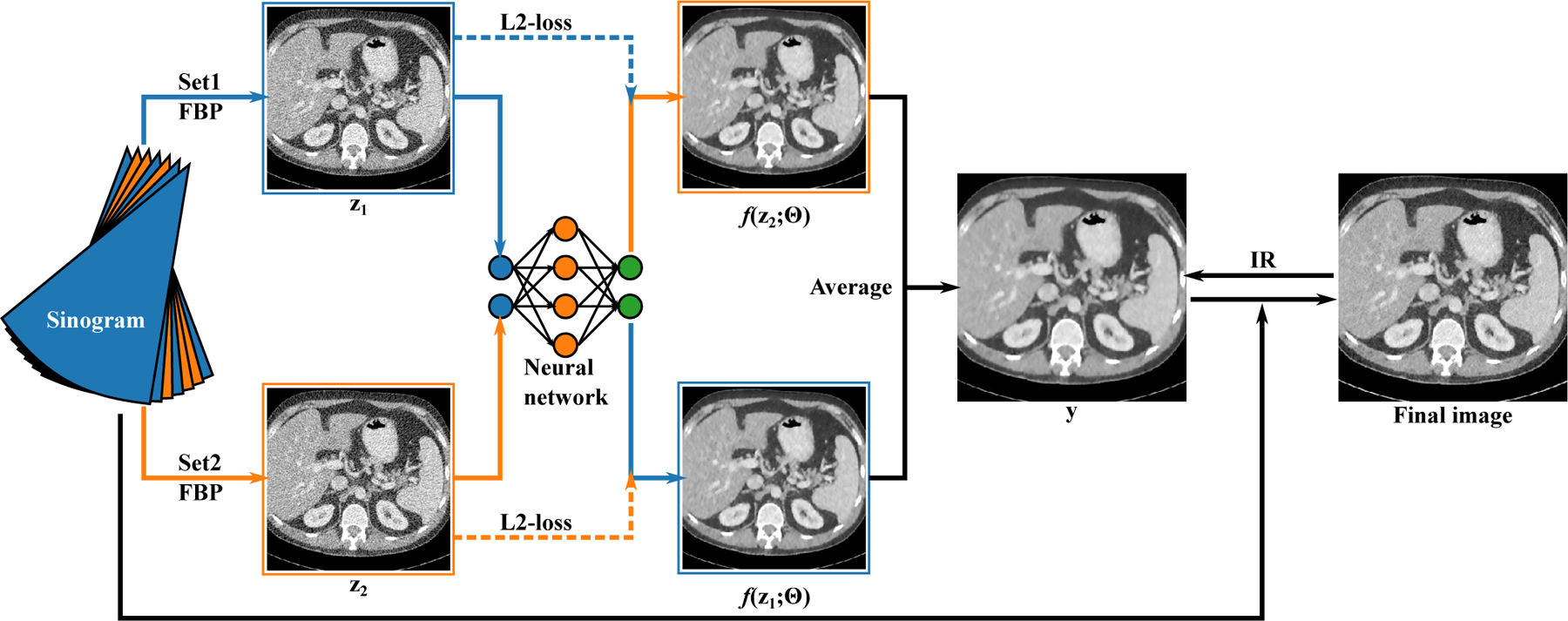
The schematic of the Noise2Noise reconstruction. The sinogram is divided into two sets (blue and orange) and reconstructed with FBP independently (${\mathbf{z}}_1$ and ${\mathbf{z}}_2$). The network tries to map ${\mathbf{z}}_1$ to ${\mathbf{z}}_2$ and vice versa. The average of the network outputs, $\mathbf{y}$, is used as a prior during the IR. The IR updates both the image to be reconstructed and the network weights.

We employed the alternating optimization strategy to reduce the cost function (3). The following two sub-problems are constructed:

$$\begin{array}{l}{g}_1\left(\mathbf{x};{\mathbf{\Theta }}^{\left(n-1\right)}\right)=\frac{1}{{‖\mathbf{A}‖}_w^2}{‖\mathbf{\text{Ax}}-\mathbf{p}‖}_{\mathbf{w}}^2\\ \hspace{1em}+\beta \gamma {‖\mathbf{x}-\frac{f\left({\mathbf{z}}_1;{\mathbf{\Theta }}^{\left(n-1\right)}\right)+f\left({\mathbf{z}}_2;{\mathbf{\Theta }}^{\left(n-1\right)}\right)}{2}‖}_2^2,\end{array}$$ (4)

$$\begin{array}{l}{g}_2\left(\mathbf{\Theta };{\mathbf{x}}^{\left(n\right)}\right)=\gamma {‖{\mathbf{x}}^{\left(n\right)}-\frac{f\left({\mathbf{z}}_1;\mathbf{\Theta }\right)+f\left({\mathbf{z}}_2;\mathbf{\Theta }\right)}{2}‖}_2^2\\ \hspace{1em}+\frac{1}{2}\left({‖f\left({\mathbf{z}}_1;\mathbf{\Theta }\right)-{\mathbf{z}}_2‖}_2^2+{‖f\left({\mathbf{z}}_2;\mathbf{\Theta }\right)-{\mathbf{z}}_1‖}_2^2\right).\end{array}$$ (5)

Denoting the original problem (3) as $g\left(\mathbf{x};\mathbf{\Theta }\right)$, $g_1$ is corresponding to the first two terms of $g$ who are related to $\mathbf{x}$ and $g_2$ is corresponding to the last two terms of $g$ who are related to $\mathbf{\Theta }$. If ${\mathbf{x}}^{\left(n\right)}$ satisfies that:

$$g_1\left({\mathbf{x}}^{\left(n\right)};{\mathbf{\Theta }}^{\left(n-1\right)}\right)<g_1\left({\mathbf{x}}^{\left(n-1\right)};{\mathbf{\Theta }}^{\left(n-1\right)}\right),$$ (6)

then

$$g\left({\mathbf{x}}^{\left(n\right)};{\mathbf{\Theta }}^{\left(n-1\right)}\right)<g\left({\mathbf{x}}^{\left(n-1\right)};{\mathbf{\Theta }}^{\left(n-1\right)}\right)$$ (7)

holds because the last term of $g$ is not related to $\mathbf{x}$.

Similarly, for ${\mathbf{\Theta }}^{\left(\mathbf{n}\right)}$ that

$$g_2\left({\mathbf{\Theta }}^{\left(n\right)};{\mathbf{x}}^{\left(n\right)}\right)<g_2\left({\mathbf{\Theta }}^{\left(n-1\right)};{\mathbf{x}}^{\left(n\right)}\right),$$ (8)

we have

$$g\left({\mathbf{x}}^{\left(n\right)};{\mathbf{\Theta }}^{\left(n\right)}\right)<g\left({\mathbf{x}}^{\left(n\right)};{\mathbf{\Theta }}^{\left(n-1\right)}\right)$$ (9)

because the first term of $g$ is not related to $\mathbf{\Theta }$. Hence, by alternatively reducing $g_1$ and $g_2$, we constructed the following sequence:

$$g\left({\mathbf{x}}^{\left(n\right)};{\mathbf{\Theta }}^{\left(n\right)}\right)<g\left({\mathbf{x}}^{\left(n\right)};{\mathbf{\Theta }}^{\left(n-1\right)}\right)<g\left({\mathbf{x}}^{\left(n-1\right)};{\mathbf{\Theta }}^{\left(n-1\right)}\right),$$ (10)

which reduces the original cost function (3).

The alternating optimization approach also decouples the original problem (3) into the image reconstruction problem (4) and the network training problem (5). Problem (4) has very simple L2 constraints and can be reduced by Separable quadratic surrogate (SQS)⁹. For problem (5), Limited memory Broyden-Fletcher-Goldfard-Shanno (L-BFGS)^30,31 with line search can be used to ensure monotone. To improve computational efficiency, we used ordered subsets (OS) and Nesterov’s acceleration³² with SQS for (4) and patch-based Adam²⁷ instead of L-BFGS for (5). Empirical convergence with these accelerations will be discussed in the results.

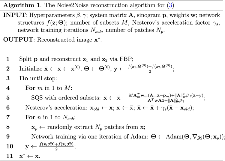
The proposed Noise2Noise reconstruction algorithm is summarized in table 1. In step 2, $\mathbf{x}$ can be initialized from FBP results or zero; $\mathbf{\Theta }$ can be pre-trained (see section II.B.2.) or randomly initialized. We used fixed number of iterations as the stopping criteria for the stopping condition in step 3. Step 4 to 6 are optimizing (4) via SQS with ordered subsets and Nesterov’s acceleration.${\mathbf{A}}_m$, ${\mathbf{w}}_m$ and ${\mathbf{p}}_m$ are the system matrix, weighting matrix, and projections corresponding to the $m$ th subset. Step 7 to 9 optimizes (5) by training the network on patches with Adam algorithm. It is important to enable patch-based network training for CT imaging due to the large size of CT images in real 3D applications.

Table 1:

The Noise2Noise Reconstruction Algorithm.

II.B.2. Pre-Training

Although algorithm in table 1 can be initialized with random weights $\mathbf{\Theta }$, pre-training with a limited number of low-dose images would lead to faster convergence of the algorithm. Pre-training is also a common technique used in dictionary learning-based CT image reconstruction^10,11. We proposed to use image-domain training²⁴ on a small number of images:

$$\begin{array}{l}{\mathbf{\Theta }}^{\left(0\right)}=\underset{\mathbf{\Theta }}{\text{argmin}}\frac{1}{N}\sum _i\frac{1}{2}{‖f\left({\mathbf{z}}_{i1};\mathbf{\Theta }\right)-{\mathbf{z}}_{i2}‖}_2^2\\ \hspace{1em}+\frac{1}{2}{‖f\left({\mathbf{z}}_{i2};\mathbf{\Theta }\right)-{\mathbf{z}}_{i1}‖}_2^2\\ \hspace{1em}+{\gamma }_d{‖\frac{f\left({\mathbf{z}}_{i1};\mathbf{\Theta }\right)+f\left({\mathbf{z}}_{i2};\mathbf{\Theta }\right)}{2}-\frac{{\mathbf{z}}_{i1}+{\mathbf{z}}_{i2}}{2}‖}_2^2,\end{array}$$ (11)

where ${\mathbf{z}}_{i1}$ and ${\mathbf{z}}_{i2}$ are the two noisy FBP images reconstructed by projection splitting of the ith noisy training image. ${\gamma }_d$ is a hyperparameter to balance between noise removal and structural preservation. Because the inputs to the denoising CNN, ${\mathbf{z}}_{i1}$ and ${\mathbf{z}}_{i2}$ have higher noise level than original noisy images, training without any constraint would generate oversmoothed results due to the excessive noise level in the source images.

II.C. Experimental Validation

II.C.1. Dataset

We employed the 2016 Low-dose CT Grand Challenge dataset²⁸ for the validation of the proposed method. The dataset contains projections from 10 patients’ abdominal scans with Siemens Somatom Definition Flash. Realistic quarter-dose projections were simulated by Mayo Clinic from the original normal-dose data³³. We rebinned the data to multi-slice fanbeam geometry³⁴ with 1mm slice thickness and took 3-layer average to form 3mm thick fanbeam sinograms for our 2D reconstruction studies. Some important geometric parameters of the 2D rebinned fanbeam are given in table 2.

Table 2:

Parameters of the Rebinned Geometry.

Parameter	Value
Slice thickness	3mm
Pixel size of image	0.8mm × 0.8mm
Resolution of image	640 × 640
Views per rotation	2304
Number of detector units	736
Pixel size of detector	1.2858mm
Source to ios-center distance	595mm
Source to detector distance	1086.5mm

We randomly extracted 10 low-dose slices from each patient for the studies, which gave 100 slices of sinograms in total. We further randomly selected 10 calibrating slices from the total 100 testing slices for any hyperparameter tuning and pre-training. The pre-trainings only engage low-dose sinograms. A larger dataset which contained 50 slices per patients was also prepared for supervised learning (Noise2Clean).

II.C.2. Parameters

In the basic configuration, we used an encoder-decoder network as shown in figure 2. It has 4 encoding modules and 4 decoding modules and shares a similar structure with UNet³⁵ but without resampling and channel-doubling. The network was pre-trained under the Noise2Noise denoising framework (2) with ${\gamma }_d=0$ on the 10 calibrating slices for 1,000 iterations to provide a better initialization. The network was trained on 96 × 96 patches with a mini-batch size of 40 by Adam algorithm with a learning rate of 10⁻³.

Figure 2:

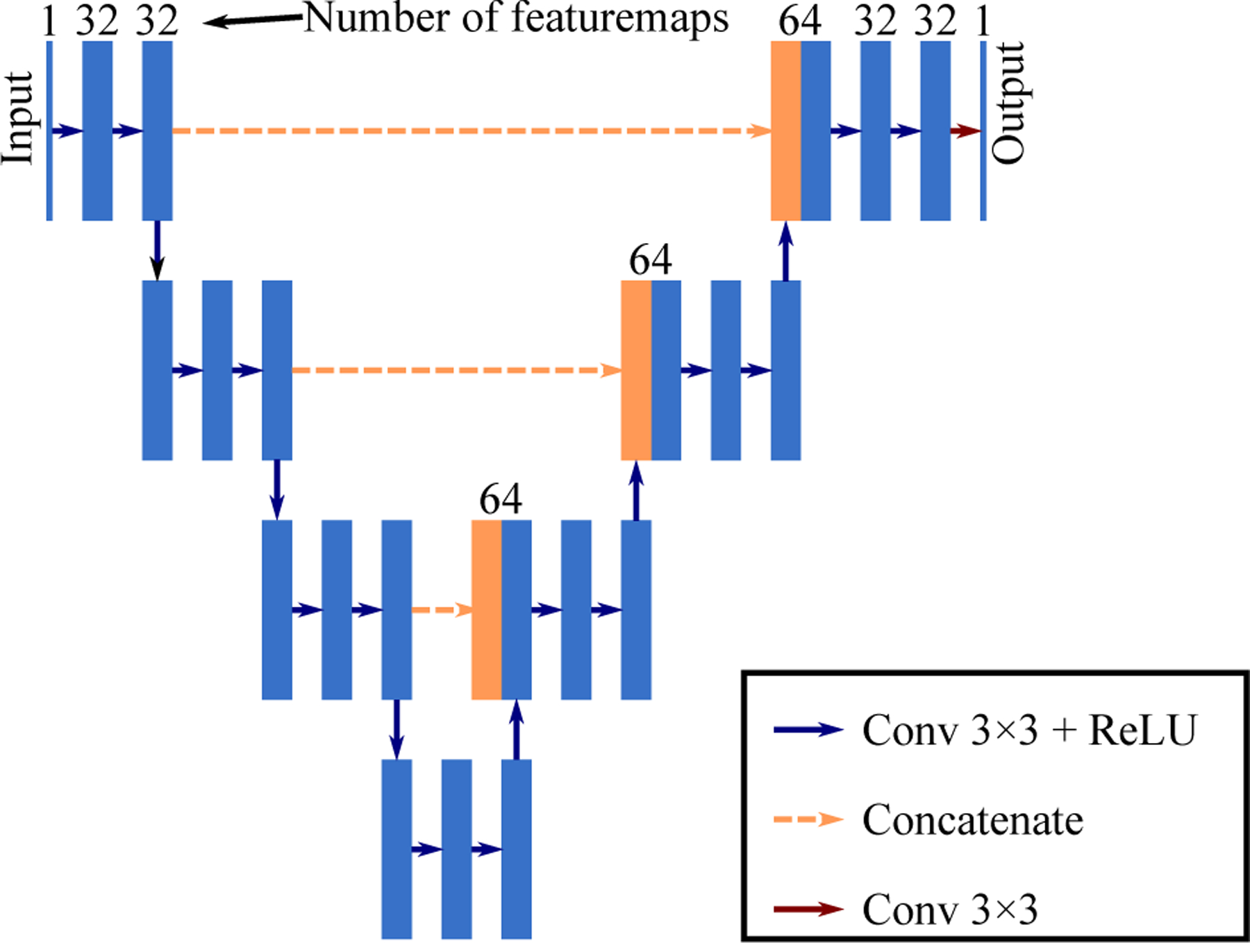
The encoder-decoder network used in the studies. The resolution remained the same for all the featuremaps in the network, which was 96 × 96 during patch-based training and 640 × 640 during inference. The number of channels for all the blue blocks were 32 except for the input and output layer.

During reconstruction, $\mathbf{x}$ was initialized by FBP. Number of subsets $M=12$. Nesterov’s acceleration factor ${\gamma }_s=0.5$. Number of network training iterations $N_{sub}=5$. In step 9 of algorithm 1, the network was fine-tuned on 40 96 × 96 patches for each iteration with Adam optimizer with learning rate of 10⁻³. The total number of outer iterations was set to 100. For quarter-dose reconstruction from Mayo’s simulation, we set $\beta =7.5\times {10}^{-4}$ and $\gamma =5$ based on root mean square error (RMSE) against the normal-dose images on the 10 calibrating slices. Distance-driven projector and backprojectors realized by CUDA on graphics processing units (GPU) were used for all the reconstructions. Tensorflow 1.11 was used for neural networks³⁶. The codes are available at https://github.com/wudufan/Noise2NoiseReconstruction.

II.C.3. Comparing Methods

We realized comparing methods including iterative reconstruction (IR) with Gaussian, total variation (TV)³⁷, spatial-encoded non-local mean (NLM)⁷ and convolutional sparse coding (CSC)¹¹ penalties. To investigate the benefit of including reconstruction, the Noise2Noise denoising ($\text{N}2{\text{N}}_d$) was also realized according to (2) using the sinogram splitting shown in Fig. 1. The Noise2Noise Reconstruction with and without pre-training will be denoted as $\text{N}2{\text{N}}_r$ and $\text{N}2{\text{N}}_r$ (w/o pre). Furthermore, an encoder-decoder network was trained by supervised learning (1) with L2-norm, i.e. Noise2Clean (N2C).

IR with Gaussian penalty was provided as the baseline method instead of FBP to eliminate the modeling error between FBP and IR. The strength of Gaussian penalty was tuned so that on normal-dose data IR achieved similar noise level with FBP with Hann filter. The same strength of penalty was used for low-dose reconstruction to visualize the noise levels. CSC was trained on the 10 calibrating low-dose FBP images with the same dictionary settings with Bao et al.¹¹

The Noise2Noise denoising was trained on the 10 calibrating slices using the following equation:

$$\begin{array}{l}{\mathbf{\Theta }}^{*}=\underset{\mathbf{\Theta }}{\text{argmin}}\frac{1}{N}\sum _i\gamma {‖\frac{{\mathbf{z}}_{i1}+{\mathbf{z}}_{i2}}{2}-\frac{f\left({\mathbf{z}}_{i1};\mathbf{\Theta }\right)+f\left({\mathbf{z}}_{i2};\mathbf{\Theta }\right)}{2}‖}_2^2\\ \hspace{1em}+\frac{1}{2}\left({‖f\left({\mathbf{z}}_{i1};\mathbf{\Theta }\right)-{\mathbf{z}}_{i2}‖}_2^2+\frac{1}{2}{‖f\left({\mathbf{z}}_{i2};\mathbf{\Theta }\right)-{\mathbf{z}}_{i1}‖}_2^2\right),\end{array}$$ (12)

where ${\mathbf{z}}_{i1}$ and ${\mathbf{z}}_{i2}$ are the two split reconstructions of the $i$th training image. To avoid model errors between IR and analytical reconstruction, we used the Gaussian baseline for ${\mathbf{z}}_{i1}$ and ${\mathbf{z}}_{i2}$ instead of FBP. The hyperparameter, $\gamma$, were tuned to for best RMSEs on the 10 training slices. During testing, the denoised images will be:

$${\mathbf{z}}_d=\frac{f\left({\mathbf{z}}_1;{\mathbf{\Theta }}^{*}\right)+f\left({\mathbf{z}}_2;{\mathbf{\Theta }}^{*}\right)}{2},$$ (13)

where ${\mathbf{z}}_1$ and ${\mathbf{z}}_2$ are reconstructed using the baseline IR with Gaussian prior.

The encoder-decoder network used in the Noise2Clean has the same structure in figure 2. The network was trained on a larger dataset which contained 50 slices per patients. The training was done by Adam algorithm with learning rate of 10⁻³ for 100 epochs. Five-fold cross validation was used to evaluate the method, where in each fold 8 patients was used for training and the rest 2 patients for testing. The total testing results was the aggregation of the testing slices from all the 5 folds. The final evaluation was done on the testing slices that were the same with the 100 testing slices used in the other studies.

For comparison, we calculated RMSEs and structural similarity indices (SSIM)³⁸ against the normal-dose reference images on the central 384 × 384 pixels. The SSIM were calculated in the soft tissue window (40 ± 400 HU) to reflect perceptual difference in the corresponding window.

II.C.4. Study Designs

The studies mainly contain four parts: comparing study on the quarter-dose projections simulated by Mayo, hyperparameter study, multi-dose-level study, and convergence study.

In the comparing study, the hyperparameters of all the unsupervised methods were optimized for RMSE based on the 10 calibrating slices. Then they were applied to all the 100 slices to compare RMSE, SSIM and visual image quality. For Noise2Clean, 5-fold cross validation was used. In each fold, 8 patients’ data were used for training, and the CNN was tested on the other 2 patients on the same slices with the unsupervised methods. The final results for Noise2Clean was aggregated from all the testing sets in the 5 folds.

For the hyperparameter study, we extensively studied the influence of parameters to the Noise2Noise reconstruction by tuning parameters based on the baseline configuration given in section II.C.2.. To save computational time, the study was only done on the 10 calibrating slices. A joint grid search was performed for $\beta$ and $\gamma$ to depict the influence of these two most important parameters. The depth of network, structures of network, and number of sub-iterations $N_{sub}$ were also explored respectively. The investigated network structures included encoder-decoder, UNet and ResNet, where UNet had the same depth with the encoder-decoder, and ResNet had similar number of trainable parameters with the encoder-decoder network.

In the multi-dose-level study, instead of Mayo’s simulated quarter-dose projections, we used forward projection from normal-dose images reconstructed by FBP with Hann filter where we could evaluate RMSE with ground truth. Different noise level was added to the projections according to Yu et al.³³. To save computational time, this study was only done on the 10 calibrating slices. Furthermore, instead of a full parameter optimization for each dose level, we only optimized the penalty strength $\beta$ for all the methods, except for Gaussian where $\beta$ remained the same to provide a reference to the noise level.

Last but not least, a convergence study was performed on one slice from Mayo’s quarter-dose simulation. We studied the influence of reconstruction acceleration techniques, where we ran 1,000 iterations with 12 ordered subsets (OS) and Nesterov acceleration, and 10,000 iterations without them. Different network training schemes were also investigated, including Adam optimization on patch with pre-training, Adam optimization on patch without pretraining, Adam optimization on the whole image with pre-training, and L-BFGS on patch with pre-training. L-BFGS was included due to its monotonic property because of the line search and relatively high efficiency.

III. Results

III.A. Reconstruction from Quarter-dose

The RMSEs and SSIMs on the 100 slices against the reference normal-dose IR with Gaussian penalty are given in figure 3. The Noise2Noise reconstruction achieved the best RMSE (18.5 ± 3.9 HU) and SSIM in soft tissue window (0.830 ± 0.060) among all the unsupervised methods with p-values less than 0.001 under dependent t-test. Compared to Noise2Clean (RMSE = 17.5 ± 4.6 HU, SSIM = 0.822 ± 0.062), Noise2Noise reconstruction had worse RMSE but higher SSIM in the soft tissue window $\left(p\le 0.001\right)$. The worse RMSE was mainly due to the inconsistent noises between the Noise2Noise reconstruction and the reference images, whereas Noise2Clean gave relatively smoothed images which led to lower RMSE.

Figure 3:

The box plot of the RMSEs and SSIMs on the 100 testing slices. $\text{N}2{\text{N}}_{\text{d}}$ is the Noise2Noise denoising; $\text{N}2{\text{N}}_{\text{r}}$ is the Noise2Noise reconstruction; $\text{N}2{\text{N}}_{\text{r}}$(w/o pre) is the Noise2Noise reconstruction without pre-training with zero-image initialization; N2C is Noise2Clean (supervised learning). The SSIMs were calculated in the soft tissue window 40 ± 400 HU. Gaussian was used as baseline instead of FBP to eliminate the modeling bias between IR and analytical reconstruction. Compared to Noise2Noise reconstruction, Noise2Noise denoising does not fine-tune during testing.

Noticeably, the Noise2Noise reconstruction without pre-training achieved very close performance to the one with pre-training. The RMSE and SSIM of the Noise2Noise reconstruction without pre-training were 18.8 ± 3.9 HU and 0.826 ± 0.060 respectively. This result indicated that the proposed method was robust and insensitive to the initialization.

Figure 4 and 5 gave the reconstructed images of two slices. Compared to the other methods, the proposed Noise2Noise reconstruction had the most similar noise level and textures with the reference images. In figure 5, a flat region on the liver was selected to calculate the its standard deviation (std) as an indicator for noise level and texture, and Noise2Noise reconstruction achieved the closest std to the reference. It should be noted that Noise2Noise reconstruction was not particularly tuned for texture preservation. The hyperparameters for all the methods were optimized for RMSE on the 10 calibrating slices. The small lesions and vessels were also well-preserved in the results of Noise2Noise reconstruction.

Figure 4:

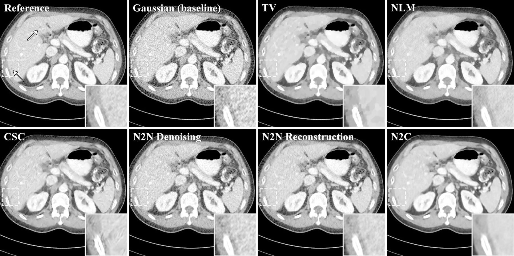
One of the reconstructed slices. Two metastases are marked by white arrows on the reference image and one of them is zoomed in. The display windows are 40 ± 400 HU. Gaussian was used as baseline instead of FBP to eliminate the modeling bias between IR and analytical reconstruction. Compared to Noise2Noise reconstruction, Noise2Noise denoising does not fine-tune for each testing image.

Figure 5:

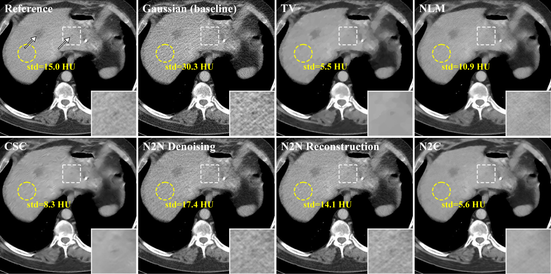
One of the reconstructed slices. Two metastases are marked by white arrows on the reference image and one of them is zoomed in. The display windows are 40 ± 400 HU. The standard deviations inside the yellow circles were also calculated. Gaussian was used as baseline instead of FBP to eliminate the modeling bias between IR and analytical reconstruction. Compared to Noise2Noise reconstruction, Noise2Noise denoising does not fine-tune for each testing image.

III.B. Influence of Hyperparameters

With baseline settings as $\beta =7.5\times {10}^{-4}$, $\gamma =5$, encoder-decoder network with 4 encoding/decoding modules (figure 2), and sub-iterations for Adam per outer iteration $N_{sub}=5$, we investigated the influence of hyperparameters for the quarter-dose reconstruction on the 10 calibrating slices and the results are given in figure 6.

Figure 6:

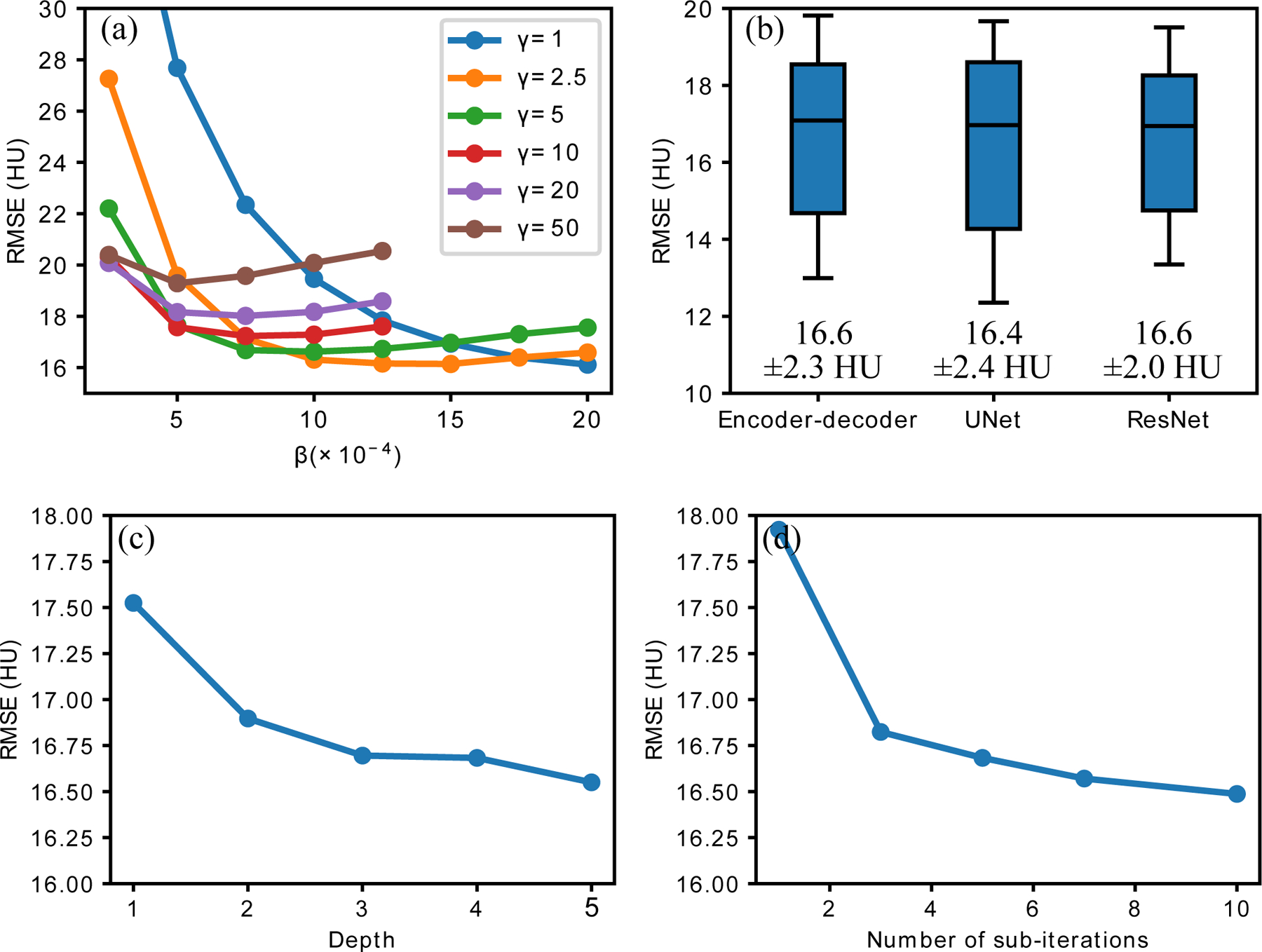
The influence of hyperparameters for quarter-dose reconstruction on the 10 calibrating slices. (a) Mean RMSEs with different $\beta$ and $\gamma$; (b) RMSEs with different network structures, UNet had same depth with encoder-decoder and ResNet had similar number of trainable parameters; (c) Mean RMSEs with different number of encoding/decoding modules; (d) Mean RMSEs with different $N_{sub}$.

Figure 6 depicted the joint influence of $\gamma$ and $\beta$ on the reconstruction results. As $\gamma$ increased, the reconstructed image $\mathbf{x}$ was more constrained to the output of the network and it led to increased insensitivity to $\beta$. On the contrary, when $\gamma$ decreased and $\mathbf{x}$ had higher freedom away from the network, the results’ sensitivity to $\beta$ increased but the peak performance would also be improved. We selected $\gamma =5$ considering both stability and peak performance in our study.

Figure 6 (b), (c) and (d) demonstrated the robustness of Noise2Noise reconstruction to different network structures and number of Adam iterations. The mean RMSEs remained almost the same for the three network structure, including encoder-decoder network, UNet and ResNet. The RMSEs changed within 1 HU when depth of network increased from 2 to 5, or number of Adam iterations changed from 3 to 10.

III.C. Multi-Noise-Level Study

In the multi-noise-level study, we inserted noise into the forward projection of normal-dose images reconstructed from FBP with Hann filter, so we had access to the ground truth images. The RMSEs on the 10 calibrating slices are given in figure 7. Reconstructed images from Gaussian, NLM, Noise2Noise and Noise2Clean are given in figure 8.

Figure 7:

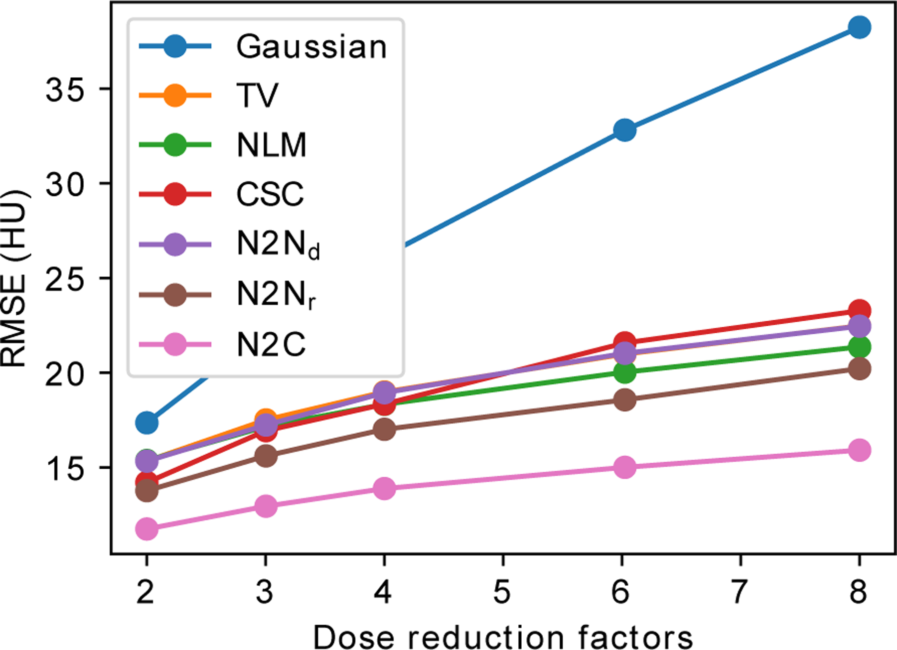
The mean RMSEs on the 10 calibrating slices for different simulated noise levels. $\text{N}2{\text{N}}_d$: Noise2Noise denoising; $\text{N}2{\text{N}}_r$: Noise2Noise reconstruction; N2C: Noise2Clean.

Figure 8:

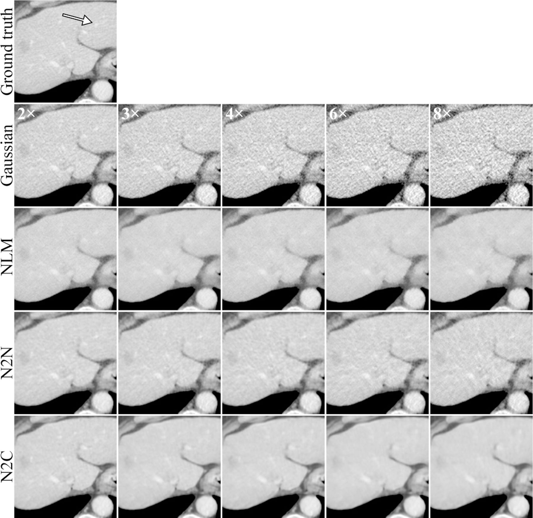
A region of interest of the reconstructed images at different dose level. The first row (Ground truth) is the full-dose reconstruction, whereas the second row and below are the results from 2, 3, 4, 6, and 8 times dose-reduction data with different methods. A vessel structure was marked by the white arrow on the ground truth image. The display windows are 40 ± 400 HU.

Figure 7 demonstrated that the proposed Noise2Noise reconstruction had consistently improved RMSEs compared to other unsupervised methods at multiple dose levels. Although Noise2Clean achieved lower RMSEs, its advantage over the Noise2Noise reconstruction did not significantly increase with reduced dose.

In figure 8, the Noise2Noise reconstruction demonstrated best texture preservation under all noise levels. It also had better structural preservation compared to NLM at the vessel marked by the white arrow. This structure was also missed by Noise2Clean, which indicated the benefits of combining iterative reconstruction and deep neural networks.

III.D. Empirical Convergence Study

The convergence curves of cost functions and RMSEs on one slice are depicted in figure 9. In terms of cost functions, all the schemes converged to approximately the same value. The algorithms converged when no acceleration was applied to reconstruction, but slowly diverged with 12 OS and Nesterov acceleration after approximately 500 iterations. The divergence was mainly due to the artifacts at the edges of field of view (FOV), because the network was applied only inside the FOV to avoid FBP’s artifacts outside FOV. The RMSEs remained stable despite of the divergence because they were calculated on the central 384 × 384 pixels which excluded the edge of FOVs.

Figure 9:

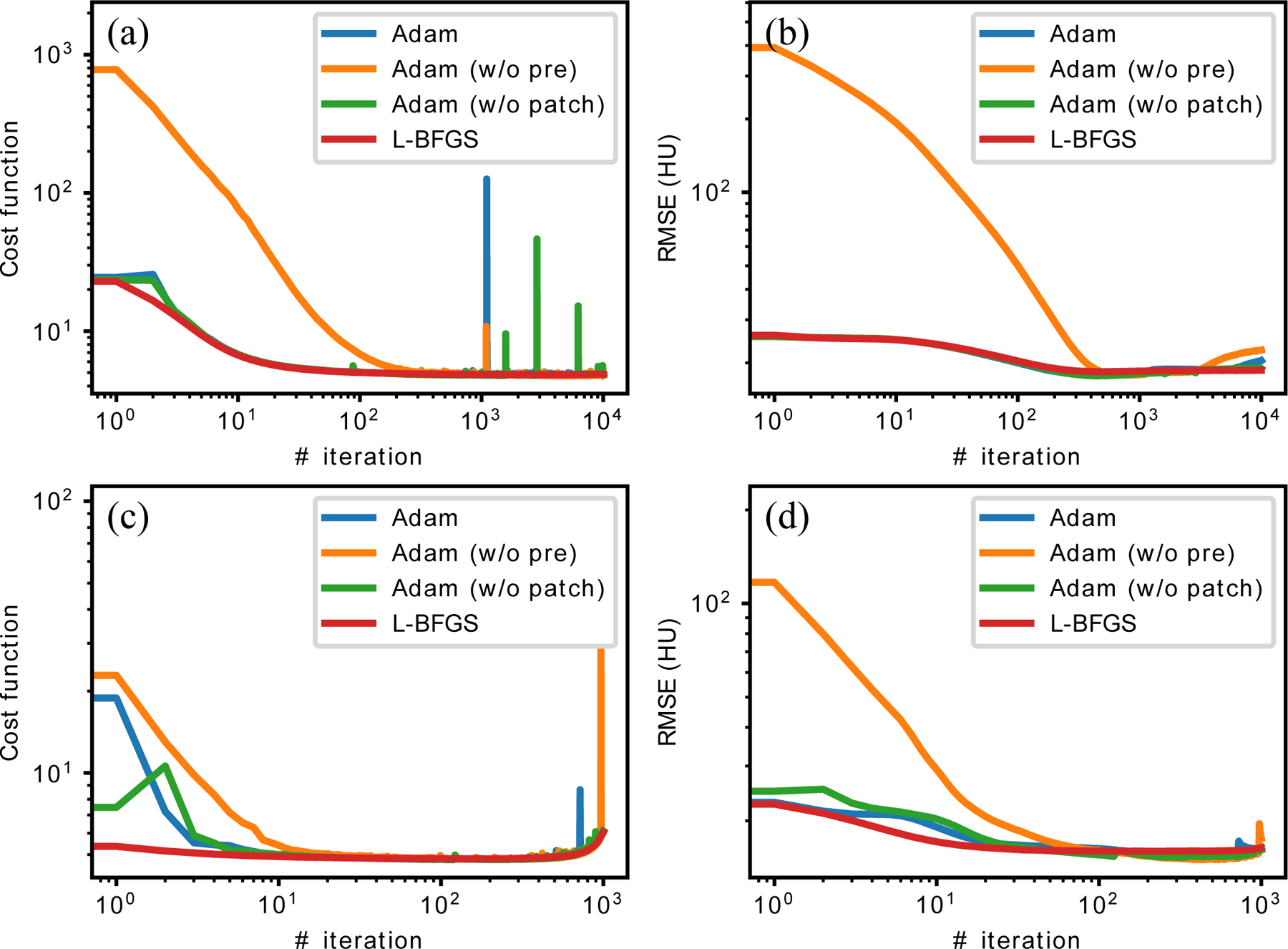
The convergence curves for one slice: (a) cost function without any OS or acceleration; (b) RMSE without any OS or acceleration; (c) cost function with 12 OS and Nesterov acceleration; (d) RMSE with 12 OS and Nesterov acceleration. Adam (w/o pre) is Adam optimization without pre-training; Adam (w/o patch) is Adam optimization on the whole image instead of patches.

Noticeably, the Noise2Noise reconstruction without any pre-training converged to the same cost function and RMSE compared to the one with pre-training, which further demonstrates that the proposed method still works even if there is no training phase.

The RMSE curves in figure 9 (b) and (d) demonstrated the methods’ resistance to the overfitting problem. There was no obvious sign for RMSE to increase in the accelerated cases or before 5,000 iterations in the unaccelerated cases. This was partially because of the relatively small number of parameters in the encoder-decoder network (≈ 148 K). However, the network was still over-parameterized and some noisy structures emerged at very late iterations as pointed by the white arrow in figure 10. Since this overfitting phenomenon only happened at very late stages, it should not be of concern for practical problems where much fewer number of iterations are used. Furthermore, this problem should also be mitigated when applied to 3D, where the images had more structures and higher dimensions.

Figure 10:

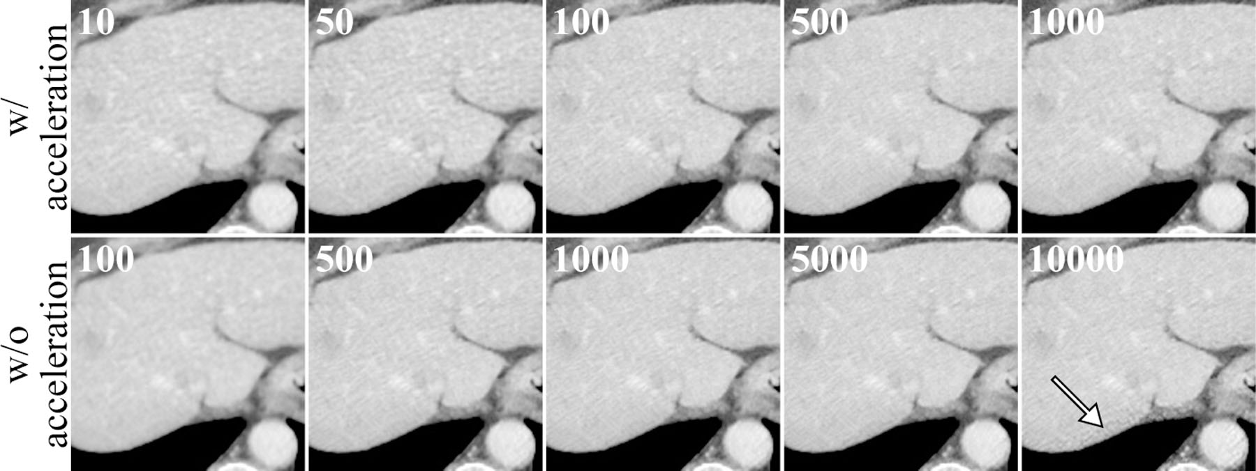
A region of interest of the reconstructed images at different iteration number. The first row is reconstruction with 12 OS and Nesterov acceleration. The second row is without OS or acceleration. The iteration numbers are displayed at the upper left corner of each image. The white arrow points to some artifacts due to overfitting of the network at very late iterations.

IV. Discussion

As shown in figure 3, the proposed Noise2Noise reconstruction (with and without pre-training) achieved the best RMSE and SSIM in the quarter-dose study among all the comparing methods except for Noise2Clean, which needs clean images as the training labels. It also achieved the best RMSE at various dose reduction rates comparing to methods except for Noise2Clean, as demonstrated in figure 7 and 8. The proposed method also has good texture preservation, as shown in 5, the Noise2Noise reconstruction has the closest noise level to the normal-dose reconstruction although it was tuned for best RMSE.

Compared to Noise2Clean, the proposed algorithm has higher noise level although the RMSE and SSIM are similar for the two methods. This is mainly because of the data fidelity term. Similar to conventional IR algorithms, the balance between the data fidelity and the prior is adjusted by the hyperparameters. Higher weight on the data fidelity term leads to noisier results, and higher weight on the prior term leads to smoother results. In the proposed method (3), there are two hyperparameters, $\beta$ and $\gamma$ to control the balance. $\beta$ is the primary parameter, which lead to smoother images with higher value. $\gamma$ is the secondary parameter which controls the distance between the reconstructed image $\mathbf{x}$ and the Noise2Noise network output. Smaller $\gamma$ will lead to noisier images, and $\gamma =0$ will render the Noise2Noise prior ineffective because $\mathbf{x}$ will be totally decoupled from the network.

One of the most significant advantage of the proposed algorithm is that it works without any pre-training as demonstrated in figure 3 and 9, where similar RMSE can be achieved with and without pre-training in later iterations. The main purpose of pre-training is to accelerate the convergence. It only requires a very small amount of noisy training data, such as 10 slices in our case, which is the same with the dictionary-based method¹¹. The low requirement on external data makes the proposed method potentially very useful for many research studies where there are very few subjects who undergo the same scan condition. The proposed method benefits from the rich representation power of deep neural networks but does not subject to the large amount of training samples.

Empirical convergence was also demonstrated as shown in figure 9 under various conditions. The convergence makes the proposed method different from most existing network-based methods, which have limited feedback from the measurement during testing time. The testing time convergence may lead to better robustness against outliers because of the feedback from the measurement.

In figure 9, some spikes presented on the loss function curves after the algorithms almost converged when Adam optimizer was used for network training. One of the most possible reasons could be that Adam used adaptive momentum that was normalized by the moving average of the network’s gradients’ magnitude. When the network was near minimum and the gradients could be close to zero, which could finally lead to very small normalization factors that cause numerical instability. This could be mitigated by more advanced algorithms such as AMSGrad³⁹. However, despite of the occasional instability of the network training, the reconstructed images $\mathbf{x}$ had soft constraint to the network output and was barely influenced by the spikes. The network restored from the spikes quickly in the following iteration. For L-BFGS, the line search process inside its sub-iterations guaranteed the algorithm’s monotonic property when no acceleration was imposed. Spikes were also not observed since L-BFGS is gradient-based.

Besides Noise2Noise, it is possible to simulate ultra-low-dose data by noise insertion to the low-dose data to train a denoising network by mapping from ultra-low-dose to low-dose. The trained network can be further applied to the low-dose data for further denoising, as demonstrated by Shocher et al. in the super-resolution tasks⁴⁰. However, the performance of the network may be sub-optimal since the training data and testing data are not in the same domain (ultra-low-dose vs. low-dose).

The proposed method does not come without weaknesses. First, we used FBP images as ${\mathbf{z}}_1$ and ${\mathbf{z}}_2$ which may be suboptimal. They can be replaced by IR results for better image quality. Second, the projection splitting approach may lead to streaking artifacts when the views are not densely sampled. Instead, Poisson thinning²⁶ can be used to generate half-dose images without angular down-sampling.

Last but not least, speed is currently the most concerned since network training is required within each iteration. In our 2D studies which were carried on a GTX 1080 Ti GPU, for each slice, SQS without OS (to minimize I/O time between CPU and GPU) required 0.22 seconds per iteration, Adam needed 0.19 seconds per network training iteration on 40 96 × 96 patches, and network inference required 0.08 seconds. Network training consumed the most time. However, since the networks are trained on patches, its relative time compared to reconstruction can be reduced when applied to 3D¹⁸, because 40 96×96×96 patches will be much sparser in 3D compared to 2D. The inference time will scale linearly when applied to 3D. Reducing total number of iterations is also needed for practical 3D applications, where better initialization can be provided with better Noise2Noise denoising network. Furthermore, the proposed method can always be used to generate training labels for supervised algorithms offline.

V. Conclusion

In this paper we proposed a novel iterative image reconstruction algorithm for low-dose CT based on the Noise2Noise penalty. The penalty term consists of the Noise2Noise network whose weights are fine-tuned for each reconstruction at testing time. The Noise2Noise reconstruction required noisy data only and achieved promising image quality compared to existing unsupervised and supervised methods. Superior stability was demonstrated for the proposed method regarding network structures, initialization and dose level. Furthermore, the proposed method did not require any external training data and similar performance was achieved on single-slice reconstruction with and without pre-training. The algorithm also converged when no reconstruction accelerating techniques were used and the convergence was not affected by the choice of network training algorithms.

In this work the low-dose CT data was used to validate the feasibility of the proposed method, although potential applications of the proposed method expands beyond the low-dose CT. It can be applied to normal-dose images to further reduce the noise as demonstrated by Yuan et al.²⁶. Many applications, such as the material decomposition in dual energy CT, optical CT⁴¹, dynamic imaging in CT⁴², PET or MR lack high-quality images for supervised learning, and the proposed method can be used for noise reduction.

Appendices

A Noise2Noise Denoising Conditions

In this section we will discuss the conditions for Noise2Noise denoising given in section II.A.2. and how they are related to the proposed Noise2Noise reconstruction. Following the discussion by Wu et al.²⁴, Noise2Noise denoising is equivalent to training with clean labels under the following theory:

Theorem 1. The following equation holds:

$$\begin{array}{l}\frac{1}{N}\sum _i{‖f\left({\mathbf{z}}_i+{\mathbf{n}}_{i1};\mathbf{\Theta }\right)-\left({\mathbf{z}}_i+{\mathbf{n}}_{i2}\right)‖}_2^2\\ =\frac{1}{N}\sum _i{‖f\left({\mathbf{z}}_i+{\mathbf{n}}_{i1};\mathbf{\Theta }\right)-{\mathbf{z}}_i‖}_2^2+C,\end{array}$$ (14)

where $C$ is irrelevant to $\mathbf{\Theta }$, if the following conditions are satisfied:

1. $N\to \infty$;

2. Conditional expectation $E\left\{{\mathbf{n}}_{i2}|{\mathbf{z}}_i\right\}=0$;

3. ${\mathbf{n}}_{i1}$ and ${\mathbf{n}}_{i2}$ are independent;

4. $\forall i,f\left({\mathbf{z}}_i+{\mathbf{n}}_{i1};\mathbf{\Theta }\right)<\infty$.

Proof. Let ${\mathbf{f}}_i=f({\mathbf{z}}_i+{\mathbf{n}}_{i1};\mathbf{\Theta })$, the left hand side of (14) can be expanded as:

$$\begin{array}{l}\frac{1}{N}\sum _i{‖{\mathbf{f}}_i=\left({\mathbf{z}}_i+{\mathbf{n}}_{i2}\right)‖}_2^2\\ =\frac{1}{N}\sum _i{‖{\mathbf{f}}_i-{\mathbf{z}}_i‖}_2^2-\frac{1}{N}\sum _{i}2{\mathbf{n}}_{i2}^T{\mathbf{f}}_i+\\ \frac{1}{N}\sum _i\left({\mathbf{n}}_{i2}^T{\mathbf{n}}_{i2}+2{\mathbf{n}}_{i2}^T{\mathbf{z}}_i\right).\end{array}$$ (15)

The first term on the right hand side is the Noise2Clean loss and the last term is the $C$ in (14) which is irrelevant to $\mathbf{\Theta }$. For the second term, according to Lindeberg-Levy central limit theorem:

$$\frac{1}{N}\sum _{i}2{\mathbf{n}}_{i2}^T{\mathbf{f}}_i\stackrel{d}{\to }𝓝\left(E\left\{2{\mathbf{n}}_{i2}^T{\mathbf{f}}_i\right\},\frac{1}{N}{\sigma }^2\left\{2{\mathbf{n}}_{i2}^T{\mathbf{f}}_i\right\}\right),$$ (16)

where $E\left\{\cdot \right\}$ is the expectation, ${\sigma }^2\left\{\cdot \right\}$ is the variance, and $𝓝\left(\mu ,{\sigma }^2\right)$ is a Gaussian distribution with mean $\mu$ and variance ${\sigma }^2$.

Because ${\mathbf{f}}_i$ is bounded by condition 4 and ${\mathbf{n}}_{i2}$ also had finite value for realistic noises, ${\sigma }^2\left\{2{\mathbf{n}}_{i2}^T{\mathbf{f}}_i\right\}$ is finite so ${\sigma }^2\left\{2{\mathbf{n}}_{i2}^T{\mathbf{f}}_i\right\}/N\to 0$ as $N\to \infty$. Hence,

$$\frac{1}{N}\sum _{i}2{\mathbf{n}}_{i2}^T{\mathbf{f}}_i\to E\left\{2{\mathbf{n}}_{i2}^T{\mathbf{f}}_i\right\}=2E\left\{{\mathbf{f}}_i^{T}E\left\{{\mathbf{n}}_{i2}|{\mathbf{f}}_i\right\}\right\}$$ (17)

Because ${\mathbf{f}}_i$ is a deterministic function of ${\mathbf{z}}_i$ and ${\mathbf{n}}_{i1}$, we have:

$$E\left\{{\mathbf{n}}_{i2}|{\mathbf{f}}_i\right\}=E\left\{{\mathbf{n}}_{i2}|{\mathbf{z}}_i,{\mathbf{n}}_{i1}\right\}$$ (18)

Considering condition 3 (independence) and 2 (zero-mean), we have:

$$E\left\{{\mathbf{n}}_{i2}|{\mathbf{z}}_i,{\mathbf{n}}_{i1}\right\}=E\left\{{\mathbf{n}}_{i2}|{\mathbf{z}}_i\right\}=0$$ (19)

Substitute (19) into (18) and then into (17), we finally achieve that:

$$\frac{1}{N}\sum _{i}2{\mathbf{n}}_{i2}^T{\mathbf{f}}_i\to 0,$$ (20)

which removed the second term in (15) and made equivalence between (15) and (14).

□

Theorem 1 states that under the given conditions, the loss function of Noise2Noise equals to Noise2Clean plus a constant that is irrelevant to the trainable parameters $\mathbf{\Theta }$. Hence, the Noise2Noise loss is a surrogate to the Noise2Clean loss when optimizing regarding $\mathbf{\Theta }$.

Condition 4 can be easily satisfied by normal CNNs and inputs with finite value. For CT imaging without sparse angular sampling, if the sinograms are split into two sets and reconstructed by FBP respectively, the noise in the two reconstructed images will be approximately zero-mean and independent except for severe attenuated areas such as metal, thus conditions 2 and 3 will also be satisfied.

Condition 1 requires large training dataset consisted of noisy images to satisfy the central limit theorem. For the single image case as in our case, different parts of the image can be considered as multiple training samples because that CNN is shift-invariant. Furthermore, as demonstrated in Deep Image Prior, when denoising CNNs are trained on single images, image structures will be recovered earlier than the noise^21,22. As it was shown in section III.D., the proposed Noise2Noise reconstruction with encoder-decoder network is very resistant to overfitting. Overfitting was not observed until very late iterations (more than 500 when accelerated by 12 ordered subsets and Nesterov’s acceleration³²) even for single slice reconstruction.

B Equivalence of NLM Prior to RED

This section shows the equivalence of the comparing NLM method⁷ to a RED algorithm²⁹. We used the following equation for the NLM method:

$${\mathbf{x}}^{*}=\underset{\mathbf{x}}{\text{argmin}}\frac{1}{{‖\mathbf{A}‖}_w^2}{‖\mathbf{\text{Ax}}-\mathbf{p}‖}_{\mathbf{w}}^2+\beta R\left(\mathbf{x}\right),$$ (21)

where

$$R\left(\mathbf{x}\right)=\sum _j\sum _{k\in N_j}{w}_{jk}{\left(x_j-x_k\right)}^2,$$ (22)

where $N_j$ is a $11\times 11$ neighborhood of pixel $j$, and the weights $w_{jk}$ are calculated by the distance between the small $5\times 5$ patches around pixels $j$ and $k$ on the FBP image and satisfy that ${\sum }_k{w}_{jk}=1$. We used the FBP image as the guiding image instead of $\mathbf{x}$ because we found the former one leads to less smoothing results and better texture preservation.

According to Romano et al.²⁹ in their appendix A, a prior function $R\left(\mathbf{x}\right)$ is equivalent to RED when it is 2-homogenous:

$$R\left(c\mathbf{x}\right)=c^{2}R\left(\mathbf{x}\right),$$ (23)

and the denoiser used by RED will be:

$$f\left(\mathbf{x}\right)=\mathbf{x}-\nabla R\left(\mathbf{x}\right)$$ (24)

Obviously $R\left(\mathbf{x}\right)$ in (22) is 2-homogenous, so $R^{\prime }\left(\mathbf{x}\right)=R\left(\mathbf{x}\right)/4$ is also 2-homogenous. It can be derived that $\nabla R^{\prime }\left(\mathbf{x}\right)=\mathbf{x}-\text{NLM}\left(\mathbf{x}\right)$, where ${\text{NLM}}_j\left(\mathbf{x}\right)={\sum }_k{w}_{jk}{x}_k$ is the non-local mean denoising of $\mathbf{x}$ using the fixed weights $w_{jk}$. Hence, the equivalent RED denoiser is $\mathbf{x}-\nabla R^{\prime }\left(\mathbf{x}\right)=\text{NLM}\left(\mathbf{x}\right)$, which is a non-local mean denoiser.

In fact, the SQS iteration we used to solve (21) is:

$${\mathbf{x}}^{\left(n+1\right)}={\mathbf{x}}^{\left(n\right)}-\frac{{\mathbf{A}}^T\mathbf{w}\left(\mathbf{A}{\mathbf{x}}^{\left(n\right)}-\mathbf{p}\right)+4\beta \left({\mathbf{x}}^{\left(n\right)}-\text{NLM}\left({\mathbf{x}}^{\left(n\right)}\right)\right)}{{\mathbf{A}}^T\mathbf{w}A1+8\beta },$$ (25)

which also employs the NLM denoising in each iteration.

Data Availability Statement

All the data used in this paper are publicly available in ”LDCT-and-Projection-data” at https://doi.org/10.7937/9npb-2637^{? ? ?}. We used the 10 patient-subset that was included in the 2016 Low-dose CT Challenge training set, whose IDs are L067, L096, L109, L143, L192, L286, L291, L310, L333, and L506.

The codes are available at https://github.com/wudufan/Noise2NoiseReconstruction.

References

- 1.Yu L, Liu X, Leng S, Kofler JM, Ramirez-Giraldo JC, Qu M, Christner J, Fletcher JG, and McCollough CH, Radiation dose reduction in computed tomography: techniques and future perspective, Imaging in Medicine 1, 65–84 (2009). [DOI] [PMC free article] [PubMed] [Google Scholar]
- 2.Wintermark M, Sincic R, Sridhar D, and Chien JD, Cerebral perfusion CT: Technique and clinical applications, Journal of Neuroradiology 35, 253–260 (2008). [DOI] [PubMed] [Google Scholar]
- 3.Machida H, Tanaka I, Fukui R, Shen Y, Ishikawa T, Tate E, and Ueno E, Current and Novel Imaging Techniques in Coronary CT, RadioGraphics 35, 991–1010 (2015). [DOI] [PubMed] [Google Scholar]
- 4.Niu T, Dong X, Petrongolo M, and Zhu L, Iterative image-domain decomposition for dual-energy CT, Medical Physics 41 (2014). [DOI] [PubMed] [Google Scholar]
- 5.Lee SC, Kim HK, Chun IK, Cho MH, Lee SY, and Cho MH, A flat-panel detector based micro-CT system: Performance evaluation for small-animal imaging, Physics in Medicine and Biology 48, 4173–4185 (2003). [DOI] [PubMed] [Google Scholar]
- 6.Sidky EY and Pan X, Image reconstruction in circular cone-beam computed tomography by constrained, total-variation minimization, Physics in Medicine and Biology 53, 4777–4807 (2008). [DOI] [PMC free article] [PubMed] [Google Scholar]
- 7.Kim K, El Fakhri G, and Li Q, Low-dose CT reconstruction using spatially encoded nonlocal penalty, Medical Physics 44, e376–e390 (2017). [DOI] [PMC free article] [PubMed] [Google Scholar]
- 8.Erdogan H and Fessler JA, Monotonic algorithms for transmission tomography, IEEE Transactions on Medical Imaging 18, 801–814 (1999). [DOI] [PubMed] [Google Scholar]
- 9.Elbakri I and Fessler J, Statistical image reconstruction for polyenergetic X-ray computed tomography, IEEE Transactions on Medical Imaging 21, 89–99 (2002). [DOI] [PubMed] [Google Scholar]
- 10.Xu Q, Yu HY, Mou XQ, Zhang L, Hsieh J, and Wang G, Low-dose X-ray CT reconstruction via dictionary learning, IEEE Transactions on Medical Imaging 31, 1682–1697 (2012). [DOI] [PMC free article] [PubMed] [Google Scholar]
- 11.Bao P, Xia W, Yang K, Chen W, Chen M, Xi Y, Niu S, Zhou J, Zhang H, Sun H, Wang Z, and Zhang Y, Convolutional Sparse Coding for Compressed Sensing CT Reconstruction, IEEE Transactions on Medical Imaging, 1–1 (2019). [DOI] [PubMed] [Google Scholar]
- 12.Wu D, Kim K, El Fakhri G, and Li Q, Iterative Low-dose CT Reconstruction with Priors Trained by Artificial Neural Network, IEEE Transactions on Medical Imaging 36, 2479–2486 (2017). [DOI] [PMC free article] [PubMed] [Google Scholar]
- 13.Jin KH, McCann MT, Froustey E, and Unser M, Deep Convolutional Neural Network for Inverse Problems in Imaging, IEEE Transactions on Image Processing 26, 4509–4522 (2017). [DOI] [PubMed] [Google Scholar]
- 14.Chen H, Zhang Y, Kalra MK, Lin F, Chen Y, Liao P, Zhou J, and Wang G, Low-Dose CT with a residual encoder-decoder convolutional neural network, IEEE Transactions on Medical Imaging 36, 2524–2535 (2017). [DOI] [PMC free article] [PubMed] [Google Scholar]
- 15.Kang E, Min J, and Ye JC, A deep convolutional neural network using directional wavelets for low-dose X-ray CT reconstruction, Medical Physics 44, e360–e375 (2017). [DOI] [PubMed] [Google Scholar]
- 16.Adler J and Öktem O, Learned Primal-Dual Reconstruction, IEEE Transactions on Medical Imaging 37, 1322–1332 (2018). [DOI] [PubMed] [Google Scholar]
- 17.Chen H, Zhang Y, Chen Y, Zhang J, Zhang W, Sun H, Lv Y, Liao P, Zhou J, and Wang G, LEARN: Learned Experts’ Assessment-Based Reconstruction Network for Sparse-Data CT, IEEE Transactions on Medical Imaging 37, 1333–1347 (2018). [DOI] [PMC free article] [PubMed] [Google Scholar]
- 18.Wu D, Kim K, and Li Q, Computationally efficient deep neural network for computed tomography image reconstruction, Medical Physics 46, 4763–4776 (2019). [DOI] [PubMed] [Google Scholar]
- 19.Chun IY, Huang Z, Lim H, and Fessler J, Momentum-Net: Fast and convergent iterative neural network for inverse problems, IEEE Transactions on Pattern Analysis and Machine Intelligence, 1–1 (2020). [DOI] [PMC free article] [PubMed] [Google Scholar]
- 20.Gupta H, Jin KH, Nguyen HQ, McCann MT, and Unser M, CNN-Based Projected Gradient Descent for Consistent CT Image Reconstruction, IEEE Transactions on Medical Imaging 37, 1440–1453 (2018). [DOI] [PubMed] [Google Scholar]
- 21.Ulyanov D, Vedaldi A, and Lempitsky V, Deep Image Prior, in Proceedings of the IEEE Computer Society Conference on Computer Vision and Pattern Recognition, pages 9446–9454, 2018. [Google Scholar]
- 22.Gong K, Catana C, Qi J, and Li Q, PET Image Reconstruction Using Deep Image Prior, IEEE Transactions on Medical Imaging 38, 1655–1665 (2019). [DOI] [PMC free article] [PubMed] [Google Scholar]
- 23.Lehtinen J, Munkberg J, Hasselgren J, Laine S, Karras T, Aittala M, and Aila T, Noise2Noise: Learning image restoration without clean data, in 35th International Conference on Machine Learning, ICML 2018, volume 7, pages 4620–4631, 2018. [Google Scholar]
- 24.Wu D, Gong K, Kim K, and Li Q, Consensus Neural Network for Medical Imaging Denoising with Only Noisy Training Samples, arXiv preprint arXiv:1906.03639 (2019). [Google Scholar]
- 25.Yuan N, Zhou J, and Qi J, Low-dose CT image denoising without high-dose reference images, in 15th International Meeting on Fully Three-Dimensional Image Reconstruction in Radiology and Nuclear Medicine, page 7, SPIE-Intl Soc Optical Eng, 2019. [Google Scholar]
- 26.Yuan N, Zhou J, and Qi J, Half2Half: deep neural network based CT image denoising without independent reference data, Physics in Medicine and Biology 65, 215020 (2020). [DOI] [PubMed] [Google Scholar]
- 27.Kingma DP and Ba J, Adam: A Method for Stochastic Optimization, arXiv preprint arXiv:1412.6980 (2014). [Google Scholar]
- 28.McCollough C, TU-FG-207A-04: Overview of the Low Dose CT Grand Challenge, Medical Physics 43, 3759–3760 (2016). [Google Scholar]
- 29.Romano Y, Elad M, and Milanfar P, The little engine that could: Regularization by Denoising (RED), SIAM Journal on Imaging Sciences 10, 1804–1844 (2017). [Google Scholar]
- 30.Chambers LG and Fletcher R, Practical Methods of Optimization, The Mathematical Gazette 85, 562 (2001). [Google Scholar]
- 31.Malouf R, A comparison of algorithms for maximum entropy parameter estimation, in proceedings of the 6th conference on Natural language learning-Volume 20, pages 1–7, Association for Computational Linguistics (ACL), 2002. [Google Scholar]
- 32.Nesterov Y, A method for unconstrained convex minimization problem with the rate of convergence o(1/k2), Doklady ANSSR 27, 543–547 (1983). [Google Scholar]
- 33.Yu L, Shiung M, Jondal D, and McCollough CH, Development and validation of a practical lower-dose-simulation tool for optimizing computed tomography scan protocols, Journal of Computer Assisted Tomography 36, 477–487 (2012). [DOI] [PubMed] [Google Scholar]
- 34.Noo F, Defrise M, and Clackdoyle R, Single-slice rebinning method for helical cone-beam CT, Physics in Medicine and Biology 44, 561–570 (1999). [DOI] [PubMed] [Google Scholar]
- 35.Ronneberger O, Fischer P, and Brox T, U-net: Convolutional networks for biomedical image segmentation, in Lecture Notes in Computer Science (including subseries Lecture Notes in Artificial Intelligence and Lecture Notes in Bioinformatics), volume 9351, pages 234–241, Springer Verlag, 2015. [Google Scholar]
- 36.Abadi M et al. , TensorFlow: Large-Scale Machine Learning on Heterogeneous Distributed Systems, arXiv preprint arXiv:1603.04467 (2016). [Google Scholar]
- 37.Hou X, Teng Y, Kang Y, and Qi S, A separable quadratic surrogate total variation minimization algorithm for accelerating accurate CT reconstruction from few-views and limited-angle data, Medical Physics 45, 535–548 (2018). [DOI] [PubMed] [Google Scholar]
- 38.Wang Z, Bovik AC, Sheikh HR, and Simoncelli EP, Image quality assessment: From error visibility to structural similarity, IEEE Transactions on Image Processing 13, 600–612 (2004). [DOI] [PubMed] [Google Scholar]
- 39.Reddi SJ, Kale S, and Kumar S, On the Convergence of Adam and Beyond, arXiv preprint arXiv:1904.09237 (2019). [Google Scholar]
- 40.Shocher A, Cohen N, and Irani M, Zero-Shot Super-Resolution Using Deep Internal Learning, in Proceedings of the IEEE Computer Society Conference on Computer Vision and Pattern Recognition, pages 3118–3126, 2018. [Google Scholar]
- 41.Jiang Z, Huang Z, Qiu B, Meng X, You Y, Liu X, Geng M, Liu G, Zhou C, Yang K, Maier A, Ren Q, and Lu Y, Weakly Supervised Deep Learning-Based Optical Coherence Tomography Angiography, IEEE Transactions on Medical Imaging 40, 688–698 (2021). [DOI] [PubMed] [Google Scholar]
- 42.Wu D, Ren H, and Li Q, Self-Supervised Dynamic CT Perfusion Image Denoising With Deep Neural Networks, IEEE Transactions on Radiation and Plasma Medical Sciences 5, 350–361 (2020). [Google Scholar]
Associated Data
This section collects any data citations, data availability statements, or supplementary materials included in this article.