Scanner-Independent MyoMapNet for Accelerated Cardiac MRI T₁ Mapping Across Vendors and Field Strengths

Abstract

Background:

In cardiac T₁ mapping, a series of T₁ weighted (T₁w) images are collected and numerically fitted to a 2 or 3-parameter model of the signal recovery to estimate voxel-wise T₁ values. To reduce the scan time, one can collect fewer T₁w images, albeit at the cost of precision or/and accuracy. Recently, the feasibility of using a neural network instead of conventional 2- or 3-parameter fit modeling has been demonstrated. However, prior studies used data from a single vendor and field strength, therefore the generalizability of the models has not been established.

Purpose:

To develop and evaluate an accelerated cardiac T₁ mapping approach based on MyoMapNet, a convolution neural network T₁ estimator that can be used across different vendors and field strengths by incorporating the relevant scanner information as additional inputs to the model.

Study Type:

Retrospective, multi-center.

Population:

1423 patients with known or suspected cardiac disease (808 male, 57 ± 16 years), from three centers, two vendors (Siemens, Philips) and two field strengths (1.5T, 3T). The data were randomly split into 60% training, 20% validation and 20% testing.

Field Strength/Sequence:

1.5T and 3T, Modified Look-Locker inversion recovery (MOLLI) for native and post-contrast T₁.

Assessment:

Scanner-independent MyoMapNet (SI-MyoMapNet) was developed by altering the deep learning architecture of MyoMapNet to incorporate scanner vendor and field strength as inputs. Epicardial and endocardial contours and blood pool (by manually drawing a large region of interest in the blood pool) of the left ventricle were manually delineated by three readers, with 2, 8 and 9 years of experience, and SI-MyoMapNet myocardial and blood pool T₁ values (calculated from 4 T₁w images) were compared with conventional MOLLI T₁ values (calculated from 8 – 11 T₁w images).

Statistical Tests:

Equivalency test with 95% confidence interval (CI), linear regression slope, Pearson correlation coefficient (r), Bland-Altman analysis.

Results:

The proposed SI-MyoMapNet successfully created T₁ maps. Native and post-contrast T₁ values measured from SI-MyoMapNet were strongly correlated with MOLLI, despite using only 4 T₁w images, at both field-strengths and vendors (all r >0.86). For native T₁, SI-MyoMapNet and MOLLI were in good agreement for myocardial and blood T₁ values in institution1 (Myocardium: 5 ms, 95%CI [3, 8]; Blood: −10ms, 95%CI [−16, −4]), in institution2 (Myocardium: 6ms, 95%CI [0, 11]; Blood: 0ms,[−18, 17]), and in institution3 (Myocardium: 7ms, 95%CI [−8,22]; Blood: 8ms, [−14, 30]). Similar results were observed for post-contrast T₁.

Data Conclusion:

Inclusion of field-strength and vendor as additional inputs to the deep learning architecture allows generalizability of MyoMapNet across different vendors or field strength.

INTRODUCTION

Cardiac magnetic resonance myocardial T₁ mapping enables quantitative assessment of diffuse myocardial fibrosis (1–3). Several sequences have been developed for T₁ mapping with a trade-off between accuracy and precision (4–11). The modified Look-Locker inversion recovery (MOLLI) sequence is the most widely used sequence for myocardial T₁ mapping due to its high precision and wide availability by vendors (12). In MOLLI, three sets of Look-Locker inversion recovery experiments are performed for the collection of 3, 3, and 5 T₁-weighted (T₁w) images with a rest of 3 heartbeats in between (MOLLI3(3)3(3)5), in a single 17 heartbeat breath hold. Other variants of MOLLI have been proposed to shorten the acquisition time. For instance, MOLLI5(3)3 for native T₁ and MOLLI4(1)3(1)2 for post-contrast T₁ shorten the time to 11 heartbeats (13,14). The shortened modified Look-Locker inversion recovery (ShMOLLI) sequence (7) has also been proposed to reduce the scan time to 9 heartbeats.

Alternative solutions based on deep learning (DL) have recently been proposed to further reduce acquisition time, improve accuracy, and precision (15–18). Guo et al. proposed a fully connected neural network named MyoMapNet to estimate T₁ using only four T₁w images (19). A Look-Locker 4 (LL4) sequence was developed to collect four T₁w images in a single Look-Locker experiment. Then, the T₁w images along with the inversion times (TI) were used as input to MyoMapNet to estimate the T₁ value. Amyar et al. studied the impact of choice of DL architectures on accelerated T₁ mapping with MyoMapNet (20). Among the various DL architectures developed in the study, fully-connected and U-Net (21) yielded similar accuracy and precision when compared with the MOLLI sequence, albeit with reduction in scan time (4s vs. 11s). Le et. al (22) also used a recurrent network with a fully-connected network for accelerating cardiac T₁ mapping to reduce the scan time to only 3 heartbeats. Therefore, these recent developments support the use of DL in reducing the scan time for cardiac T₁ mapping. However, these studies have used data from a single vendor and field strength, which limits their generalizability. There are differences in myocardial and blood T₁ at 1.5T vs. 3T (23). In addition, changes in sequence parameters and imaging schemes are inevitable in myocardial T₁ mapping. Therefore, there is an unmet need to improve the robustness of the architecture so that it can consider scanner-specific information.

Thus, the aim of this study was to develop a scanner-independent MyoMapNet (SI-MyoMapNet) DL model for accelerated cardiac T₁ mapping by including information about vendor and field strength as additional inputs. A further aim was to train and evaluate the new model using data from different vendors and field strengths collected at three different medical centers.

MATERIALS AND METHODS

SI-MyoMapNet

The SI-MyoMapNet architecture was developed by incorporating the scanner information into MyoMapNet (Figure 1). The MyoMapNet is a fully convolutional deep neural network based on U-Net (21) architecture with an encoder, a decoder and skip connections, that uses four inversion time and corresponding T₁w images to estimate voxel-wise T₁ values.

Figure 1. Scanner-independent MyoMapNet (SI-MyoMapNet) architecture.

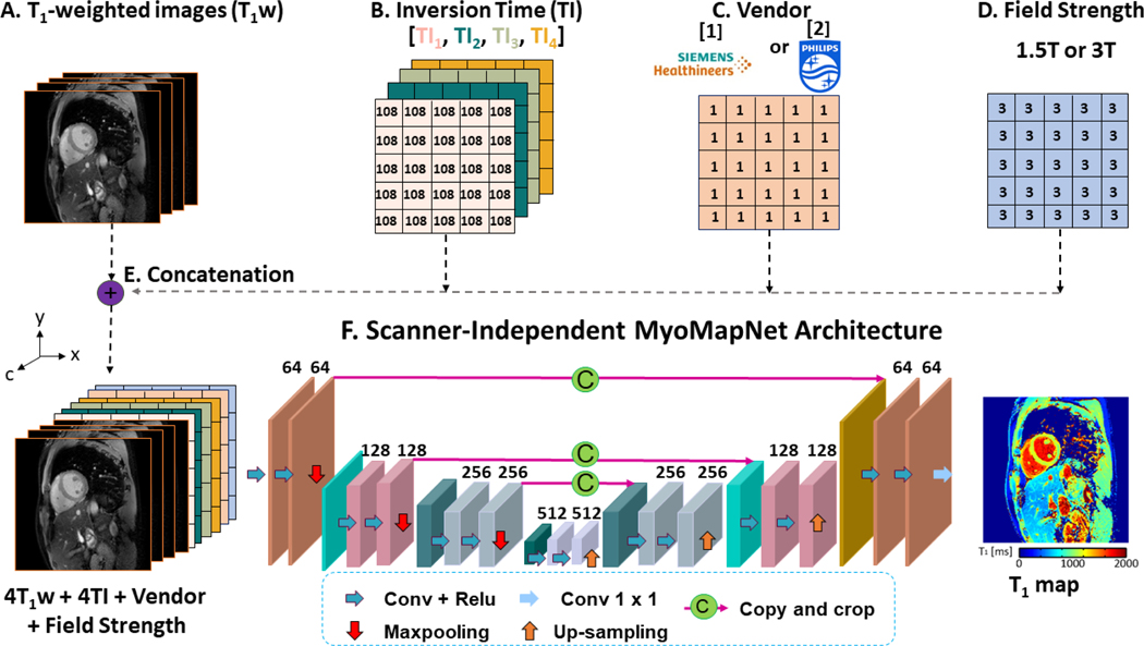
(A) The first four T₁-weighted images extracted from MOLLI are used in SI-MyoMapNet. (B) The corresponding inversion times are encoded into four channels. (C) Vendor is encoded into one channel where 1 for Siemens and 2 for Philips. (D) Field strength is encoded into one channel. (E) The four T₁-weighted images along with the inversion times, vendor and field strength are combined into ten channels, along the c direction and then fed to (F) SI-MyoMapNet, an encoder-decoder neural network to generate a T₁ map.

To incorporate scanner information in the model to make it more generalizable, we modified the MyoMapNet architecture by adding vendor and field strength as additional inputs to the model. The input to SI-MyoMapNet is a ten-channel image where the first four channels consist of the T₁w images, the next four channels comprise the inversion times, and the ninth and tenth channels consist of vendor and field strength respectively (Figure 1A-E). The model is composed of four encoding blocks followed by three decoding blocks. An encoding block is defined as two consecutive convolutional layers followed by a Maxpooling. The number of feature maps for the convolutional layers is 64 in the first encoding block, 128 in the second one, 256 in the third block and 512 in the last. The encoding blocks learn a hierarchical representation of the input data specific to T₁ map generation. These features are translated to the desired output of the network, the T₁ map, through three decoding blocks. The structure of the decoding blocks is similar to that of the encoding blocks, except that Maxpooling is replaced by an up-sampling layer. Up-sampling enables the restoration of spatial dimensions equal to those of the T₁ map. All convolutions are of size 3×3 with a stride of 1×1, a padding of 1×1 and the Maxpooling kernel size is 2×2. To capture nonlinearities between features, a Rectified Linear Unit (ReLU) activation function is applied after each convolution. Skip connections are used to ensure that learning progresses smoothly without vanishing gradient problems (24). The final layer is a convolution with a size of 1×1 and a linear activation function to output the T₁ map (Figure 1F).

Image Acquisition and Analysis

This was a retrospective study with cardiac MR images from three different medical centers. The institutional review boards in the three centers approved the use of cardiac MR data for research with a consent waiver. Patient information was handled in compliance with the Health Insurance Portability and Accountability Act. Cardiac MR images containing myocardial tissue characterization with T₁ mapping images from the three medical centers were included in the study. The three institutions included Beth Israel Deaconess Medical Center (BIDMC), Weill Cornell Medical Center (Cornell) and Boston Medical Center (BMC). All anonymized DICOM images were transferred to BIDMC for development of the model and evaluation. Patients were referred for a clinical cardiac MR scan for different cardiac indications, resulting in a heterogeneous patient cohort, necessary for better evaluation of the model performance. Table 1 summarizes the data characteristics. The images from 1249 (708 male, 56±16 years), 99 (50 male, 52±19 years) and 75 (50 male, 59±14 years), patients from BIDMC, Cornell and BMC respectively were used for training, validation, and testing. The images were collected between 2018 and 2021 using Siemens 3T at BIDMC (MAGNETOM Vida, Siemens Healthineers, Erlangen, Germany), Siemens 1.5T at Cornell (MAGNETOM Sola fit, Siemens Healthineers, Erlangen, Germany), and Philips 1.5T at BMC (Achieva, Philips Healthcare, Best, The Netherlands). MOLLI T₁ mapping was performed at each institution using a vendor-provided imaging protocol. Due to retrospective nature of data collection, different institutions used different vendor imaging protocols. Table 1 provides a detailed description of the imaging protocol from each of the participating medical centers. The native and (or) post-contrast T₁ maps were acquired by vendor provided MOLLI5(3)3 or MOLLI4(1)3(1)2 sequences in BIDMC and Cornell, and by MOLLI5(2)5 or MOLLI5(1)3(1)3 in BMC. Only native T₁ images were available from Cornell. All images were cropped to a matrix size of 160×160 and T₁w intensities were normalized between 0 and 1 prior to processing. Images from BIDMC and Cornell were corrected for motion using vendors-provided inline motion-correction algorithms. Images from BMC were not corrected for motion.

Table 1.

Summary of the datasets from three institutions used in the development of sequence independent MyoMapNet.

	BIDMC		Cornell	BMC
Vendor	Siemens (MAGNETOM Vida)		Siemens (MAGNETOM Sola fit)	Philips (Achieva)
Field Strength	3T		1.5T	1.5T
Sequence	MOLLI5(3)3	MOLLI4(1)3(1)2	MOLLI5(3)3	MOLLI5(2)5	MOLLI5(1)3(1)3
Field of View (mm2)	360×325	360×325	360×325	300×300	300×300
Voxel Size (mm3)	1.7×1.7×8	1.7×1.7×8	1.7×1.7×8	2.2×2.4×10	2.2×2.4×10
Slices	3	3	1	3	3
Flip Angle (º)	35	35	35	35	35
TR (ms)	2.5	2.5	2.82	2.61	2.61
TE (ms)	1.02	1.02	1.08	1.22	1.22
Bandwidth (Hz/Pixel)	1093	1093	1085	1081	1081
Acceleration	GRAPPA R=2	GRAPPA R=2	GRAPPA R=2	SENSE	SENSE
Partial Fourier	7/8	7/8	7/8	6/8	6/8
T1 weighted Images	8	9	8	10	11

Pixel-wise MOLLI T₁ maps were reconstructed offline by fitting T₁w signals ($Si$) at each pixel to a three-parameter model: $Si=A-B\mathrm{*}\mathrm{e}\mathrm{x}\mathrm{p}(-TIi/T_1^{\mathrm{*}})$, where A is the equilibrium magnetization of the tissue, B represents the difference between the magnetization at the first inversion time and the equilibrium magnetization, and T₁* is the apparent T₁ relaxation time. T₁ was calculated as $T_1=\left(\raisebox{1ex}{$B$}\!\left/ \!\raisebox{-1ex}{$A$}\right.-1\right)\mathrm{*}{T}_1^{\mathrm{*}}$. Epicardial and endocardial contours and blood pool (by manually drawing a large region of interest in the blood pool) of the left ventricle were manually delineated by three readers (K.N. with 8 years of experience in cardiac MR contoured 146 cases, E.S. with 9 years of experience contoured 89 cases, and J.C. with 2 years of experience contoured 50 cases). For each subject, T₁ precision was measured by calculating the standard deviation (SD) of pixel-wise T₁ values over myocardium or blood pool. The reported precision is the mean SD over all subjects. The mean and SD of left ventricular myocardial and blood pool T₁ were calculated. The image quality was visually assessed by A.A.

SI-MyoMapNet Training

The training strategy is described in Figure 2. We created the training data by randomly selecting 60% of patients from each of the participating medical centers, with the remaining 40% being equally divided into validation and testing data. The model was trained by minimizing the mean absolute error (MAE) between the reference MOLLI and the estimated T₁ from SI-MyoMapNet from the first four T₁w images extracted from the MOLLI sequence. The model optimization was performed using Adam with an initial learning rate of 0.001, and a weight decay of 0.0001 when the validation loss plateaued, with a mini batch of 64. The MAE for both training and validation was monitored to avoid overfitting and underfitting. The model was implemented using PyTorch version 1.11.0 and trained on an NVIDIA DGX-1 system equipped with 8 Tesla V100 graphics processing units (each with 32 GB memory and 5120 cores) and a central processing unit of 88 cores: Intel Xeon CPU E5–2699 2.20 GHz each, and 512 GB RAM. All codes for training and testing with SI-MyoMapNet model are freely available online (https://github.com/HMS-CardiacMR/Multicenter_MyoMapNet).

Figure 2. Study overview.

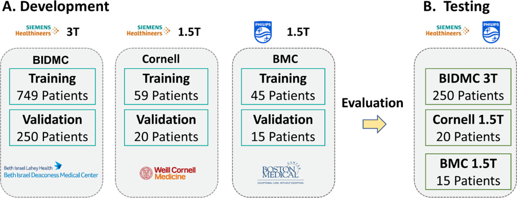
(A) SI-MyoMapNet is trained on a multicenter multivendor dataset with different vendors and field strengths. (B) The model is then tested on a hold-out dataset from the three institutions.

Statistical Analysis

Continuous variables are expressed as mean ± SD. The equivalence test (25) was used to determine whether SI-MyoMapNet and MOLLI were clinically equivalent. The 95% confidence interval (CI) for the mean of the paired differences was calculated, and a margin of equivalence between SI-MyoMapNet and MOLLI of 30 ms was established, based on the reproducibility of the MOLLI sequence (10,11,26). We formulated the null hypothesis that the difference between SI-MyoMapNet and MOLLI is greater than the threshold for equivalence. Errors within the 95% CI were not deemed clinically significant. Linear regression (Pearson correlation coefficient, r) and Bland-Altman analysis were used to investigate the agreement and relationship in T₁ measurements between MOLLI and SI-MyoMapNet. All data analysis was performed using MATLAB R2009b and R2018b (MathWorks, Natick, MA, USA) and Python 3.9.6. Statistical analyses were performed using GraphPad Prism version 9.2.0 (GraphPad Software, San Diego, CA, USA), and Python library scikit-learn (0.19.1).

RESULTS

All T₁ maps were successfully created using SI-MyoMapNet. Figure 3 shows representative native T₁ maps from 3 different subjects, imaged at BIDMC (Siemens 3T), Cornell (Siemens 1.5T) and BMC (Philips 1.5T) from the testing dataset. The SI-MyoMapNet T₁ maps had visually similar image quality as MOLLI sequence.

Figure 3. Native T₁ maps generated using MOLLI and SI-MyoMapNet.

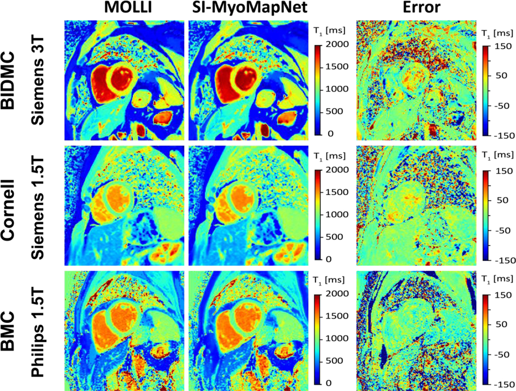
SI-MyoMapNet successfully generated T₁ maps with small errors when compared to MOLLI for data collected using different vendor or field strength.

Figure 4 shows post-contrast maps collected from BIDMC (Siemens 3T) and BMC (Philips 1.5T), demonstrating excellent image quality. Table 2 lists mean and SD values of native and post-contrast T₁ (when available) for the SI-MyoMapNet model and MOLLI measured across BIDMC, Cornell and BMC. Native myocardial and blood T₁ values strongly correlated with MOLLI in BIDMC (Myocardium: r=0.93; Blood: r=0.90), Cornell (Myocardium: r=0.97; Blood: r=0.91), and in BMC (Myocardium: r=0.86; Blood: r=0.90) (Figure 5). SI-MyoMapNet had a mean T₁ difference and SD of 6±1 ms and −10±11 ms in BIDMC, a mean T₁ difference of 6±0 ms and 0±0 ms in Cornell, and a mean T₁ difference of 7±8 ms and 9±11 ms in BMC, for myocardial and blood T₁, respectively.

Figure 4. Post-contrast T₁ maps generated using MOLLI and SI-MyoMapNet across BIDMC and BMC with two different scanners.

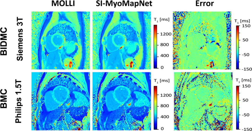
SI-MyoMapNet successfully created excellent T₁ maps compared to MOLLI using only four T₁-weighted images.

Table 2.

Results of SI-MyoMapNet in test data from BIDMC, Cornell and BMC.

	Native T1 (ms)				Post-Contrast T1 (ms)
	Myocardium		Blood		Myocardium		Blood
	T1	Precision	T1	Precision	T1	Precision	T1	Precision
BIDMC 3T Siemens
MyoMapNet	1189±53	68±25	1829±85	32±14	562±64	41±21	441±66	20±18
MOLLI	1183±54	67±23	1839±96	42±25	563±64	39±20	441±67	19±19
Cornell 1.5T Siemens
MyoMapNet	979±46	68±19	1545±94	34±12	N/A	N/A	N/A	N/A
MOLLI	973±46	66±20	1545±94	57±20	N/A	N/A	N/A	N/A
BMC 1.5T Philips
MyoMapNet	1033±54	76±20	1577±93	37±8	497±43	39±12	407±67	46±10
MOLLI	1026±46	77±25	1568±82	45±11	497±43	42±15	411±63	16±9

Figure 5. Linear regression plots for T₁ values estimated with SI-MyoMapNet versus MOLLI for native myocardial and blood T₁ values as calculated for BIDMC, Cornell and BMC.

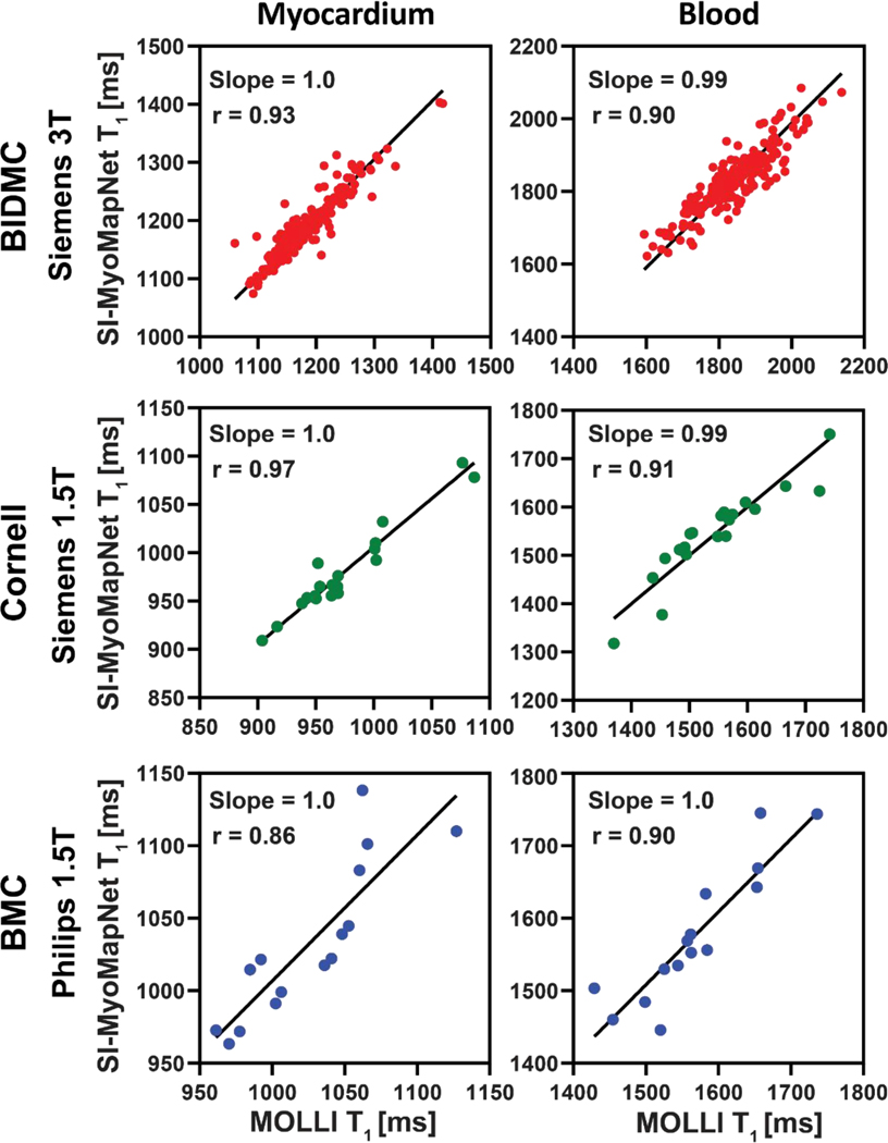
Excellent correlation was observed between SI-MyoMapNet and MOLLI on the three institutions.

In Bland-Altman analysis (Figure 6), good agreement was obtained between SI-MyoMapNet and MOLLI in the three institutions. The 95% CI for Bland-Altman of T₁ differences between SI-MyoMapNet and MOLLI ranged from −34 ms to 44 ms for myocardial T₁ and from −93 ms to 73 ms for blood T₁ in BIDMC, from −17 ms to 28 ms for myocardial T₁ and from −74 ms to 74 ms for blood T₁ in Cornell, and from −45ms to 60 ms for myocardial T₁ and from −70 ms to 86 ms for blood T₁, in BMC.

Figure 6. Bland-Altman plots demonstrating agreement between MOLLI and SI-MyoMapNet for native myocardial and blood T₁ values as calculated for BIDMC, Cornell and BMC.

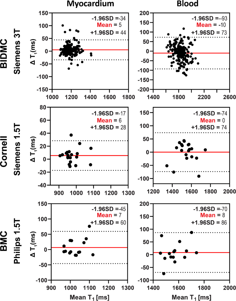
Mean differences and 95% limits of agreement are indicated in red and dotted lines, respectively.

The linear regression (Figure 7) and Bland-Altman (Figure 8) analyses demonstrated SI-MyoMapNet was in excellent agreement with MOLLI for post-contrast T₁ in BIDMC and BMC. Post-contrast myocardial and blood T₁ values strongly correlated with MOLLI in BIDMC (Myocardium: r=0.99; Blood: r=0.99), and in BMC (Myocardium: r=0.95, Blood: r=0.99). The 95% CI for Bland-Altman of T₁ differences between SI-MyoMapNet and MOLLI ranged from −16 ms to 15 ms for myocardial T₁ and from −9 ms to 9 ms for blood T₁ in BIDMC, and from −27 ms to 27 ms for myocardial T₁ and from −19 ms to 10 ms for blood T₁ in BMC.

Figure 7. Linear regression plots for T₁ values estimated with SI-MyoMapNet versus MOLLI for post-contrast myocardial and blood T₁ values as calculated for BIDMC and BMC.

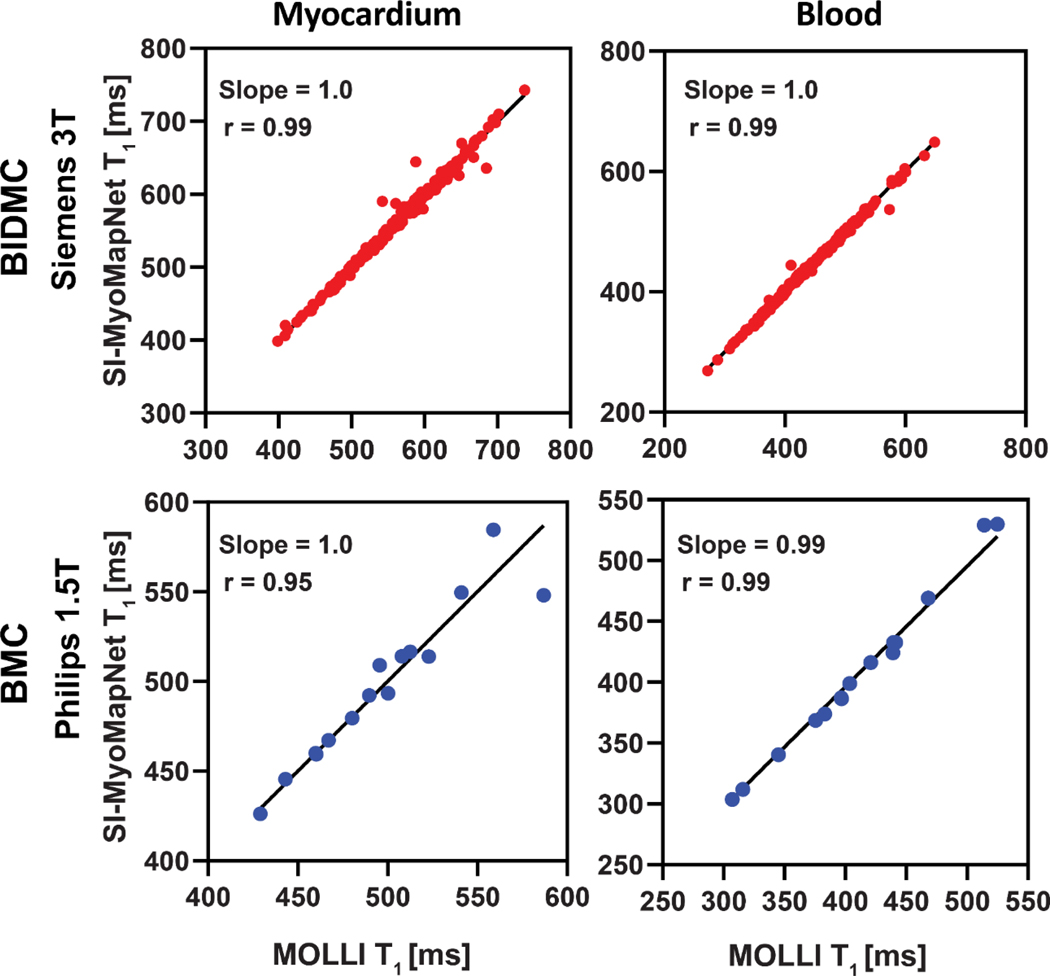
Excellent correlation was observed between SI-MyoMapNet and MOLLI on the two institutions.

Figure 8. Bland-Altman plots demonstrating agreement between MOLLI and SI-MyoMapNet for post-contrast myocardial and blood T₁ values as calculated for BIDMC and BMC.

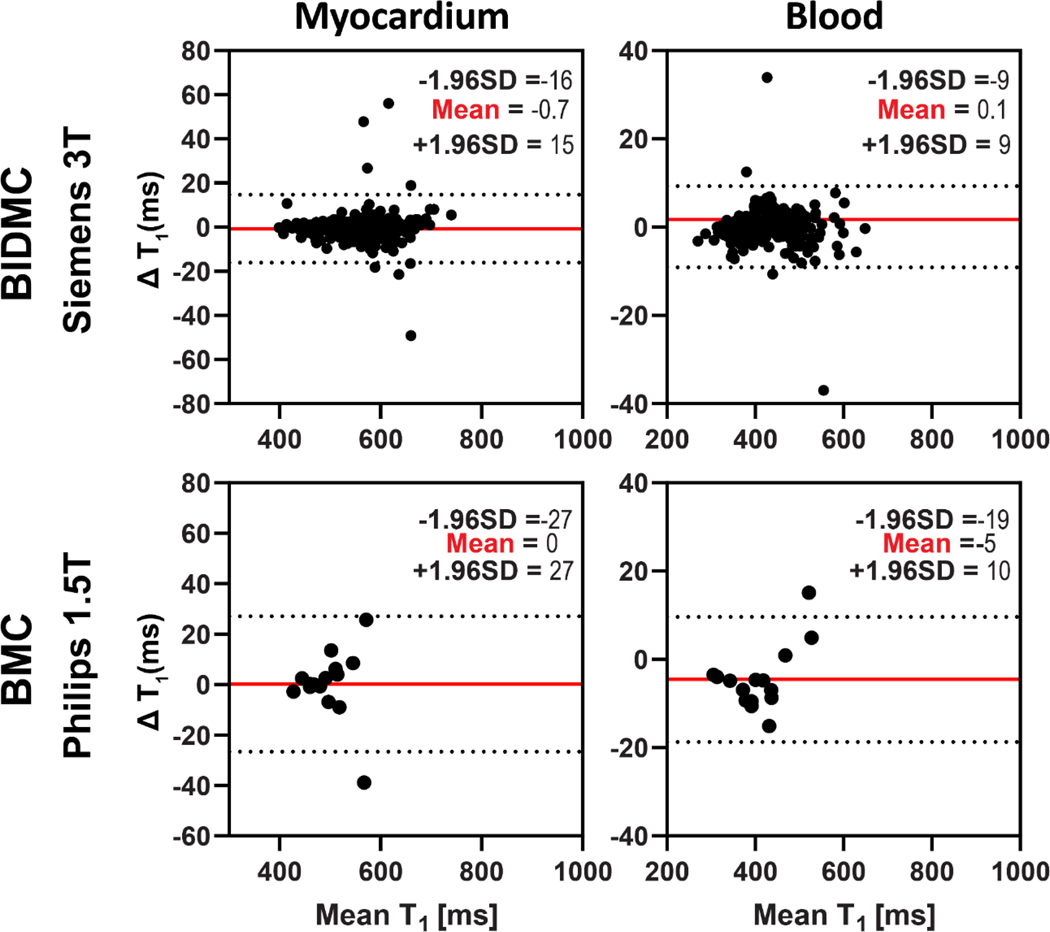
Mean differences and 95% limits of agreement are indicated in red and dotted lines, respectively.

DISCUSSION

In this study, we presented and evaluated an accelerated scanner-independent cardiac T₁ mapping technique that incorporated the scanner information (vendor and field strength) into the T₁ estimation step. The SI-MyoMapNet was successfully trained and tested on data collected using two vendors (Siemens and Philips) and two field strengths (1.5T and 3T). A strong correlation was observed between SI-MyoMapNet and the reference MOLLI across vendors and field strength, demonstrating potential generalizability of the trained model. Although the mean and SD of T₁ values from MOLLI and SI-MyoMapNet were nearly identical for BIDMC: Post contrast T₁, Cornell: native bloodT₁, BMC: post-contrast myocardium T₁, there were still differences in T₁ values between the two techniques, which are not accurately described by the mean and standard deviation of the data (Supplementary Materials).

Standardization in cardiac T₁ mapping remains challenging, and there are known differences in quantitative cardiac T₁ values measured across different vendors (1). Additionally, T₁ values are field strength-dependent. Therefore, a model trained using a single center data may not perform well in other centers, field strengths, or vendors. Various approaches can be used to improve the generalizability of the model, including transfer learning (27,28), using large data representing all scanners, vendors, centers, or domain adaptation (29). By including scanner/vendor information as inputs to the model, the model can learn to account for these differences and adjust its predictions, accordingly, improving its ability to generalize to new datasets. In the proposed architecture, the four T₁w images with their corresponding inversion times were transformed through a series of convolution and max-pooling to a non-linear representation called a latent space. The representation of the data from the three institutions was mixed in the latent space, thus, adding vendors and field strength information could, in theory, help the model to better separate the data from the different systems. Then, the latent space was mapped to the output (T₁ map) that is independent of the scanner by using the decoder.

Statistical methods such as ComBat (30), originally proposed in genomics to adjust for batch effects in gene expression microarray data, have been used to account for the variability in imaging equipment (31,32). Although promising, ComBat has been mainly applied for feature harmonization instead of raw images. De Fauw et. al. (33) used a device adaption branch for optical coherence tomography (OCT) data of the retina to deal with different OCT devices for retina imaging. In SI-MyoMapNet, scanner information was used directly in the model to account for multi-scanner effects. Similarly, an adaption branch could potentially be used in MyoMapNet for data harmonization. Recently, DL-based domain adaptation methods have been proposed as an alternative solution. One of the most important challenges in DL applications is the model generalizability (34). Models may fail when presented with images that were acquired in a different setting or with different parameters from the development dataset (29). Several regularization techniques have been proposed to reduce overfitting and enhance model generalizability, such as reducing model complexity, L1|L2 regularization, dropout or parameter sharing through multi-task learning (35,36). Although these techniques aim to improve generalization, they fail when the external data distribution is different from the development data distribution (37). The basic idea of domain adaptation is to learn a good representation from the training data set (source domain) while approximating the distribution of the test data set (target domain). Further investigation is warranted to study the potential of DL-based domain adaptation in SI-MyoMapNet.

Efficient training of DL-based neural networks requires large datasets. A “sufficient number” of samples is required to ensure the generalizability of the neural network, however estimating the sample size is very challenging (38). In addition to a large sample size, the distribution of the training dataset must represent all data that the model will use in the future. Despite the common belief that additional training samples will yield better model performance, recent studies have reported that large datasets may hurt the model performance (39,40). An alternative solution could be the use of transfer learning, where the model is trained on one dataset, and then fine-tuned on a different smaller dataset to learn the new data distribution. Further studies are needed to evaluate the performance of transfer learning in SI-MyoMapNet.

Limitations

All data were acquired retrospectively for model development and validation. Further studies should be pursued to evaluate the potential of SI-MyoMapNet on a prospectively acquired dataset. Institutes 2 and 3 had smaller databases compared to Institute 1, which implies that Siemens 3T dataset could have influenced the results. Therefore, additional assessments are required to determine the effectiveness of SI-MyoMapNet on alternative datasets. We also only included two vendors, Siemens and Philips and did not have access to suitable data from GE Healthcare. Of further note is that there were differences in the implementation of the MOLLI sequence across different vendors and standardization has been difficult. There are differences in implementation of the MOLLI sequence (e.g., inversion pulse shape, bandwidth, or inversion efficiency), number of phase-encode lines, and image reconstruction techniques. There are also differences in motion correction techniques used for T₁ mapping. These differences could impact blood and myocardium T₁ measurements by different vendors used for training and testing of SI-MyoMapNet. Finally, this study only used data collected using MOLLI and generalizability to other T₁ mapping sequences was not studied. Since, the model was trained using MOLLI data, similar confounders may impact accuracy of the measurements.

Conclusion

In conclusion, the addition of field-strength and vendor as additional information to the deep learning architecture allows generalizability of MyoMapNet, allowing cardiac T₁ mapping using different vendors or field-strength.

References

- 1.Messroghli DR, Moon JC, Ferreira VM, et al. Clinical recommendations for cardiovascular magnetic resonance mapping of T1, T2, T2* and extracellular volume: a consensus statement by the Society for Cardiovascular Magnetic Resonance (SCMR) endorsed by the European Association for Cardiovascular Imaging (EACVI). J Cardiovasc Magn Reson 2017;19(1):1–24. [DOI] [PMC free article] [PubMed] [Google Scholar]
- 2.Puntmann VO, Peker E, Chandrashekhar Y, Nagel E. T1 mapping in characterizing myocardial disease: a comprehensive review. Circ Res 2016;119(2):277–299. [DOI] [PubMed] [Google Scholar]
- 3.Taylor AJ, Salerno M, Dharmakumar R, Jerosch-Herold M. T1 mapping: basic techniques and clinical applications. JACC Cardiovasc Imaging 2016;9(1):67–81. [DOI] [PubMed] [Google Scholar]
- 4.Jellis CL, Kwon DH. Myocardial T1 mapping: modalities and clinical applications. Cardiovasc Diagn Ther 2014;4(2):126. [DOI] [PMC free article] [PubMed] [Google Scholar]
- 5.Chow K, Flewitt JA, Green JD, Pagano JJ, Friedrich MG, Thompson RB. Saturation recovery single-shot acquisition (SASHA) for myocardial T1 mapping. Magn Reson Med 2014;71(6):2082–2095. [DOI] [PubMed] [Google Scholar]
- 6.Xue H, Greiser A, Zuehlsdorff S, et al. Phase-sensitive inversion recovery for myocardial T1 mapping with motion correction and parametric fitting. Magn Reson Med 2013;69(5):1408–1420. [DOI] [PMC free article] [PubMed] [Google Scholar]
- 7.Piechnik SK, Ferreira VM, Dall’Armellina E, et al. Shortened Modified Look-Locker Inversion recovery (ShMOLLI) for clinical myocardial T1-mapping at 1.5 and 3 T within a 9 heartbeat breathhold. J Cardiovasc Magn Reson 2010;12(1):1–11. [DOI] [PMC free article] [PubMed] [Google Scholar]
- 8.Higgins DM, Ridgway JP, Radjenovic A, Sivananthan UM, Smith MA. T1 measurement using a short acquisition period for quantitative cardiac applications. Med Phys 2005;32(6Part1):1738–1746. [DOI] [PubMed] [Google Scholar]
- 9.Weingärtner S, Akçakaya M, Basha T, et al. Combined saturation/inversion recovery sequences for improved evaluation of scar and diffuse fibrosis in patients with arrhythmia or heart rate variability. Magn Reson Med 2014;71(3):1024–1034. [DOI] [PubMed] [Google Scholar]
- 10.Roujol S, Weingärtner S, Foppa M, et al. Accuracy, precision, and reproducibility of four T1 mapping sequences: a head-to-head comparison of MOLLI, ShMOLLI, SASHA, and SAPPHIRE. Radiology 2014;272(3):683–689. [DOI] [PMC free article] [PubMed] [Google Scholar]
- 11.Kellman P, Hansen MS. T1-mapping in the heart: accuracy and precision. J Cardiovasc Magn Reson 2014;16:1–20. [DOI] [PMC free article] [PubMed] [Google Scholar]
- 12.Messroghli DR, Radjenovic A, Kozerke S, Higgins DM, Sivananthan MU, Ridgway JP. Modified Look-Locker inversion recovery (MOLLI) for high-resolution T1 mapping of the heart. Magn Reson Med 2004;52(1):141–146. [DOI] [PubMed] [Google Scholar]
- 13.Kellman P, Wilson JR, Xue H, Ugander M, Arai AE. Extracellular volume fraction mapping in the myocardium, part 1: evaluation of an automated method. J Cardiovasc Magn Reson 2012;14(1):1–11. [DOI] [PMC free article] [PubMed] [Google Scholar]
- 14.Schelbert EB, Testa SM, Meier CG, et al. Myocardial extravascular extracellular volume fraction measurement by gadolinium cardiovascular magnetic resonance in humans: slow infusion versus bolus. J Cardiovasc Magn Reson 2011;13(1):1–14. [DOI] [PMC free article] [PubMed] [Google Scholar]
- 15.Cohen O, Zhu B, Rosen MS. MR fingerprinting deep reconstruction network (DRONE). Magn Reson Med 2018;80(3):885–894. [DOI] [PMC free article] [PubMed] [Google Scholar]
- 16.Zhang Q, Su P, Chen Z, et al. Deep learning–based MR fingerprinting ASL ReconStruction (DeepMARS). Magn Reson Med 2020;84(2):1024–1034. [DOI] [PubMed] [Google Scholar]
- 17.Shao J, Ghodrati V, Nguyen KL, Hu P. Fast and accurate calculation of myocardial T1 and T2 values using deep learning Bloch equation simulations (DeepBLESS). Magn Reson Med 2020;84(5):2831–2845. [DOI] [PMC free article] [PubMed] [Google Scholar]
- 18.Hamilton JI, Currey D, Rajagopalan S, Seiberlich N. Deep learning reconstruction for cardiac magnetic resonance fingerprinting T1 and T2 mapping. Magn Reson Med 2021;85(4):2127–2135. [DOI] [PMC free article] [PubMed] [Google Scholar]
- 19.Guo R, El-Rewaidy H, Assana S, et al. Accelerated cardiac T1 mapping in four heartbeats with inline MyoMapNet: a deep learning-based T1 estimation approach. J Cardiovasc Magn Reson 2022;24(1):1–15. [DOI] [PMC free article] [PubMed] [Google Scholar]
- 20.Amyar A, Guo R, Cai X, et al. Impact of deep learning architectures on accelerated cardiac T1 mapping using MyoMapNet. NMR Biomed 2022:e4794. [DOI] [PMC free article] [PubMed] [Google Scholar]
- 21.Ronneberger O, Fischer P, Brox T. U-net: Convolutional networks for biomedical image segmentation. Int Conf Med Image Comput Assist Interv 2015:234–241. [Google Scholar]
- 22.Le JV, Mendes JK, McKibben N, et al. Accelerated cardiac T1 mapping with recurrent networks and cyclic, model-based loss. Med Phys 2022. [DOI] [PMC free article] [PubMed] [Google Scholar]
- 23.Gottbrecht M, Kramer CM, Salerno M. Native T1 and extracellular volume measurements by cardiac MRI in healthy adults: a meta-analysis. Radiology 2019;290(2):317–326. [DOI] [PMC free article] [PubMed] [Google Scholar]
- 24.Pascanu R, Mikolov T, Bengio Y. On the difficulty of training recurrent neural networks. Proc Mach Learn Int Conf Mach Learn 2013:1310–1318. [Google Scholar]
- 25.Westlake W. Bioequivalence testing--a need to rethink. Biometrics 1981;37(3):589–594. [Google Scholar]
- 26.Shao J, Liu D, Sung K, Nguyen KL, Hu P. Accuracy, precision, and reproducibility of myocardial T1 mapping: A comparison of four T1 estimation algorithms for modified look-locker inversion recovery (MOLLI). Magn Reson Med 2017;78(5):1746–1756. [DOI] [PMC free article] [PubMed] [Google Scholar]
- 27.Torrey L, Shavlik J. Transfer learning. Handbook of research on machine learning applications and trends: algorithms, methods, and techniques: IGI global; 2010. p. 242–264. [Google Scholar]
- 28.Zhu Y, Fahmy AS, Duan C, Nakamori S, Nezafat R. Automated myocardial T2 and extracellular volume quantification in cardiac MRI using transfer learning–based myocardium segmentation. Radiol Artif Intell 2020;2(1). [DOI] [PMC free article] [PubMed] [Google Scholar]
- 29.Wang M, Deng W. Deep visual domain adaptation: A survey. Neurocomputing 2018;312:135–153. [Google Scholar]
- 30.Johnson WE, Li C, Rabinovic A. Adjusting batch effects in microarray expression data using empirical Bayes methods. Biostatistics 2007;8(1):118–127. [DOI] [PubMed] [Google Scholar]
- 31.Fortin J-P, Cullen N, Sheline YI, et al. Harmonization of cortical thickness measurements across scanners and sites. Neuroimage 2018;167:104–120. [DOI] [PMC free article] [PubMed] [Google Scholar]
- 32.Fortin J-P, Parker D, Tunç B, et al. Harmonization of multi-site diffusion tensor imaging data. Neuroimage 2017;161:149–170. [DOI] [PMC free article] [PubMed] [Google Scholar]
- 33.De Fauw J, Ledsam JR, Romera-Paredes B, et al. Clinically applicable deep learning for diagnosis and referral in retinal disease. Nat Med 2018;24(9):1342–1350. [DOI] [PubMed] [Google Scholar]
- 34.Wang F, Casalino LP, Khullar D. Deep learning in medicine—promise, progress, and challenges. JAMA Intern Med 2019;179(3):293–294. [DOI] [PubMed] [Google Scholar]
- 35.Goodfellow I, Bengio Y, Courville A. Deep learning: MIT press: 2016. [Google Scholar]
- 36.Amyar A, Modzelewski R, Vera P, Morard V, Ruan S. Multi-task multi-scale learning for outcome prediction in 3D PET images. Comput Biol Med 2022;151:106208. [DOI] [PubMed] [Google Scholar]
- 37.Zhang C, Bengio S, Hardt M, Recht B, Vinyals O. Understanding deep learning (still) requires rethinking generalization. Commun ACM 2021;64(3):107–115. [Google Scholar]
- 38.Figueroa RL, Zeng-Treitler Q, Kandula S, Ngo LH. Predicting sample size required for classification performance. BMC Medical Inform Decis Mak 2012;12(1):1–10. [DOI] [PMC free article] [PubMed] [Google Scholar]
- 39.Nakkiran P, Kaplun G, Bansal Y, Yang T, Barak B, Sutskever I. Deep double descent: Where bigger models and more data hurt. J Stat Mech Theory Exp 2021;2021(12):124003. [Google Scholar]
- 40.d’Ascoli S, Refinetti M, Biroli G, Krzakala F. Double trouble in double descent: Bias and variance (s) in the lazy regime. Proc Mach Learn Int Conf Mach Learn: PMLR; 2020. p. 2280–2290. [Google Scholar]
Associated Data
This section collects any data citations, data availability statements, or supplementary materials included in this article.