

Abstract
Counting the number of Circulating Tumor Cells (CTCs) for cancer screenings is currently done by cytopathologists with a heavy time and energy cost. AI, especially deep learning, has shown great potential in medical imaging domains. The aim of this paper is to develop a novel hybrid intelligence approach to automatically enumerate CTCs by combining cytopathologist expertise with the efficiency of deep learning convolutional neural networks (CNNs). This hybrid intelligence approach includes three major components: CNN based CTC detection/localization using weak annotations, CNN based CTC segmentation, and a classifier to ultimately determine CTCs. A support vector machine (SVM) was investigated for classification efficiency. The B-scale transform was also introduced to find the maximum sphericality of a given region. The SVM classifier was implemented to use a three-element vector as its input, including the B-scale (size), texture, and area values from the detection and segmentation results. We collected 466 fluoroscopic images for CTC detection/localization, 473 images for CTC segmentation and another 198 images with 323 CTCs as an independent data set for CTC enumeration. Precision and recall for CTC detection are 0.98 and 0.92, which is comparable with the state-of-the-art results that needed much larger and stricter training data sets. The counting error on an independent testing set was 2-3% and 9% (with/without B-scale) and performs much better than previous thresholding approaches with 30% of counting error rates. Recent publications prove facilitation of other types of research in object localization and segmentation are necessary.
Keywords: Circulating tumor cells, enumeration, U-Net, region of interest (ROI), deep learning
I. INTRODUCTION
A. BACKGROUND
Circulating tumor cells (CTCs) originate from the primary tumor mass and travel through the blood to distant bodily locations via circulation [1]. The presence of CTCs in the blood of cancer patients is an important indicator of metastatic disease and resulting treatment speed. The counting of these target cells with highlights based on cellular bodies and structures allows for early cancer detection, prognosis, treatment monitoring, and survival prediction [2], [3]. Liquid biopsy, a method for collection of target cells, allows the analysis of these CTCs, tumor DNA (ctDNA) and exosomes. It is a widely used method in terms of general cancer monitoring [4]. In particular, the identification and characterization of CTCs provides researchers with a goldmine of information that goes beyond just DNA mutations and the cancer itself [5].
B. RELATED LITERATURE
Currently, there are many ways to extract the information embedded inside CTCs. One such way is through manual extraction of information. The CellSearch™ platform is widely used in labs and allows for the detection of CTCs in cancer patients with metastatic breast, prostate or colorectal cancer. However, its emphasis on a single biomarker (an epithelial cell adhesion molecule (EpCAM)-based biomarker) for detection makes it susceptible to false positives and false negatives [6]. Advances in cellular highlighting have made alternatives possible by overlapping the original CellSearch™’s technology with other methods. The CellBrowser software, a handy interface to the CellSearch™ platform, provides an interactive mode to view, count and select cells from the fluorescence images and further output related measurements of the cell [5]. However, the current methods of enumerating CTCs from the fluorescence images, which are manually performed by cytopathologists in the lab, usually take large amounts of effort and is plagued with inefficiency due to potential inexperience and fatigue even in the most experienced of workers [7], [8].
The extensive development in recent years of machine and deep learning automation provides valuable evidence on the effectiveness of automated image analysis. Traditional machine learning techniques have, in the past, been used in cellular enumeration for cancer screening purposes [5], [9], but were usually trained with very limited samples. The classification and detection of CTCs were usually performed after the cells were manually contoured first, and the accuracy of classification was relatively low. Some of the non-traditional-machine-learning techniques include the usage of thresholding as its singular discriminator, providing a simpler method but usually also resulting in a significant error percentage of false positives or false negatives.
While these simple, traditional machine learning and non-machine learning cell enumeration tactics resulted in interesting results, deep learning-based techniques have been successfully used in object detection and segmentation on both natural and medical images. From general topics like general Explainable AI [28], to deep-reinforcement learning [29] and new architectures, like vision transformer (ViT) [27], it is evident many perspectives and tools have been developed for medical image processing.
Several papers have already started to apply deep learning techniques for CTC enumeration [10], [11], [12], [13], [14], [15]. These previous proposals simply applied different convolutional neural networks (CNNs) including VGG16, VGG19 [12], ResNet18, ResNet50 [13], AlexNet [14], [15] and also YOLO-V4 [16] on digital pathology images and reported the CTC counting results. For this type of usage and network designs, there are several flaws. For these approaches [10], [11], [12], [15], the deep learning model needed large amounts of data compared to traditional machine learning models to train. Ranging from between several thousand to tens of thousands of labeled samples, these high quality, manually labeled “ground truth” datasets create significant technical challenges in the training of these models. In addition, some approaches, for example [12], used a strict center-point based method of annotation, while [5] used the CNN for rare CTC detection with a single clear cell image being allowed to be used for training and testing. The YOLO-V4, which was originally designed to recognize cars, humans, trees etc., needed an especially large amount of training samples when it was used for CTC localization during enumeration in [16]. In addition, only one feature - the cell size - was actively considered for detecting/classifying the final CTC labels [16]. A reliance on a single aspect for a multi-featured object declines the performance of any network trained specifically to do such things. In this case, it declines the performance of counting CTCs especially as select CTC cells have a variation on morphology, or when two CTC cells are very close to each other. Important features of the cell such as size or homogeneity that cellular experts and screeners use to enumerate were also not explicitly used in the previous deep learning enumeration models. In other words, it is very hard to correlate the deep learning network results to what information and what features were utilized in beneficially deciding and counting the candidate CTCs. On the other hand, weak annotations from lower time-cost labeling can be more easily acquired in practice but were not suitable for the above, strict, ground truth annotation required deep learning approaches. By modifying methods slightly, weak annotations may be included and a heavy time cost may be saved by their inclusion.
In this paper, rather than strict, tight labels that would surround the CTCs and would force annotators to be extremely diligent to find the centers, the proposed method allows weak annotations of either a rough region of interest (ROI) box or a rough circle near and around the CTC cells (as testing for the effects of labels was also done). For the weak annotated labels in this study, it was not necessary to just have one single CTC cell inside a box, which means non-CTCs can also be included in ROI. Those labels take much less time than those needing careful contouring on each CTC cell [17], being more efficient and more successful in the output/input ratio. We also conceived in this study an approach of using deep learning combined with prior knowledge to enumerate CTCs. Prior knowledge in this experiment includes the encoding of sphericality via the ball-scale transform [18], homogeneity via texture filter, and size estimation. All three features are key points that screeners use, and by integrating them into the network procedure, a hybrid, due to the inclusion of manual features alongside deep learning recognition, and more efficient automated process can be reached.
We have published preliminary results in one conference paper, SPIE [19], but this paper significantly extends the previous version by providing more literatures, different deep learning architectures with more details on methods, and more results from the differing, tested procedures. Through including new, multiple feature-based classifications as compared to before literatures [19], adding the comparation of using circular annotation, and incorporating comparison with existing approaches, this paper aims to conceive a novel and informative comparison of the works in this paper.
The major contribution of this paper is to present a hybrid intelligence (HI) approach for CTC counting by combining cytopathology expertise on CTCs along with the efficiency of machine learning via deep CNNs. Our HI approach includes three main steps: image recognition/detection, segmentation, and classification. The proposed work on weak annotation and B-scale transform technique is more general and can facilitate other types of research in object localization and segmentation.
The paper is arranged as below. Materials and methods are introduced in section II, followed by the qualitative and quantitative results in section III. Section IV discusses and analyzes the results for significance and summarizes the conclusion and limitations as well as the work in the future.
II. MATERIALS AND METHODS
A. OVERVIEW
The methodology of the hybrid intelligence (HI) based automatic CTC enumeration is illustrated in Figure 1. There are three steps in the HI CTC enumeration. Firstly, we localized the regions where possible CTCs are by providing a detected ROI for each one. This requires a CNN for CTC recognition named CNNr. Secondly, we took the resulting ROI as the input for our segmentation network, named CNNs, and further segmented the CTCs within the ROI. Lastly, we enabled a support vector machine (SVM), a previously used classifier in a multitude of medical screenings [32], Cf, for a final determination of the CTC using the ball scale transform with the ROI, as well as the computed features from segmentation.
FIGURE 1.

Methodology of hybrid intelligence system for circulating tumor cell (CTC) enumeration.
B. IMAGE DATA SET AND MATERIALS
This study deals with fluoroscopy images from scanned Circulating Tumor Cells (CTCs). These CTCs were first grown in lab culture and then injected into prepared blood samples. The resulting images were used for deep learning algorithms to test and train them. No patient information was included, as all blood samples had been deidentified prior to the project start. No human subjects were harmed or hurt throughout the duration of this study. The image datasets were summarized in Table 1.
TABLE 1.
Image data allocations.
| Images | CNNr | CNNs | Enumeration |
|---|---|---|---|
| Training | 233 | 236 | one independent testing set 198 images (323 CTCs) |
| Validation | 93 | 95 | |
| Testing | 140 | 142 | |
| Total | 466 | 473 | |
| Size | 1280×1080×3 | 64×64×3 | 1280×1080×3 |
We first gathered viable dataset images for training and testing. In total, we collected 1000+ total CTC positive images for our networks’ (CNNr and CNNs) training and testing phases. 466 total viable images were split in [233:93:140] respectively, for the training, validation, and testing of the detection/localization network; and a total of 473 images were split in [236:95:142] for training, validation, and testing of the segmentation network. Around 1/3 of all images were CTC positive with at least one CTC in the entire image. The ground truths for the detection network in this case were weak box-based annotations for the general cell area. We also investigated another annotation approach using a rough circle to label the CTC in the following sessions.
The support vector machine was trained with a dataset of 66 randomly selected samples from the whole training dataset, split into 30 positive and 36 negative samples. The final CTC enumeration testing datasets are totally independent from any training data set. The enumeration, which is the ultimate goal of this entire endeavor, was tested with another independent testing data set. This includes 198 images with 323 total positive CTCs. There is no overlap between this enumeration testing data set and any other data sets (training and testing) of CNNr or CNNs.
C. METHODS
In this study, CNN based deep learning was utilized to automate the process of CTC enumeration. Instead of only utilizing one network as was done in previous experiments [12], [13], [14], [15], we used two CNNs: CNNr (recognition) and CNNs (segmentation). The aim was to mimic how expert screeners recognize and then double check if CTCs are positive. The two neural networks were used sequentially with the CNNr recognizing the general area where possible CTCs lay first. With those results, it finds those ROIs in the image and then transfers these positive CTC locations to the CNNs. The CNNs only focuses on the highlighted region instead of shifting windows/patches as those in regular segmentation methods [20], [21], [22], providing a more efficient method for cell segmentation. By combining these segmentation results with texture, ball scale value, and cell morphology measurements, these values can be input into the final classification/discrimination of CTCs via SVM.
1). CNNr FOR CTC RECOGNITION/LOCALIZATION
We proposed a center-point based nuclear detection network based on the U-Net framework. The ROI was determined by the location of the center-point as well as the horizontal and vertical distance offsets between the center-point, top-left and bottom-right points as shown in Figure 2.
FIGURE 2.

Box based detection.
The network architecture (using the green channel as an example) of the CNNr is shown in Figure 3. The whole network utilized the UNet network framework as its backbone but with specific parameters changed in accordance for the data in this study. Firstly, the below network (the detection/localization network) resizes the entire fluoroscopy image (1920 × 1080), into smaller, single-CTC positive presence image/patches. Ater training, the CNNr outputs the localization of one CTC via an ROI (region of interest), which gives a preliminary “count” or recognition of CTC cells.
FIGURE 3.
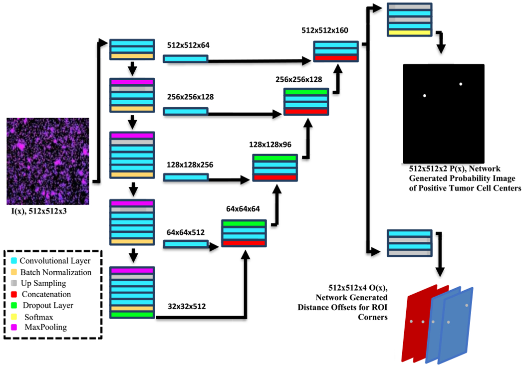
CNNr framework. The outputs include a probability map of the centers, and the 4 distant offset matrixes of corners for the building rectangles.
The specific changes that we made to the U-Net were all for efficiency and compatibility with our purpose. We replaced the de-convolutional layer with an up-sampling layer for reducing the number of parameters. 3 × 3 kernels and 32 output channels (in the middle of U-Net) were used to reduce the redundancy of the feature pyramid. The design of loss function for our network considered both the detection error and the distant offsets with the formular as follows:
| (1) |
where and denote the ground truth of the category and distance offset at pixel represents the possibility value of pixel x classified as ground truth , denotes the predicted distance offset at pixel x, W and Ω represent the parameters of the network and image domains, is the L1-norm, and and serve as trade-off parameters among the three terms. As shown in Figure 3, after training with the given image as an input, we receive the probability map of the centers (which are highlighted, possible regions for two CTC centers - also note that the center of the cell may not be just a single pixel, but rather a center region that consists of a cluster of pixels within a very tight circle, 5×5 in our method.). Then, for each center we have the mapped offsets for indicating the displacement in x and y directions. These correspond to the and in for the predicted corners of the ROI detection box.
We also investigated another network to recognize / localize CTCs by using the weak annotation of center-point based ROI via a rough circle. As seen in Figure 4, the center point at from the rough circle (in white) is not the real CTC center, which is shown as the red dot. Due to that weakness/non-strictness of our annotations, we first refined the location ground truth before using it in our deep learning networks as seen below. We extracted the coordinate information of a labeled region’s center, and then built one circle with a radius of 5 pixels around that center point. The background and pixels in the center-point circles were annotated with labels “0” and “1”. We then utilized the refined annotation data to train the CNNs network for segmenting the center-point circles from fluorescence images (by using one output channel representing the probability map of segmentation which will derived the center point at ), and also predicting the distance offset between any surrounding pixels and the center-point (by using two output channels representing probability maps of distance offset in the x and y directions separately) as shown in Figure 5. The loss function for our network also considered classes and distance offsets, which is the same as equation 1.
FIGURE 4.

Weak annotation using center-point based ROI via a circle.
FIGURE 5.

The center point-based detection method using rough cycle labels during training is seen above, with two distance offset and a center-based probability map of the centers.
After training, for each pixel in the testing image, we were able to check every pixel’s maximum possible circular region and the displacements (distance offset in x and y). The final calculated center point . So, in Figure 5, we can find that the output of the distance offset is different now with only two distance offsets - red for 1 distance delta x and blue for delta y.
2). CNNs FOR CTC SEGMENTATION
The secondary segmentation network, CNNs, follows a similar architecture to that of the above CNNr but uses the cropped tumor cell masks as training samples instead. The segmentation network will “cut-out”/overlay a mask delineating the circulating tumor cell’s boundaries. The result can be utilized for feature extraction such as to provide prior information of size, homogeneity, and texture of CTCs, a vital contribution that this work aimed to improve. By taking the localized regions from the detection network, the segmentation network is more efficient by checking only at those regions with high probabilities in terms of positive presence of CTC centers.
DICE, a statistic that is commonly chosen for segmentation network reporting, has a large bias towards object size [22]. Due to the small cell size of CTCs, we instead designed the loss function of this segmentation network directly using the FP (false positive) & FN (false negative) as below,
| (2) |
where is the ground truth at pixel x and are the segmentation results at x.
3). BALL SCALE
The B-scale transform was originally developed and utilized for object segmentations in MRI and CT images [11], [12]. We are the first to adopt it into digital pathology according to our knowledge. Given an image where C is the 2D/3D (which can be nD) array of pixels, and f is an intensity function defined on C, for each pixel , the B-scale image has the pixel value of the maximum radius for a circle, which covers a region with the sufficient homogeneous with c. The maximum radius is achieved by continuously comparing a fraction with a given threshold (ts = 0.85),
| (3) |
where is the number of pixels in (i.e., volume of) and is the homogeneity function using a zero-mean unnormalized Gaussian function. More details about can be found in [18].
4). CLASSIFIER FOR FINAL DETERMINING CTCs
CTC recognition roughly finds and estimates the number of CTCs. We can thus further refine and confirm the final CTC number by utilizing classifiers. We applied the traditional sophisticated classifier, Support Vector Machine (SVM), using three features as the inputs.
The pixel value in a B-scale image is the maximum ball radius for that pixel (according to the homogeneity defined inside the ball [18]). B-scale provides the information that allows us to enhance the image by encoding the object size (ball radius) and the object shape (how similar it is to a ball) information. These B-scaled images can also be used as an additional input channel for UNet, and can also be used for refining the output from deep learning for CTC enumeration. This additional knowledge of maximum radius size is a great beneficiary for efficiency and results and can be used as one feature for SVM. We also considered the area of segmentation results as the 2nd feature. The third important feature is the texture information. Texture as a feature was calculated by using co-occurrence-based approach with entropy as target function, and with parameter of win size, [23]. Encoded with a texture filter, we can input the resulting value into the SVM. The transparent input of each feature in the Support Vector Machine achieves the initial target of making a hybrid, easily analyzable network for determining beneficial and harmful features to recognition.
5). DATA AUGMENTATION AND PLATFORM SETTING
To increase the number and diversity of training data, we varied the intensity level of the image by multiplying the pixel-wise intensity value with scale factors 0.9 and 1.1. All experiments were conducted on a PC with an Intel i7-7700K CPU and two NVIDIA 1080 Ti GPUs with RAM of 11Gbytes. Unfortunately, due to the image size of detection dataset being too large, the storage capacity of the GPU was not enough to construct the detection network. All deep learning network used the Stochastic gradient descent (SGD) optimizer. Therefore, we resized the input image with scale factors 0.5 for the detection network and, in total, it took us 8 hours for 500 epochs of training for the detection network. It cost around 1 hour to train the segmentation network (using ROI region as the input) and using specific cropped samples for 1000 epochs training.
III. RESULTS
A. QUALITATIVE RESULTS
1). WEAK ANNOTATIONS FOR CTC LOCALIZATION
Figure 6 shows the weak annotations in their respective differences: box-labels and circle-labels. Compared to stricter and higher-quality annotations which require an exact contour or tight bounding box around the CTC, these labels took much less energy and time. In this method, the CTCs and their neighboring regions are included in the labeled region, which can provide more information and facilitate the training for achieving a more effective localization model. In other words, the presence of CTCs in those regions were found to be successful in rough counts, showing our CNNr training on weak-annotation data provides good effort/output ratio. Figure 7. shows the original image and the B-scale image after the transform was completed. With heightened contrast between the brightened CTC cell area and darkened background, the images strongly suggests B-scale enhances the CTCs for further detection and enumeration. These B-Scale images allow us to find the largest circle/sphericity in a given area in 2D/3D space with adequate homogeneity, and each pixel in B-scale image gets a radius value. The successful highlights from our experiment evidence that the ball scale transform can be used as a tool for pre-processing on the image and as a tool for providing useful features for further classifiers as shown in the following sections. Figure 8 shows different CTC detection/recognition results via box for some difficult cases. Figure 9 shows the segmentation results compared with the ground truth (GT) of a manual segmentation of a CTC.
FIGURE 6.

Illustration of weak annotations on CTCs: original image (l), rough circle (middle) and box (r).
FIGURE 7.

Illustration of the B-scale transform on digital pathology images.
FIGURE 8.

Different CTC detection/recognition results via box for some difficult cases.
FIGURE 9.

Illustrations of the original image with the manual segmentation (GT) and automatic segmentation (Auto-seg) of two example CTCs samples.
2). EVALUATION MATRIX
Precision (TP / (TP + FP)) and Recall (TP / (TP + FN)) were two common factors used for evaluating detection results. The CTC counting error, Ec, is equal to |Ng-Nc|/Ng, with Ng as the real number of the CTCs as the ground truth value, and Nc is the number of CTC from the enumeration approaches.
3). ESTIMATION OF THE NON-CTC CELLS
To provide a more detailed and accurate diagnostic of our results, we had to determine the total number of non-CTCs. In this study, an averaging statistical method was used to estimate all the non-CTCs in any image (1920 × 1080). This worked by setting an image-center based rectangular sample region with the size of 192 × 108, and then counting the number of cells within this sampling region. By dividing the number of cells with the scale factor of the sampling (1% of total image dimensions), the total amount of estimated cells in the entire image is calculated. This estimation process was performed on 20 randomly selected training images. The total number of cells can be estimated by checking the ratio of the area of the whole image (excluding the exposed region in the images, such as the left top corner in Figure 8) to the area of sampling region. The amount of total non-CTCs can then be obtained by subtracting the number of CTCs in the current image from the total estimated cells for the whole image. Through such computation, we calculated there to be around 400,000 non-CTCs in the testing images.
4). ESTIMATION OF CTC DETECTION, SEGMENTATION AND ENUMERATION
Table 2 summarized the results from the proposed approach using box labels for CTC ground truth location. In this study, we proposed approaches to enumerate CTCs via detecting and segmenting CTCs, and then using an SVM for the final CTC determination. We evaluated our detection network (CNNr) using Precision and Recall, and evaluated our segmentation network (CNNs) using DICE. These results were reported in Table 2, despite segmentation itself not being the purpose of this study. It is important to note that the segmentation for CTCs was only performed for the deep learning approach using box labels in this study. In addition, through segmentation results, we obtained our morphologic information of the cell which is inputted into the SVM. For the purpose of comparison, we also listed the results by using a separate thresholding action on the green channel, which seems to be an intrinsic and straight approach.
TABLE 2.
CTC recognition, segmentation and enumberation performance on testing set.
| Methods | Recognition | Segmentation | Enumeration | |
|---|---|---|---|---|
| Precision | Recall | DICE | CTC counting error, Ec | |
| SVM | 0.98, 0.10 | 0.92, 0.18 | 0.85, 0.08 | without B-scale 0.09 |
| SVM with B-scale 0.03 | ||||
| Threshold (Baseline) | 0.82, 0.15 | 0.96, 0.13 | 0.69, 0.14 | 0.30 |
Note: Ec=|Ng-Nc|/Ng, with Ng as the real number of the CTCs as the ground truth value, and Nc is the number of CTC from the automatic enumeration approaches.
The lowest CTC counting error, Ec, on the independent data set was 0.03 through using the deep learning with box labels following CNNr+CNNs+SVM in this study. Without using the B-scale filter, Ec was 0.09, which was still much better than that from commonly done threshold approaches (0.30) that are prevalent in the field now. Meanwhile, our method is comparable with the results in even the most recent publication [11], which reported sensitivity and specificity as 0.95 and 0.92 but required a significantly larger training data set. More details of the comparisons among different approaches can be found in Table 3. Compared with other related methods, our method applied a simple CNN architecture. Our testing datasets were relatively equal to some [5], [24], or were dwarfed by those in [11], [16], and [26]. Even with our weak annotations, our performance is comparable and outperform most algorithms using strict and high quality labels in training. In addition, our usage of CTC positives is noteworthy. Reference [11] only used 139 CTCs in testing, and the resulting performance on its training dataset was much lower than that in testing set. This generally indicates that the CNN was not well trained, meaning more samples were needed, as ours provided. Reference [26], in addition, only used very limited CTCs, with only 31 total in testing. Reference [24] had lower sensitivity and specificity of 90.3 and 91.3% with no previous knowledge (cell size, etc. that our paper provided) being adopted. Reference [30] used a larger training dataset (5699 images) and very strict annotation for ground truth with two experts manually bounding boxes around CTCs and cross-checking the results. Yet, our method is still very comparable with its results.
TABLE 3.
CTC enumeration approach comparisons.
| Literatures | Approach overview | Data allocations | CTC annotation methods | Performance | |
|---|---|---|---|---|---|
| G. Da Col, et al. [5] | Using traditional machine learning with man-crafted image features | A total of 2,598 cells from 45 MBC patients with 846 CD45 pos cells and 344 eCTC in training. | interactive mode to select interested cells and calculated features | 91% accuracy with eCTC | 84% with CD45pos |
| Z. Guo, et al. [11] | Automatic enumeration of CTCs with pure deep learning (RESNET18) and transfer learning assistance | 694 CTC images (5% of all cells) including 555 for training and 139 for testing; 13472 non-CTC (95%) was down sampled to 555 | contouring each CTC are needed for training; non-CTC are also needed to be segmented for training purpose | 95.3% (sensitivity) 91.7% (specificity) | counting error: 5.4% (training) vs. 3.6% (testing) |
| S. Wang, et al. [16] | Apply YOLO-V4 on CTC counting | 8 advanced-stage cancer patient samples; 6 normal samples | manual tight bounding box for each cell for training | an average precision (AP) of 98.63%, 99.04%, and 98.95% for cancer cell lines HT29, A549, and KYSE30. | |
| M. Yu, et al. [24] | Segmentation results of all nucleis (CTCs and non-CTCs) from edge detection were used by a CNN for CTC detection | 2300 cells from 600 patients with 1300 cells for training, 1000 cells fro testing (700 non-CTC cells and 300 CTC cells); | The Manual Interpretation of CTCs Counting is needed. CTCs and non-CTCs manual segmentation are needed. | The sensitivity and specificity of 90.3 and 91.3%. | No previous knowledge was adopted. |
| MG Krebs et al. [25] | Use the man-crafted features in classification. | 699 cells in total, 80% for training. Not clear the number of CTCs vs. non-CTCs. | Manual labeling on the CTC types. | SVM with 10 features achieved the AUC of 0.99. | |
| Satelli, et al. [26] | Crop CTC and non-CTC images are used for training a CNN to determinating CTCs | A total number of 120 cells (31 cultured cells and 89 WBCs) were tested. | Manually crop images of both CTC and non-CTC for training | No report on CTC counting errors. | It cannot handle two cells who are close to each other. |
| Shen, et al. [30] | Using computer vision preprocessing and ensemble generic deep learning with pretrained model from COCO data | mCTC with total 7623 images (5699 training and 1924 testing); CAF with total 702 images (455 training and 247 testing) | Two experts to do bounding box around CTCs manually, with the 2nd expert refining the labels from the 1st expert (high time cost of annotations) | Precision 94% recall 96% for mCTC | Precision 93% recall 84% for CAF |
| HI Method (This Paper) | Hybrid intelligence: using auto-segmented results and features with SVM for discriminating CTCs. | 1070 CTCs for deep learning model training with another 323 CTCs for enumeration | Drawing a “weak” Box or rough circle around CTCs | Box Detection with Precision 0.98, Recall 0.92 | SVM Enumeration with counting error 0.03. |
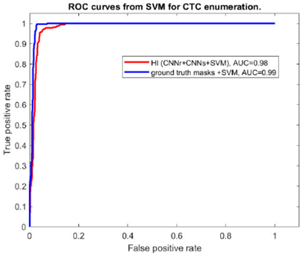
Figure 10. shows the ROC curve of the final CTC determination from SVM using the features of size, B-scale value and texture. Red ROC curve is for the results from the proposed approach following CNNr+CNNs+SVM. The AUC is close to 1 which means the enumeration achieved good performance after SVM classification.
FIGURE 10.
ROC curves of CTC enumeration from SVM.
The blue curve is used for the purpose of comparing SVM using the features from the automatic via CNNr+CNNs vs. the feature from the ground truth masks. These two ROCs are very close to each other, which means the automatic localization and segmentation have the similar performance as the idea scenario. In the above experiments, 860 random selected non-CTCs were used together with 323 CTCs in SVM classifier for achieving the ROC. Although it is not the purpose of this paper to test different classifiers, we evaluated the random forest classifier with AUC 0.82 and accurate 0.84. We had a simliar conclusion comparing SVM with the random forest method as in [31]. It seems that SVM performs better in general than random classifiers on the limited training dataset.
5). FURTHER EXPLORATION ON BOX LABELS VS. CIRCLE BASED LABELS
Figure 11 shows the challenge of CTC detection using models being trained with labels via rough circle annotation (left and middle) or box annotation (right). The CNNr, using the rough circle-based labels, can localize the two neighboring CTCs. However, it missed a cell (labelled via white arrows). In most cases, the CNNr using the box-based annotation seems to have caught more CTCs and performed better (illustrated in Table 4). The detection approach using box labels achieved better detection and enumeration results (0.03 vs. 0.08 of counting error), which indicates that the box from manual labeling involved more interesting information from neighboring regions than just the circle labels on the CTC cell itself. The inclusion of the image background, in other words, could be of vital importance for the neural networks for detection to work efficiently.
FIGURE 11.

Illustration of CTC detection results from the proposed CNN by using circle-based labels (left and middle) and box-based labels (right) during training.
TABLE 4.
CTC detection and enumeration on the testing set using CNN being trained via circle labels vs. box labels.
| Methods | Detection | Segmentation | Enumeration | |
|---|---|---|---|---|
| Precision | Recall | DICE | Counting error, Ec | |
| Detect CTC using circle labels | 0.80 | 0.88 | - | 0.08 |
| Detect CTC using box labels | 0.98 | 0.92 | 0.85 | 0.03 |
IV. CONCLUSION
In this paper, we proposed a novel hybrid intelligence approach for CTC enumeration, which includes CTC automatic recognition/ detection, CTC automatic segmentation and three vector, and SVM based classification to enumerate CTCs. The CNN for the CTC detection network was trained using weak annotations with rough circles and boxes labeling the CTC locations. B-scale transform was introduced to enhance digital pathology images and provide the SVM discriminator with homogeneity, size, and spherical shape of the CTC for estimation information. Our method is comparable and competitive with the results in recent publications. We also investigated CTC detection by using different labels: circle label ground truth location vs. box labeling ground truth location, which is very interesting and has not been reported before. The proposed approach and framework are flexible and can be easily propagated to other types of research of locations and detection. The number of samples in this study is limited since it is only from one center. The limited number of samples could be a constraint on deep learning training and affect deep learning performance. We are trying to collect more samples for both training and testing in the ongoing work. In addition, our paper’s focus was on developing a structured method to automatically enumerate CTCs. With its current success, we are now not limited by the structure and can explore ablational experiments to narrow further which variables benefited our method. It also interests us to check different deep learning architectures, such as the recent machine learning vision transformer [27], reinforcement learning strategies [33] and different training methodologies on this task in the future.
ACKNOWLEDGMENT
We acknowledge the open-source software of CAVASS from Medical Image Processing Group at the University of Pennsylvania, which were used for obtaining our texture and ball scale transform values.
This work was supported by the National Cancer Institute under Grant R37CA255948 and Grant R01CA230339.
Biographies

LEIHUI TONG is currently pursuing the Diploma degree with the Conestoga Senior High School, PA, USA, and the Diploma (Medical Experience Associate) degree with the Chester County Intermediate Unit, PA, USA.
In 2020, he was a first Research Volunteer and then a Student Internship Scholar working on medical image analysis with the Medical Image Processing Group, University of Pennsylvania. He is also a Research Volunteer on the Circulating Tumor Cell Enumeration Project with The Pq Laboratory of BiomeDx/Rx, Department of Biomedical Engineering, Binghamton University. His research interests include the intersection between medicine, science, and AI.
Mr. Tong holds a student membership of SPIE—Medical Imaging (the International Society for Optics and Photonics) and a membership of the International MENSA of the Largest and Oldest High-IQ Society. He is also recognized nationally as a National Merit Scholar and a National Merit Finalist Candidate.

YUAN WAN received the M.D. degree in clinical medicine and the M.S. degree in genetics from Southeast University, Nanjing, China, in 2004 and 2007, respectively, and the Ph.D. degree in bioengineering from The University of Texas at Arlington, Arlington, TX, USA, in 2012.
In 2007, he was with Shanghai Biochip Corporation as the Vice Director of Research and Development. From 2012 to 2015, he was a Research Associate with the University of South Australia, Adelaide, Australia. Later, he joined the MINIBio Laboratory, The Penn State University, and took his postdoctoral training, from 2015 to 2018. From 2018 to 2023, he was an Assistant Professor in biomedical engineering with Binghamton University. He was promoted to an Associate Professor, in 2023. He is the author of more than 70 articles and three patents. His research interests include translational medicine, including cancer liquid biopsy, artificial intelligence-based cancer diagnosis, drug delivery systems, bioinformatics, and relevant clinical implementations.
Dr. Wan was a recipient of the National Cancer Institute R01 Subaward, in 2018, R37 MERIT Award, in 2021, and the Early State Distinguished Research Award from Binghamton University, in 2022.
Footnotes
This work involved human subjects or animals in its research. Approval of all ethical and experimental procedures and protocols was granted by the Office of Research Compliance, Binghamton University under Application No. 020BIO00000041.
REFERENCES
- [1].Hao S-J, Wan Y, Xia Y-Q, Zou X, and Zheng S-Y, “Size-based separation methods of circulating tumor cells,” Adv. Drug Del. Rev, vol. 125, pp. 3–20, Feb. 2018. [DOI] [PubMed] [Google Scholar]
- [2].Rack B, Schindlbeck C, Jückstock J, Andergassen U, Hepp P, Zwingers T, Friedl TWP, Lorenz R, Tesch H, Fasching PA, Fehm T, Schneeweiss A, Lichtenegger W, Beckmann MW, Friese K, Pantel K, and Janni W, “Circulating tumor cells predict survival in early average-to-high risk breast cancer patients,” JNCI: J. Nat. Cancer Inst, vol. 106, no. 5, May 2014, Art. no. dju066. [Online]. Available: https://academic.oup.com/jnci/article/106/5/dju066/2607122?login=true [DOI] [PMC free article] [PubMed] [Google Scholar]
- [3].Poveda A, Kaye SB, McCormack R, Wang S, Parekh T, Ricci D, Lebedinsky CA, Tercero JC, Zintl P, and Monk BJ, “Circulating tumor cells predict progression free survival and overall survival in patients with relapsed/recurrent advanced ovarian cancer,” Gynecologic Oncol., vol. 122, no. 3, pp. 567–572, Sep. 2011. [DOI] [PubMed] [Google Scholar]
- [4].Alix-Panabières C and Pantel K, “Clinical applications of circulating tumor cells and circulating tumor DNA as liquid biopsy,” Cancer Discovery, vol. 6, no. 5, pp. 479–491, May 2016. [DOI] [PubMed] [Google Scholar]
- [5].Da Col G, Del Ben F, Bulfoni M, Turetta M, Gerratana L, Bertozzi S, Beltrami AP, and Cesselli D, “Image analysis of circulating tumor cells and leukocytes predicts survival and metastatic pattern in breast cancer patients,” Frontiers Oncol., vol. 12, Feb. 2022, Art. no. 725318. [Online]. Available: 10.3389/fonc.2022.725318/full [DOI] [PMC free article] [PubMed] [Google Scholar]
- [6].Wang L, Balasubramanian P, Chen AP, Kummar S, Evrard YA, and Kinders RJ, “Promise and limits of the cellsearch platform for evaluating pharmacodynamics in circulating tumor cells,” Seminars Oncol., vol. 43, no. 4, pp. 464–475, Aug. 2016. [DOI] [PMC free article] [PubMed] [Google Scholar]
- [7].Aceto N, Bardia A, Miyamoto DT, Donaldson MC, Wittner BS, Spencer JA, Yu M, Pely A, Engstrom A, Zhu H, Brannigan BW, Kapur R, Stott SL, Shioda T, Ramaswamy S, Ting DT, Lin CP, Toner M, Haber DA, and Maheswaran S, “Circulating tumor cell clusters are oligoclonal precursors of breast cancer metastasis,” Cell, vol. 158, no. 5, pp. 1110–1122, Aug. 2014. [DOI] [PMC free article] [PubMed] [Google Scholar]
- [8].Yang Y-P, Giret TM, and Cote RJ, “Circulating tumor cells from enumeration to analysis: Current challenges and future opportunities,” Cancers, vol. 13, no. 11, p. 2723, May 2021. [DOI] [PMC free article] [PubMed] [Google Scholar]
- [9].Hatzidaki E, Iliopoulos A, and Papasotiriou I, “A novel method for colorectal cancer screening based on circulating tumor cells and machine learning,” Entropy, vol. 23, no. 10, p. 1248, Sep. 2021. [DOI] [PMC free article] [PubMed] [Google Scholar]
- [10].Wang S, Yao J, Petrick N, and Summers RM, “Combining statistical and geometric features for colonic polyp detection in CTC based on multiple kernel learning,” Int. J. Comput. Intell. Appl, vol. 9, no. 1, pp. 1–15, Mar. 2010. [DOI] [PMC free article] [PubMed] [Google Scholar]
- [11].Guo Z, Lin X, Hui Y, Wang J, Zhang Q, and Kong F, “Circulating tumor cell identification based on deep learning,” Frontiers Oncol., vol. 12, Feb. 2022, Art. no. 843879. [Online]. Available: 10.3389/fonc.2022.843879/full [DOI] [PMC free article] [PubMed] [Google Scholar]
- [12].Liu Q, Junker A, Murakami K, and Hu P, “Automated counting of cancer cells by ensembling deep features,” Cells, vol. 8, no. 9, p. 1019, Sep. 2019. [DOI] [PMC free article] [PubMed] [Google Scholar]
- [13].Simonyan K and Zisserman A, “A very deep convolutional networks for large-scale image recognition,” 2014, arXiv:1409.1556. [Google Scholar]
- [14].Russakovsky O, Deng J, Su H, Krause J, Satheesh S, Ma S, Huang Z, Karpathy A, Khosla A, Bernstein M, Berg AC, and Fei-Fei L, “ImageNet large scale visual recognition challenge,” Int. J. Comput. Vis, vol. 115, no. 3, pp. 211–252, Dec. 2015. [Google Scholar]
- [15].Krizhevsky A, Sutskever I, and Hinton GE, “ImageNet classification with deep convolutional neural networks,” Commun. ACM, vol. 60, no. 6, pp. 84–90, May 2017, doi: 10.1145/3065386. [DOI] [Google Scholar]
- [16].Wang S, Zhou Y, Qin X, Nair S, Huang X, and Liu Y, “Label-free detection of rare circulating tumor cells by image analysis and machine learning,” Sci. Rep, vol. 10, p. 12226, Jul. 2020. [DOI] [PMC free article] [PubMed] [Google Scholar]
- [17].Stevens M, Nanou A, Terstappen LWMM, Driemel C, Stoecklein NH, and Coumans FAW, “StarDist image segmentation improves circulating tumor cell detection,” Cancers, vol. 14, no. 12, p. 2916, Jun. 2022. [DOI] [PMC free article] [PubMed] [Google Scholar]
- [18].Baǧci U, Udupa JK, and Chen X, “Ball-scale based hierarchical multi-object recognition in 3D medical images,” Proc. SPIE, vol. 7623, Mar. 2010, Art. no. 762345. [Google Scholar]
- [19].Tong L and Wan Y, “Deep learning combined with ball scale transform for circulating tumor cell enumeration in digital pathology,” Proc. SPIE, vol. 12471, Apr. 2023, Art. no. 1247111. [Google Scholar]
- [20].Su H, Xing F, Kong X, Xie Y, Zhang S, and Yang L, “Robust cell detection and segmentation in histopathological images using sparse reconstruction and stacked denoising autoencoders,” Med. Image Comput. Comput. Assist. Intervent, vol. 9351, pp. 383–390, Nov. 2015. [DOI] [PMC free article] [PubMed] [Google Scholar]
- [21].Al-Kofahi Y, Zaltsman A, Graves R, Marshall W, and Rusu M, “A deep learning-based algorithm for 2-D cell segmentation in micro scopy images,” BMC Bioinf., vol. 19, no. 1, Dec. 2018, Art. no. 365. [Online]. Available: 10.1186/s12859-018-2375-z#citeas [DOI] [PMC free article] [PubMed] [Google Scholar]
- [22].Mechrez R, Goldberger J, and Greenspan H, “Patch-based segmentation with spatial consistency: Application to MS lesions in brain MRI,” Int. J. Biomed. Imag, vol. 2016, 2016, Art. no. 7952541. [Online]. Available: https://www.hindawi.com/journals/ijbi/2016/7952541/ [DOI] [PMC free article] [PubMed] [Google Scholar]
- [23].Eelbode T, Bertels J, Berman M, Vandermeulen D, Maes F, Bisschops R, and Blaschko MB, “Optimization for medical image segmentation: Theory and practice when evaluating with dice score or Jaccard index,” IEEE Trans. Med. Imag, vol. 39, no. 11, pp. 3679–3690, Nov. 2020. [DOI] [PubMed] [Google Scholar]
- [24].Reifegerste S, Hampel U, and Poll R, “Texture-based image segmentation in medical volume images,” Biomed Tech, vol. 47, pp. 9–786, Jan. 2002. [Online]. Available: 10.1515/bmte.2002.47.s1b.786/html [DOI] [PubMed] [Google Scholar]
- [25].Yu M, Stott S, Toner M, Maheswaran S, and Haber DA, “Circulating tumor cells: Approaches to isolation and characterization,” J. Cell Biol, vol. 192, no. 3, pp. 373–382, Feb. 2011. [DOI] [PMC free article] [PubMed] [Google Scholar]
- [26].Krebs MG, Hou J-M, Sloane R, Lancashire L, Priest L, Nonaka D, Ward TH, Backen A, Clack G, Hughes A, Ranson M, Blackhall FH, and Dive C, “Analysis of circulating tumor cells in patients with non-small cell lung cancer using epithelial marker-dependent and -Independent approaches,” J. Thoracic Oncol, vol. 7, no. 2, pp. 306–315, Feb. 2012. [DOI] [PubMed] [Google Scholar]
- [27].Satelli A, Brownlee Z, Mitra A, Meng QH, and Li S, “Circulating tumor cell enumeration with a combination of epithelial cell adhesion molecule–and cell-surface vimentin–based methods for monitoring breast cancer therapeutic response,” Clin. Chem, vol. 61, pp. 66–259, Jan. 2015. [DOI] [PMC free article] [PubMed] [Google Scholar]
- [28].Dosovitskiy A, Beyer L, Kolesnikov A, Weissenborn D, and Zhai X, Unterthiner T, Dehghani M, Minderer M, Heigold G, Gelly S, Uszkoreit J, Houlsby N, “An image is worth 16 × 16 words: Transformers for image recognition at scale,” 2021, arXiv:2010.11929. [Google Scholar]
- [29].Vilone G and Longo L, “Notions of explainability and evaluation approaches for explainable artificial intelligence,” Inf. Fusion, vol. 76, pp. 89–106, Dec. 2021, doi: 10.1016/j.inffus.2021.05.009. [DOI] [Google Scholar]
- [30].Najar A and Chetouani M, “Reinforcement learning with human advice: A survey,” Frontiers Robot. AI, vol. 8, Jun. 2021, Art. no. 584075. [DOI] [PMC free article] [PubMed] [Google Scholar]
- [31].Shen C, Rawal S, Brown R, Zhou H, Agarwal A, Watson MA, Cote RJ, and Yang C, “Automatic detection of circulating tumor cells and cancer associated fibroblasts using deep learning,” Sci. Rep, vol. 13, no. 1, p. 5708, Apr. 2023. [DOI] [PMC free article] [PubMed] [Google Scholar]
- [32].Murugan A, Nair SAH, and Kumar KPS, “Detection of skin cancer using SVM, random forest and kNN classifiers,” J. Med. Syst, vol. 43, no. 8, p. 269, Aug. 2019. [DOI] [PubMed] [Google Scholar]
- [33].Krishnan MMR, Banerjee S, Chakraborty C, Chakraborty C, and Ray AK, “Statistical analysis of mammographic features and its classification using support vector machine,” Expert Syst. Appl, vol. 37, no. 1, pp. 470–478, Jan. 2010. [Google Scholar]
- [34].Lakhan A, Mohammed MA, Obaid OI, Chakraborty C, Abdulkareem KH, and Kadry S, “Efficient deep-reinforcement learning aware resource allocation in SDN-enabled fog paradigm,” Automated Softw. Eng, vol. 29, no. 1, p. 20, May 2022. [Google Scholar]