Improving Reliability of Magnetic Localization Using Input Space Transformation

Abstract

Body motion tracking for medical applications has the potential to improve quality of life for people with physical or speech motor disorders. Current solutions available in the market are either inaccurate, not affordable, or are impractical for a medical setting or at home. Magnetic localization can address these issues thanks to its high accuracy, simplicity of use, wearability, and use of inexpensive sensors such as magnetometers. However, sources of unreliability affect magnetometers to such an extent that the localization model trained in a controlled environment might exhibit poor tracking accuracy when deployed to end users. Traditional magnetic calibration methods, such as ellipsoid fit (EF), do not sufficiently attenuate the effect of these sources of unreliability to reach a positional accuracy that is both consistent and satisfactory for our target applications. To improve reliability, we developed a calibration method called post-deployment input space transformation (PDIST) that reduces the distribution shift in the magnetic measurements between model training and deployment. In this paper, we focused on change in magnetization or magnetometer as sources of unreliability. Our results show that PDIST performs better than EF in decreasing positional errors by a factor of ~3 when magnetization is distorted, and up to ~7 when our localization model is tested on a different magnetometer than the one it was trained with. Furthermore, PDIST is shown to perform reliably by providing consistent results across all our data collection that tested various combinations of the sources of unreliability.

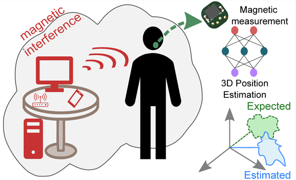
Graphical Abstract

I. Introduction

AS wearable devices have become more capable, people are more willing to have sensors attached to their body. This is a boon for the field of body motion tracking by opening new opportunities in applications such as interactive graphics, virtual and augmented reality, motion capture, computer-aided surgery, and rehabilitation [1], [2]. Although optical tracking is commonly used due to its high accuracy [1]–[4], it cannot be used outside of few applications (e.g., research on human motion, entertainment industry) because it requires purchasing an expensive camera setup and controlling lighting conditions to work effectively.

Therefore, there is a need for an alternative solution that would be affordable and practical to be used in any environment. Inertial measurement units (IMUs) are becoming ubiquitous sensors for tracking due to their low cost, small size, and their robustness to various environmental conditions. However, inertial sensing based on IMUs cannot track position as accurately as optical methods because of parasitic motion artifacts and positional drift due to the integration of sensor noise over time [1], [5]. To overcome these issues, hybrid tracking systems combining inertial sensing with other motion capture methods have been developed to improve overall tracking performance [2], [5]. In our previous work [6], [7], we developed a hybrid method that combined magnetic tracking and inertial sensing by using a 9D IMU (accelerometer, gyroscope, and magnetometer) as a tracer. The 2D orientation of the tracer (roll and pitch) is estimated from the inertial data provided by the accelerometer and gyroscope, and its 3D position is estimated from the magnetic measurements of the magnetometer. The details of our orientation-compensated magnetic localization can be found in [6]. In sum, a local magnetic field is created for a target volume by permanent magnets placed at fixed locations in a wearable attachment. As the IMU tracer moves within this volume, its estimated orientation is used to rotate its magnetic measurements into a reference frame, and the resulting data are fed into a neural network that generates 3D positional estimates.

Neural networks are shown to be successful function approximators for magnetic localization providing low positional errors in the range of few millimeters for a tongue tracking application. They generalize well when trained and tested on the same magnetometer, in the same session, and in the same magnetic environment [6], [8]. However, the reported tracking performance might drastically decrease in practice because of at least two problems. First, a magnetometer's magnetization can be affected when brought too close to a ferrous object during shipping, storage, or even in use. Sources of change in magnetization are ubiquitous, from the frame of a table to the electric cables in the wall, or even from electronic devices and monitors. Change in magnetization poses a challenge to the reliability of a localization model since the same magnetometer would then output a different magnetic measurement for the same position. Depending on the level of change in magnetization, the differences in magnetic measurements can be significant, and thus this change cannot simply be considered as noise during localization model training. Moreover, the effect of change in magnetization is random and thus cannot be accounted for in the localization model.

Secondly, creating a localization model for each magnetometer is not scalable because it requires a significant amount of time to collect individual training and validation datasets. Therefore, the localization model must be transferable across magnetometers which is another challenge because magnetometers are slightly different due to process variations during manufacturing. This results in small differences in magnetic measurements by any two magnetometers at the same position, resulting in errors large enough to prevent the system from being used in applications requiring sub-millimeter accuracy (e.g., tongue tracking [6]).

For high-precision magnetic localization using feed-forward neural networks, these two problems (Fig. 1), i.e., change in magnetization/magnetometer, cannot be solved by the commonly used calibration method that relies on finding a better approximation of the underlying true magnetic field such as ellipsoid fit [9]–[11] or more complex methods that align magnetometer axes with a gyroscope or accelerometer [12]–[15]. A successful calibration strategy should aim at obtaining magnetic field measurements from the same input space that was used during training of the localization model to reduce the localization errors due to the change of magnetization/magnetometer.

Fig. 1.

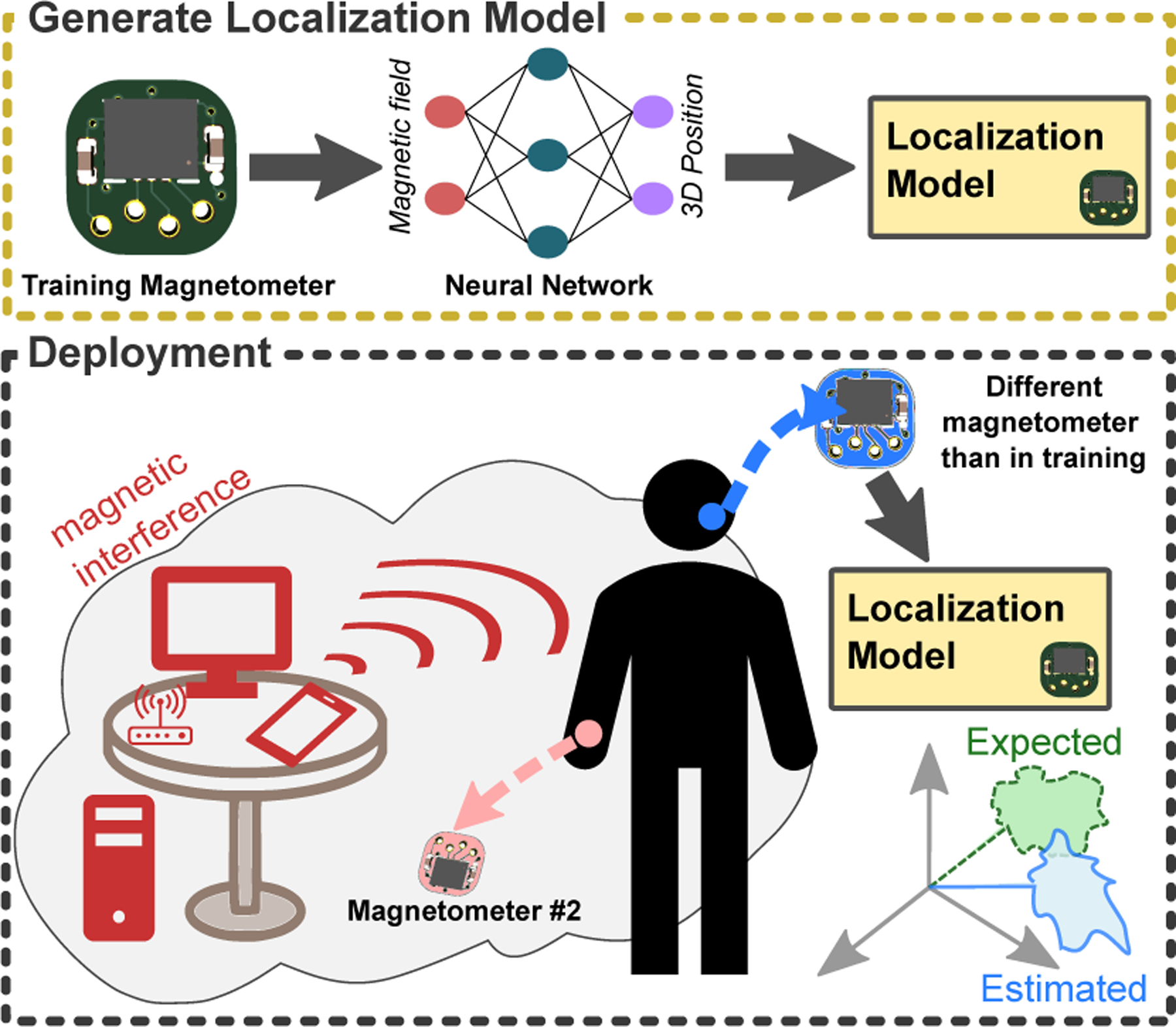
Overview of the problem of reliability with magnetic localization in which the change in magnetization and the use of a trained model on different magnetometers cause unreliable localization post-deployment.

In summary, there is a reliability issue in magnetic localization that is caused by a distribution shift [16], [17] of magnetic measurements (input) that changes its relationship to the magnetometer's positions (output) due to disturbances that are both intrinsic (differences between magnetometers) and extrinsic (change in magnetization). In this paper, our main contributions can be summarized as follows:

1. We developed a novel method, called post-deployment input space transformation (PDIST), that reduces distribution shift to improve reliability.

2. We collected multiple datasets with different magnetization/magnetometer configurations and provided detailed analysis on the effectiveness of the PDIST.

The rest of the paper is organized as follows: Section II provides a mathematical description of the reliability issues along with a description of our PDIST method, Section III describes our data collection, Section IV presents our results on tracking accuracy and a discussion on the effectiveness of the PDIST, and Section V concludes on the significance and impact of this work.

II. Magnetic Localization

A. Mathematical Background

The objective of magnetic localization is to estimate the 3D position of a magnetometer, $\mathbf{y}\in {ℝ}^3$, from its magnetic measurement, $\mathbf{x}\in {ℝ}^3$, that is moving inside a target volume ${𝒱}_p$. The output space $𝓞$ is composed of all possible positions of the magnetometer in the target volume and the input space $𝓘$ comprises of all possible magnetic measurements. The localization model is the mapping function $f$ between the input and output spaces such that

$$\begin{array}{c}𝓞=\left\{{\mathbf{y}}_i\mid {\mathbf{y}}_i\in {𝒱}_p,{\mathbf{y}}_i\in {ℝ}^3\right\},\\ 𝓘=\left\{{\mathbf{x}}_i\mid {\mathbf{x}}_i=f^{-1}\left({\mathbf{y}}_i\right),{\mathbf{y}}_i\in {𝒱}_p,{\mathbf{x}}_i\in {ℝ}^3\right\}.\end{array}$$

The output space $𝓞$ is usually defined first to meet the tracking requirement for a target application. Then, the input space $𝓘$ is determined by the strength and placement of the magnets. Therefore, the aim of magnetic localization is to find $\widehat{f}:𝓘\to 𝓞$, an approximation of $f$, so that given a magnetic measurement $\mathbf{x}$, the position of the magnetometer, can be estimated by $\widehat{\mathbf{y}}=\widehat{f}\left(\mathbf{x}\right),\widehat{\mathbf{y}}\in {ℝ}^3$, where $\widehat{f}$ is optimized to minimize the 2-norm of the localization error, i.e., $\parallel \mathbf{y}-\widehat{\mathbf{y}}{\parallel }_2$.

B. Sources of Unreliability

When deploying a magnetic localization model, there are two main sources of unreliability that can significantly worsen tracking accuracy. The first source is change in magnetization due to hard-iron and soft-iron disturbances. We define the current magnetization of a magnetometer as a magnetic frame of reference (FoR) representing 3D magnetic readings that can be perturbed by magnetic disturbances. Hard-iron disturbances resulting from permanent magnetizations by nearby magnetic objects are reflected on FoR as an offset, whereas, soft-iron disturbances caused by nearby materials with high magnetic permeability result in more complex alterations in FoR, both of which lead to changes in the magnetization of the magnetometer [15], [18]. The second source of unreliability comes from variations during the manufacturing of magnetometers [19], [20]. This results in different magnetometers having slightly different coordinate frames of measurement, due to, for example, axial misalignment and non-uniform axial gains.

Regardless of the source of unreliability, the problem remains the same: a magnetometer post-deployment will measure magnetic fields differently than expected. More specifically, let $\mathbf{x}$ and $\tilde{\mathbf{x}}$ denote a magnetic measurement recorded during training and after the localization model is deployed, respectively. The magnetic measurements obtained at a fixed position $\mathbf{y}$ in ${𝒱}_p$, denoted by ${\left.\mathbf{x}\right|}_{\mathbf{y}}$ and ${\left.\tilde{\mathbf{x}}\right|}_{\mathbf{y}}$, will be different because of the source(s) of unreliability, i.e., ${\left.\mathbf{x}\right|}_y\ne {\left.\tilde{\mathbf{x}}\right|}_y$. Hence, the localization model that was trained using ${\left\{\left({\left.{\mathbf{x}}_i\right|}_{{\mathbf{y}}_i},{\mathbf{y}}_i\right)\right\}}_{i=1}^N$, where $N$ stands for the number of samples, will provide a worse tracking accuracy, i.e., $\parallel \widehat{f}\left({\left.\tilde{\mathbf{x}}\right|}_{\mathbf{y}}\right)-\mathbf{y}{\parallel }_2>>\parallel \widehat{f}\left({\left.\mathbf{x}\right|}_{\mathbf{y}}\right)-\mathbf{y}{\parallel }_2$.

C. Issues with Traditional Magnetic Calibration

To increase reliability, the standard procedure is to calibrate each magnetometer using a linear model as follows,

$${\mathbf{x}}^c=\mathbf{A}\mathbf{x}+\mathbf{b}$$ (1)

where ${\mathbf{x}}^c\in {ℝ}^3$ represents the magnetic measurement of a calibrated magnetometer, $\mathbf{A}$ is a compact matrix that corrects for soft-iron magnetic disturbances, non-orthogonality of axes, and sensitivity, while $\mathbf{b}$ represents hard-iron disturbance.

Ellipsoid fit (EF) is the most common calibration method that calculates $\mathbf{A}$ and $\mathbf{b}$ in (1) by relying on the constant norm of the Earth's magnetic field [9]–[11]. The magnetometer is rotated along all three dimensions of rotation, usually randomly and by hand. The resulting magnetic measurements form a 3D ellipsoid, and the objective of EF is to find $\mathbf{A}$ and $\mathbf{b}$ that transform the measurements into a sphere. However, EF does not explicitly return the orientation of the sphere [12], [13] which results in obtaining different FoRs after changes in magnetization/magnetometer. Though EF calibration is likely sufficient for most magnetic sensing applications, variations in FoR are preventing our localization from consistently reaching sub-millimeter positional accuracy for our tracking applications.

To obtain a reproducible FoR across sessions, alternative methods of calibration relying on axis alignment with gyroscopes and accelerometers were designed [12]–[15]. These methods require the calibration of a gyroscope and accelerometer in addition to the magnetometer, and have infeasible assumptions for our system. Furthermore, any additional error made during the calibration of these devices at the time of deployment by an end user of our application, such as unwanted linear acceleration, might result in considerable localization errors. More importantly, these methods do not directly address the problem of preserving the FoR that was used during model training, and fail to return consistent measurements. Instead of aligning the magnetometer's FoR with those of other sensors, a better method might be to align the FoR observed post-deployment with the one from training, which is the purpose of our proposed post-deployment input space transformation (PDIST).

D. Post-Deployment Input Space Transformation

For the rest of the paper, we define the training dataset of magnetic measurements as $D_T={\left\{\left({\mathbf{x}}_i,{\mathbf{y}}_i\right)\right\}}_{i=1}^N$, and a deployment dataset as $\tilde{D}={\left\{\left({\tilde{\mathbf{x}}}_i,{\tilde{\mathbf{y}}}_i\right)\right\}}_{i=1}^{\tilde{N}}$, where $N$ and $\tilde{N}$ are the number of samples. $\tilde{D}$ is collected post-deployment by the user and for an actual tracking session.

For the localization model to generalize well to the deployment set, the joint probability distribution $p\left(\mathbf{x},\mathbf{y}\right)$ should be the same across training and deployment. This implies that the function $\widehat{f}:{ℝ}^3\to {ℝ}^3$ obtained by training the model on $D_T$ should provide sufficient information to generalize to $\tilde{D}$. One natural assumption is that if the magnetic measurements are recorded at the same locations, i.e. ${\mathbf{y}}_i={\tilde{\mathbf{y}}}_i$, it should hold that $\widehat{f}\left({\mathbf{x}}_i\right)=\widehat{f}\left({\tilde{\mathbf{x}}}_i\right)$, $\forall i\in \left\{1,\dots ,N\right\}$ and $N=\tilde{N}$. However, we found that even though $p\left(\mathbf{y}\right)=p\left(\tilde{\mathbf{y}}\right)$ since the data is collected on the same set of locations, we observe that $p\left(\mathbf{x}\mid \mathbf{y}\right)\ne p\left(\tilde{\mathbf{x}}\mid \tilde{\mathbf{y}}\right)$, and this implies $p\left(\mathbf{x},\mathbf{y}\right)\ne p\left(\tilde{\mathbf{x}},\tilde{\mathbf{y}}\right)$. The difference between these distributions explain the degradation in the model's performance after deployment.

To enable the localization model $\widehat{f}$ trained on $D_T$ to make accurate predictions on $\tilde{D}$, our PDIST method was designed to project the deployment input space $\widetilde{𝓘}$ back into the training input space ${𝓘}_T$ by using a mapping function $\mathbf{G}:\widetilde{𝓘}\to {𝓘}_T$ that is found by following this procedure:

1. Collect a one-time sampling of ${𝓘}_T$ before training, and denote as $D_T^Q={\left\{\left({\mathbf{x}}_i^Q,{\mathbf{y}}_i^Q\right)\right\}}_{i=1}^{N^Q}$.

2. Collect a sampling of $𝓘$ before every new tracking session (post-deployment), and denote as ${\tilde{D}}^Q={\left\{\left({\tilde{\mathbf{x}}}_i^Q,{\mathbf{y}}_i^Q\right)\right\}}_{i=1}^{N^Q}$.

3. Find the best $\mathbf{G}$ that minimizes ${\sum }_{i=1}^{N^Q}‖{\tilde{\mathbf{x}}}_i^Q-{\mathbf{x}}_i^Q‖$.

The number of samples $N^Q$ is the same for both datasets and should be low enough to reduce the duration of this calibration since it must be performed by end users before each tracking session. In this paper, we found empirically that 24 is a suitable number of samples since collecting more samples increases the effort but does not increase the performance substantially. These samples are collected from the same predefined set of positions ${\mathbf{y}}_i^Q$ that is carefully selected to be equally distributed throughout the volume ${𝒱}_p$ to improve the quality of the mapping $\mathbf{G}$. Although experimental evidence suggests that the mapping between the input spaces might be non-linear, we found that a linear transformation captures most of the variation, which also enables the use of linear regression as a fast and reliable optimization method.

More formally, let ${\mathbf{X}}_T^Q\in {ℝ}^{N^Q\times 3}$ and ${\tilde{\mathbf{X}}}^Q\in {ℝ}^{N^Q\times 3}$ represent the magnetic measurements collected at ${\mathbf{Y}}^Q\in {ℝ}^{N^Q\times 3}$ for the training and deployment sets. Let $\mathbf{Z}=\left[\begin{array}{ll}1\hfill & {\tilde{\mathbf{X}}}^Q\hfill \end{array}\right]$, $\mathbf{Z}\in {ℝ}^{N^Q\times 4}$, where the column vector $\mathbf{1}$ is added to incorporate the offset term. The transformation $\mathbf{G}\in {ℝ}^{4\times 3}$ can be estimated using linear regression as follows,

$$\mathbf{G}={\left({\mathbf{Z}}^T\mathbf{Z}\right)}^{-1}{\mathbf{Z}}^T{\mathbf{X}}_T^Q$$ (2)

$\mathbf{G}$ can be further decomposed as $\mathbf{G}=\left[\begin{array}{c}{\mathbf{g}}_o^T\\ {\mathbf{G}}_R\end{array}\right]$, where ${\mathbf{g}}_{\mathbf{o}}^{\mathbf{T}}\in {ℝ}^3$ is the offset, while ${\mathbf{G}}_{\mathbf{R}}\in {ℝ}^{3\times 3}$ consists of scaling, rotation and cross-gain terms. Setting $\tilde{\mathbf{Z}}=\left[\begin{array}{ll}\mathbf{1}\hfill & \tilde{\mathbf{X}}\hfill \end{array}\right]$, the PDIST-calibrated magnetic measurements of the deployment set $\tilde{\mathbf{X}}\in {ℝ}^{\tilde{N}\times 3}$ is then,

$$\widehat{\mathbf{X}}=\tilde{\mathbf{Z}}\mathbf{G}.$$ (3)

To demonstrate how PDIST is connected to EF, let ${\mathbf{x}}^{true}$ and $\mathbf{x}$ denote the true Earth magnetic field reading and the measured magnetic field, respectively. EF implicitly tries to find a relation between true and measured magnetic fields through $\mathbf{A}$ and $\mathbf{b}$ when applied to both the training and deployment sets, where

$${\mathbf{x}}_T={\mathbf{A}}_1{\mathbf{x}}^{true}+{\mathbf{b}}_1$$ (4)

$$\tilde{\mathbf{x}}={\mathbf{A}}_2{\mathbf{x}}^{true}+{\mathbf{b}}_2$$ (5)

for the training and deployment sets, respectively.

Instead, PDIST solves for the deployment set

$${\widehat{\mathbf{x}}}_T={\mathbf{G}}_R\tilde{\mathbf{x}}+{\mathbf{g}}_o.$$ (6)

which removes the need to calculate ${\mathbf{A}}_1$, ${\mathbf{A}}_2$, ${\mathbf{b}}_1$, ${\mathbf{b}}_2$ in relation to true magnetic field readings. Instead, PDIST directly relates ${\widehat{\mathbf{x}}}_T$ and ${\mathbf{x}}_T$ by minimizing their difference ${‖{\widehat{\mathbf{x}}}_T-{\mathbf{x}}_T‖}_2$. Thus, using (4) and (5), and assuming perfect transformation, i.e., ${\mathbf{x}}_T={\widehat{\mathbf{x}}}_T$, (6) can be written as

$${\mathbf{A}}_1{\mathbf{x}}^{true}+{\mathbf{b}}_1={\mathbf{G}}_R\left({\mathbf{A}}_2{\mathbf{x}}^{true}+{\mathbf{b}}_2\right)+{\mathbf{g}}_o$$ (7)

$$={\mathbf{G}}_R{\mathbf{A}}_2{\mathbf{x}}^{true}+{\mathbf{G}}_R{\mathbf{b}}_2+{\mathbf{g}}_o$$ (8)

Consequently, we find that ${\mathbf{G}}_R={\mathbf{A}}_1{\mathbf{A}}_2^{-1}$ and ${\mathbf{g}}_o={\mathbf{b}}_1-{\mathbf{G}}_R{\mathbf{b}}_2$. Poor reliability can be explained by the fact that ${\mathbf{A}}_1$ and ${\mathbf{A}}_2$ are not necessarily equal, as well as ${\mathbf{b}}_1$ and ${\mathbf{b}}_2$ although ${\mathbf{x}}^{true}$ remains the same. The reason is that magnetic measurements denoted by ${\mathbf{x}}_T$ and $\tilde{\mathbf{x}}$ are not in the same FoR anymore due to aforementioned factors. Across sessions, EF is not capable of finding a consistent transformation, encoded by ${\mathbf{A}}_1$, ${\mathbf{A}}_2$ and ${\mathbf{b}}_1$, ${\mathbf{b}}_2$, required for positional accuracy because its underlying optimization problem does not take into account the orientation of its FoR. In other words, the measurement sets used for calculating ${\mathbf{A}}_1$, ${\mathbf{b}}_1$ and ${\mathbf{A}}_2$, ${\mathbf{b}}_2$ pairs are independent from each other and do not calibrate the magnetic readings to exactly the same FoR. On the contrary, PDIST is effective because it uses a fixed set of measurements ${\mathbf{x}}_T$ and $\tilde{\mathbf{x}}$ to explicitly transform FoR of the latter into the former's. This helps to estimate the drift in the FoR reducing the difference between training and deployment input spaces. Fig. 2 illustrates the difference between EF and PDIST and their effect on localization accuracy.

Fig. 2.

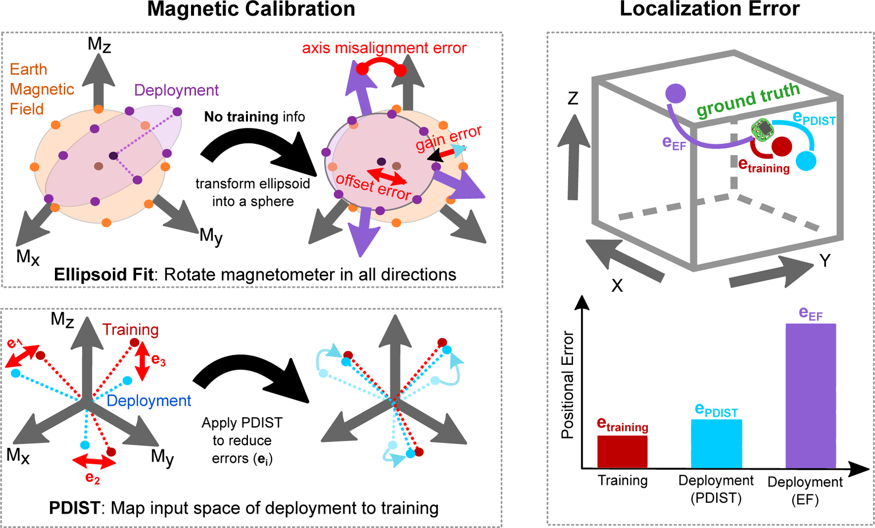
Illustration of the difference in localization accuracy (right) when calibrating a magnetometer with EF (top left) and PDIST (bottom left).

III. Data Collection

A magnetic localization model is first trained on a magnetometer, and then tested in two separate experiments that simulated a post-deployment environment by (1) changing the magnetization of the training magnetometer and (2) replacing it with another magnetometer. The data collection was performed with EF and PDIST to evaluate the effect of calibration on reliability. Since this work is part of a research project whose aim is to develop an articulograph for tongue tracking, ${𝒱}_p$ is selected to encompass the volume of the oral cavity.

A. Experiment Setup

Fig. 3 shows the 5D positioning stage that was used to accurately place the magnetometer in any desired 3D position. Although our positioning stage can also control the orientation of the magnetometer, this paper focuses only on investigating reliability for 3D positioning since the impact of rotation on tracking accuracy and reliability is a completely separate problem that will be studied in future work. However, we would refer interested readers to the previous work in [6] for an analysis of performance of the localization model with orientation. The 9D IMU used in this study is a BMX160 (Bosch Sensortec, Reutlingen, Germany) that includes an accelerometer, gyroscope and magnetometer. As shown in Fig. 3, up to three IMUs can be used simultaneously to collect multiple datasets at a sampling frequency of 125 Hz. The local magnetic field is produced by an array of magnets embedded inside an eyewear that was designed for a wearable tongue tracking application. Rotary motor encoders provide the ground-truth 3D position of the IMU, and the center of the nose bridge area on the eyewear is selected as the origin. The unit of magnetic measurements is Least Significant Bit (LSB) for which 1 LSB is equal to 3 milligauss, and output positions are in millimeters (mm).

Fig. 3.

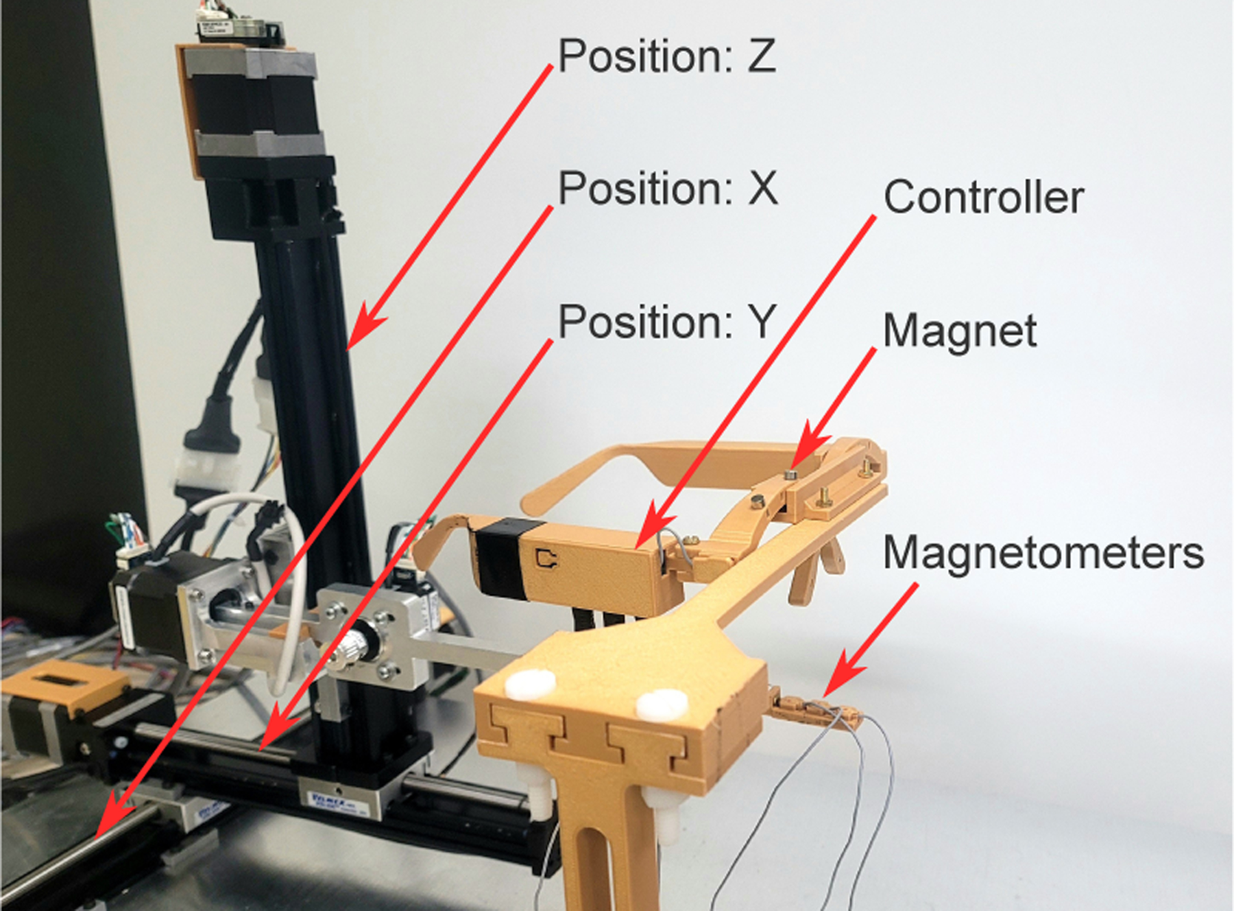
Experiment setup in which a local magnetic field is generated by permanent magnets embedded in an eyewear.

B. Localization Model Training

Fig. 4 shows the training, validation and testing trajectories that are sampled within a volume of $10\times 12\times 9{\text{cm}}^3$. They are collected sequentially to reduce the possibility of a change in magnetization during this session. The number of magnetic samples collected for each dataset are as follows: training (215,000), validation (185,000), and testing (45,000). The validation set follows a similar trajectory to that of the training set but with a positional shift in each axis to ensure that the localization model will not overfit to the training set. The testing set is a unique trajectory that traverses positions unseen in the training and validation datasets. Furthermore, it includes curved movement similar to the motion of the tongue.

Fig. 4.

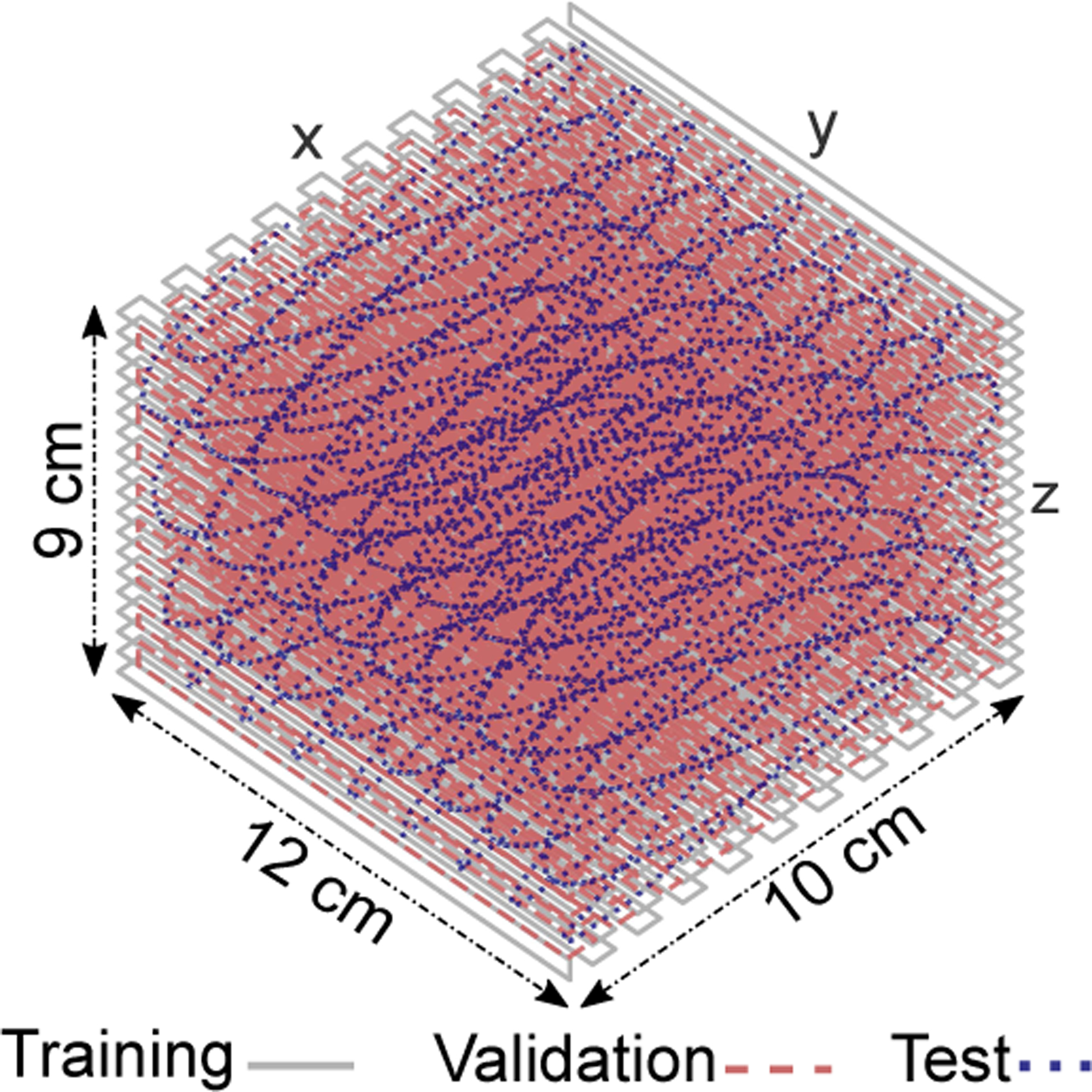
3D trajectories used to collect the training, validation and testing datasets.

The localization model $\widehat{f}$ is based on a feed-forward neural network with two hidden layers. The effectiveness of a feed-forward neural network is demonstrated in [8], and our preliminary research showed empirically that using two hidden layers provides a localization accuracy that is as good as with more than two layers but better than with only a single layer. The hyperparameters of the model are tuned using the validation dataset with learning rates selected from $\left\{0.0003,0.001,0.003\right\}$, the number of neurons in each hidden layer selected from $\left\{256,512,1024\right\}$, and the minibatch size selected from $\left\{16,64,128\right\}$. A grid search over these parameters is applied, where candidate models with different hyperparameter configurations are trained for 50 epochs. The model with the minimum validation loss is selected for testing. Mean squared error is selected as the loss function, Adam [21] is chosen as the optimizer, and PyTorch is used to generate the model [22].

C. Deployment Dataset

To evaluate the effect of magnetization, four deployment datasets were collected. A Wiha 40010 magnetizer/demagnetizer (Wiha Werkzeuge GmbH, Schonach, Germany) was used to induce random magnetization (i.e., different FoR) to the magnetometer between each dataset. To evaluate the performance of the model on a different magnetometer, two additional datasets were collected for which the magnetometer used to train the localization model is replaced by a different magnetometer. The training trajectory is purposely used for each of these six deployment datasets in order to emphasize the effects of change of magnetization/magnetometer on magnetic localization. During dataset collection, magnetometers were not rotated or exposed to magnetic interference.

D. Calibration Procedures

For EF, the magnetometer was rotated in different directions for 20 seconds and away from any magnet. The EF method detailed in [10] was used to transform the obtained ellipsoid into a sphere. Under the assumption that each magnetic measurement should have the same magnitude after a successful calibration, we first calculated the 5% and 95% percentiles of the magnitudes, denoted as $r_1$ and $r_2$. As a fitness score for this calibration, we used $\left(r_2-r_1\right)/\left(0.5\times \left(r_1+r_2\right)\right)$ to emphasize that magnitudes should be concentrated around a single value. If the fitness score was below an empirical value of 0.07, the calibration was considered successful and corresponding transformation matrix ${\mathbf{G}}^{\mathbf{E}\mathbf{F}}=\left[\begin{array}{c}{\mathbf{b}}^T\\ \mathbf{A}\end{array}\right]$ is returned.

For the PDIST, $D_T^Q$ and ${\tilde{D}}^Q$ were collected before their complete datasets. Although we used a 5D positioning stage in this proof-of-concept study, collecting these datasets can be completed by simply placing magnetometers into predetermined positions and recording magnetic measurements from those locations. It is important to state that during the data collections of $D_T^Q$ and ${\tilde{D}}^Q$, preserving magnet/magnetometer placements and orientations is vital for finding the correct transformation. $D_T^Q$ was used as the reference dataset to project the magnetic measurements of the deployment dataset onto the training's FoR through the mapping function ${\mathbf{G}}^{\text{PDIST}}$ using equation (2). Depending on the followed calibration strategy, we apply equation (3) using either ${\mathbf{G}}^{\mathbf{E}\mathbf{F}}$ or ${\mathbf{G}}^{\text{PDIST}}$ to transform $𝓓$.

IV. Results & Discussion

Positional errors are calculated using the $L_2$-norm of the difference between the 3D positions that were predicted by our localization model and the ground-truth provided by the positioning stage. The distribution of the positional errors are shown as box plots, and to facilitate the comparison of our results to other studies, the root mean squared error (RMSE), median error and the 75% quartile (Q3) error, are also provided in tables. The results have been validated for consistency by repeating the data collection with all possible combinations of training and deployment testing using three magnetometers. For brevity, only the results from one of the possible train/deployment combinations are reported.

A. Localization Accuracy After Training

Although the primary focus of this paper is on the differences in localization accuracy between the training and deployment datasets, the results corresponding to the validation and test datasets are still provided to emphasize that the trained model is indeed effective in predicting trajectories other than that of the training. Table I shows that the RMSE and median errors across all datasets are at or below 1 mm, while Q3 errors are between 1.3 mm and 1.6 mm, suggesting that the model generalizes well to the target volume as long as the current magnetization of the training magnetometer is preserved.

TABLE I.

Positional Errors of the trained model (in mm).

Dataset	RMSE	Median	Q3
Training $\left(D_T\right)$	0.78	0.89	1.34
Validation	0.75	0.84	1.29
Testing	0.86	1.02	1.54

B. Reliability Under Change in Magnetization

Fig. 5 shows more detailed results with $D_T$ denoting the training dataset and ${\tilde{D}}_1-{\tilde{D}}_4$ are the four deployment datasets collected by the same magnetometer but with different magnetizations. In Fig. 5a, the distribution shift is shown as the difference in magnetic measurement between $D_T$ and each deployment dataset. The effect of change in magnetization on the input space is significantly reduced when PDIST is used compared to EF. Indeed, the median differences of magnetic measurements with PDIST are consistently below 20 LSB, closer to the range of noise level of the magnetometer (mean: 10.57 LSB, std: 7.78 LSB), while being much larger with EF for ${\tilde{D}}_2-{\tilde{D}}_4$ (median > 50 LSB). Even though EF performed better on ${\tilde{D}}_1$, it remains worse than PDIST. In contrast, the results with PDIST are consistent throughout the four datasets.

Fig. 5.

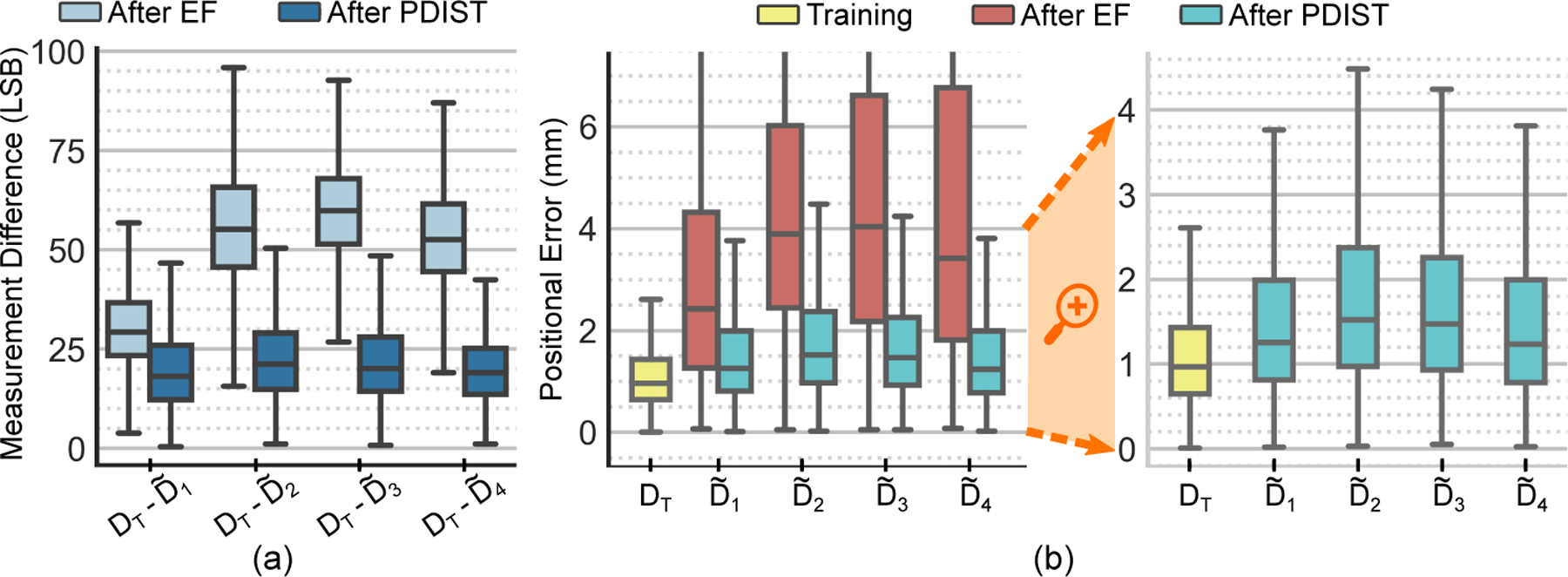
Effects of PDIST under change in magnetization. (a) Distribution of the norm of the magnetic measurement differences between training set and deployment sets. (b) Distribution of positional errors.

Box plots of the positional errors are shown in Fig. 5b. and Table II provides the error values for the median, Q3 and RMSE. With EF, the localization results show that even for measurements obtained from seen positions during training, the median errors vary significantly from 2–4 mm and Q3 from 4–7 mm which is not reasonable for many body motion tracking applications. With PDIST (Fig. 5c), the median errors are below 1.5 mm and Q3 errors are between 2–2.5 mm. Therefore, the positional errors are not only much lower with PDIST when compared to EF, but also more consistent across all deployment datasets which provides evidence that PDIST is a more reliable calibration method to mitigate the effect of magnetization.

TABLE II.

Positional Errors (in mm) Across Deployment Datasets with Change in Magnetization.

Dataset	RMSE		Median		Q3
	EF	PDIST	EF	PDIST	EF	PDIST
${\tilde{D}}_1$	2.09	1.12	2.43	1.26	4.33	1.99
${\tilde{D}}_2$	3.08	1.27	3.89	1.52	6.02	2.38
${\tilde{D}}_3$	3.15	1.19	4.04	1.48	6.63	2.26
${\tilde{D}}_4$	3.36	1.09	3.43	1.24	6.78	1.99

C. Reliability Under Change of Magnetometer

The results are shown in Fig. 6 for which ${\tilde{D}}_A$ and ${\tilde{D}}_B$ denote two deployment datasets collected by two magnetometers different than the one used for training $\left(D_T\right)$. For EF, the distribution drift between the input spaces (Fig. 6a) is more evident than in the previous data collection. It appears that EF has more difficulty with attenuating distribution drift from one magnetometer to another than reducing magnetization of a same magnetometer. Consequently, this is reflected on the localization accuracy (Fig 6b) that can reach a median error around 9 mm and a Q3 of 13 mm for ${\tilde{D}}_A$. The results with PDIST (Fig. 6c) is again much better with median errors remaining consistently around 1.2 mm and Q3 around 2 mm. The exact values of positional errors for RMSE, median, and Q3 are shown in Table III.

Fig. 6.

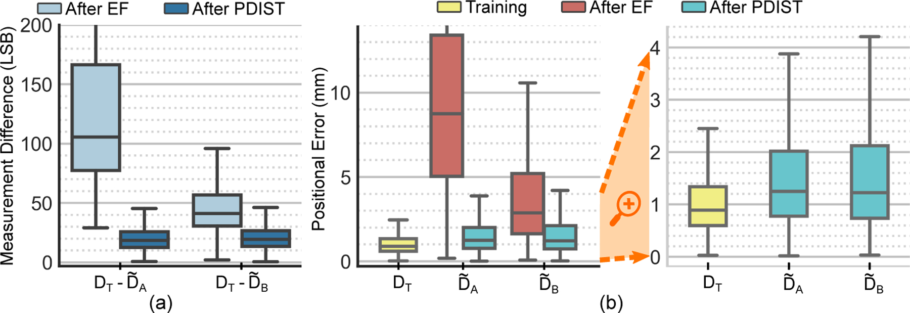
Effects of PDIST under change of magnetometer. (a) Distribution of the norm of the magnetic measurement differences between training set and deployment sets. (b) Distribution of positional errors.

TABLE III.

Positional Errors (in mm) Across Deployment Datasets with Changing Magnetometer.

Dataset	RMSE		Median		Q3
	EF	PDIST	EF	PDIST	EF	PDIST
${\tilde{D}}_{\mathbf{A}}$	5.61	1.18	8.76	1.25	13.42	2.02
${\tilde{D}}_B$	2.43	1.26	2.86	1.23	5.22	2.13

D. Analysis on Sampling for PDIST

The number of samples of $D^Q$ must be carefully selected for our PDIST to be practical. Indeed, the PDIST will be performed by end users before starting a tracking session. Obviously, they will not have access to a 3D positioning stage, nor have the time to collect a large and comprehensive $D^Q$. Therefore, the objective is to reach a sufficient level of reliability with the minimum number of samples. In the future, we are planning to develop a custom-designed calibration device in which the magnetometer can be placed by an end user in a small set of predefined positions to collect $D^Q$. Additionally, the locations of a fixed number of samples are important to maximize reliability. To assess the effect of number and locations of the $D^Q$ samples, we performed PDIST using the following strategies:

• a₁. 24 samples distributed across the volume

• a₂. 12 samples distributed across the volume

• a₃. 6 samples distributed across the volume

• a₄. 8 samples distributed across regions of higher magnetic strength (closer to the magnets)

• a₅. 8 samples distributed across regions of lower magnetic strength (away from the magnets)

These strategies were tested on all datasets, but for brevity, Fig. 7 is only showing the results for ${\tilde{D}}_1$, ${\tilde{D}}_2$, ${\tilde{D}}_{\mathbf{A}}$ and ${\tilde{D}}_B$.

Fig. 7.

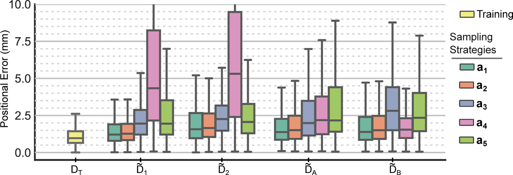
Effects of different sampling strategies for PDIST. Boxplots show the distributions of localization errors.

Overall, a₁ and a₂ have consistently the lowest localization errors across all datasets, except ${\tilde{D}}_B$ for which the difference with the best strategy (a₄) is not significant. Similar results to a₁ and a₂ are also shown for a₃, however, its poor tracking performance for ${\tilde{D}}_B$ might be significant enough to discard it as a suitable strategy. Regarding the region of sampling, it seems that a region with higher (a₄) or lower (a₅) magnetic field strength alone is not sufficient for PDIST to improve localization reliably. Indeed, higher localization errors are generally found for a₄ and a₅, and for ${\tilde{D}}_2$ with ${\mathbf{a}}_4$, the performance with PDIST is even worse than with EF. These results show that the region where the samples are collected is more important than the number of samples. Therefore, a₂ seems to be the best strategy to create ${𝓓}^Q$ because it has the best balance between localization error and sample size.

E. Sources of Error & Limitations

In this section, we discuss sources of errors which include noise, non-linearity and effects of orientation and magnetometer/magnet placements, and their effects on the performance of PDIST.

1). Noise:

The 5D positioning stage stopped at each predetermined PDIST location and recorded a sample before moving to the next location. Therefore, there was no noise due to motion artifacts. However, the magnetometer has its own electronic noise but was negligible to significantly distort measurements.

2). Orientation and magnetometer/magnet placements:

During our experiments, thanks to the 5D positioning stage, the locations and orientations of magnetometers/magnets remained fixed. It is of great importance to preserve this configuration across training and deployment in a practical application since differences in orientation might result in finding a wrong transformation between input spaces due to outliers and consequently cause higher localization errors. Future work will include creating a practical setup that will prevent such issues.

3). Non-linearity of transformation:

If the relationship between input spaces was only a shift or rotation, the location of the samples would not matter to find the linear transformation $\mathbf{G}$. However, our results suggest that the samples should be distributed throughout the volume, and thus implying that capturing samples in regions with different magnetic field strengths has an effect on the performance of PDIST. Therefore, together with the fact that PDIST is not completely removing the sources of unreliability since its positional errors in the deployment datasets are still higher than after training, this might indicate that the underlying transformation $\mathbf{G}$ could be non-linear. Future work will compare the performance of PDIST with non-linear transformations.

V. Conclusion

In this paper, we introduced the post-deployment input space transformation (PDIST) as a new magnetic calibration method that was designed to reduce the effect of distribution shift, and consequently improve localization reliability after the deployment of the localization model in the field. Unlike the conventional ellipsoid fit calibration, PDIST uses the information about the input space during the training of the localization model to offer superior reliability and accuracy post-deployment by projecting the magnetometer readings back to the input space used during training. Although PDIST requires a slightly longer calibration procedure than existing methods, future work will aim at improving this procedure for the end user by designing a more practical calibration setup that will consist of placing the magnetometer into a limited number of predetermined slots on a 2D plate. Furthermore, the localization results with PDIST were shown to be consistent across multiple datasets that were collected with changing magnetization and magnetometers, indicating that our localization method is reliable for practical usage. With this work, the objective is to enable researchers to have access to a wearable motion tracking system, including those in the field of speech research that are in a dire need of a wearable articulograph to track tongue motion to improve sound production [23].

References

- [1].Welch G and Foxlin E, “Motion tracking: No silver bullet, but a respectable arsenal,” IEEE Computer graphics and Applications, vol. 22, no. 6, pp. 24–38, 2002. [Google Scholar]
- [2].Zhou H and Hu H, “Human motion tracking for rehabilitation-a survey,” Biomedical signal processing and control, vol. 3, no. 1, pp. 118, 2008. [Google Scholar]
- [3].Filippeschi A, Schmitz N, Miezal M, Bleser G, Ruffaldi E, and Stricker D, “Survey of motion tracking methods based on inertial sensors: A focus on upper limb human motion,” Sensors, vol. 17, no. 6, p. 1257, 2017. [DOI] [PMC free article] [PubMed] [Google Scholar]
- [4].Sabatini AM, “Estimating three-dimensional orientation of human body parts by inertial/magnetic sensing,” Sensors, vol. 11, no. 2, pp. 1489–1525, 2011. [DOI] [PMC free article] [PubMed] [Google Scholar]
- [5].Menolotto M, Komaris D-S, Tedesco S, O'Flynn B, and Walsh M, “Motion capture technology in industrial applications: A systematic review,” Sensors, vol. 20, no. 19, p. 5687, 2020. [DOI] [PMC free article] [PubMed] [Google Scholar]
- [6].Sebkhi N, Bhavsar A, Anderson DV, Wang J, and Inan OT, “Inertial measurements for tongue motion tracking based on magnetic localization with orientation compensation,” IEEE sensors journal, vol. 21, no. 6, pp. 7964–7971, 2020. [DOI] [PMC free article] [PubMed] [Google Scholar]
- [7].Shahmiri F, Sebkhi N, Bhavsar A, Edwards WK, and Inan OT, “Joint angle measurements using magnetic sensing: A feasibility study,” in 2022 IEEE-EMBS International Conference on Wearable and Implantable Body Sensor Networks (BSN), pp. 1–4, IEEE, 2022. [Google Scholar]
- [8].Sebkhi N, Sahadat N, Hersek S, Bhavsar A, Siahpoushan S, Ghoovanloo M, and Inan OT, “A deep neural network-based permanent magnet localization for tongue tracking,” IEEE Sensors Journal, vol. 19, no. 20, pp. 9324–9331, 2019. [Google Scholar]
- [9].Ozyagcilar T, “Calibrating an ecompass in the presence of hard and soft-iron interference,” Freescale Semiconductor Ltd, pp. 1–17, 2012. [Google Scholar]
- [10].Cui X, Li Y, Wang Q, Zhang M, and Li J, “Three-axis magnetometer calibration based on optimal ellipsoidal fitting under constraint condition for pedestrian positioning system using foot-mounted inertial sensor/magnetometer,” in 2018 IEEE/ION Position, Location and Navigation Symposium (PLANS), pp. 166–174, 2018. [Google Scholar]
- [11].Chi C, Lv J-W, and Wang D, “Calibration of triaxial magnetometer with ellipsoid fitting method,” in IOP Conference Series: Earth and Environmental Science, vol. 237, p. 032015, IOP Publishing, 2019. [Google Scholar]
- [12].Kok M and Schön TB, “Magnetometer calibration using inertial sensors,” IEEE Sensors Journal, vol. 16, no. 14, pp. 5679–5689, 2016. [Google Scholar]
- [13].Kok M, Hol JD, Schön TB, Gustafsson F, and Luinge H, “Calibration of a magnetometer in combination with inertial sensors,” in 2012 15th International Conference on Information Fusion, pp. 787793, IEEE, 2012. [Google Scholar]
- [14].Ousaloo H, Sharifi G, Mahdian J, and Nodeh M, “Complete calibration of three-axis strapdown magnetometer in mounting frame, “IEEE Sensors Journal, vol. 17, no. 23, pp. 7886–7893, 2017. [Google Scholar]
- [15].Wu Y, Zou D, Liu P, and Yu W, “Dynamic magnetometer calibration and alignment to inertial sensors by kalman filtering,” IEEE Transactions on Control Systems Technology, vol. 26, no. 2, pp. 716–723, 2017. [Google Scholar]
- [16].Moreno-Torres JG, Raeder T, Alaiz-Rodríguez R, Chawla NV, and Herrera F, “A unifying view on dataset shift in classification,” Pattern recognition, vol. 45, no. 1, pp. 521–530, 2012. [Google Scholar]
- [17].Kull M and Flach P, “Patterns of dataset shift,” in First international workshop on learning over multiple contexts (LMCE) at ECML-PKDD, vol. 5, 2014. [Google Scholar]
- [18].Zhu M, Wu Y, and Yu W, “An efficient method for gyroscope-aided full magnetometer calibration,” IEEE Sensors Journal, vol. 19, no. 15, pp. 6355–6361, 2019. [Google Scholar]
- [19].Foster CC and Elkaim GH, “Extension of a two-step calibration methodology to include nonorthogonal sensor axes,” IEEE Transactions on Aerospace and Electronic Systems, vol. 44, no. 3, pp. 1070–1078, 2008. [Google Scholar]
- [20].Papafotis K and Sotiriadis PP, “Accelerometer and magnetometer joint calibration and axes alignment,” Technologies, vol. 8, no. 1, p. 11, 2020. [Google Scholar]
- [21].Kingma DP and Ba J, “Adam: A method for stochastic optimization,” arXiv preprint arXiv:1412.6980, 2014. [Google Scholar]
- [22].Paszke A, Gross S, Chintala S, Chanan G, Yang E, DeVito Z, Lin Z, Desmaison A, Antiga L, and Lerer A, “Automatic differentiation in pytorch,” 2017. [Google Scholar]
- [23].Cao B, Ravi S, Sebkhi N, Bhavsar A, Inan OT, Xu W, and Wang J, “Magtrack: A wearable tongue motion tracking system for silent speech interfaces,” Journal of Speech, Language, and Hearing Research, pp. 116, 2023. [DOI] [PMC free article] [PubMed] [Google Scholar]