Making Sense of Censored Covariates: Statistical Methods for Studies of Huntington’s Disease

Abstract

The landscape of survival analysis is constantly being revolutionized to answer biomedical challenges, most recently the statistical challenge of censored covariates rather than outcomes. There are many promising strategies to tackle censored covariates, including weighting, imputation, maximum likelihood, and Bayesian methods. Still, this is a relatively fresh area of research, different from the areas of censored outcomes (i.e., survival analysis) or missing covariates. In this review, we discuss the unique statistical challenges encountered when handling censored covariates and provide an in-depth review of existing methods designed to address those challenges. We emphasize each method’s relative strengths and weaknesses, providing recommendations to help investigators pinpoint the best approach to handling censored covariates in their data.

1. INTRODUCTION

More than 360 years ago, the field of survival analysis was born out of the seventeenth-century mortality studies of John Graunt and Edmond Halley, who were modeling time to death (i.e., survival). In the centuries since, survival analysis has expanded beyond modeling time to death and now encompasses modeling time to any event, such as time to cancer recurrence. Numerous statistical methods have been developed for survival (or time-to-event) analysis, and those methods have been adopted in actuarial science, biomedical studies, and engineering, just to name a few. Yet, all of these methods, and their applications, are for settings where the outcome in the statistical model is censored. Now, as biomedical challenges continue to revolutionize the landscape of survival analysis, a new modeling challenge has emerged: models where the covariate rather than the outcome is censored. While this challenge arises in a wide range of biomedical research areas from audiology to oncology, this article focuses on the context of studying disease-modifying therapies for neurodegenerative diseases (i.e., diseases that destroy neurons), like Huntington’s, Alzheimer’s, and Parkinson’s.

Neurodegenerative diseases lead to impairments in many aspects of life, including cognitive, motor, and daily function (e.g., paying bills). These impairments worsen slowly, often over decades, but the steepest change is expected in the period immediately before and after a clinical diagnosis. Since the neuron damage causing these impairments is irreversible, slowing the progression of these diseases is the objective of new experimental therapies. One notoriously difficult challenge with neurodegenerative diseases is identifying the optimal time to initiate therapies (Wild & Tabrizi 2017, Connor 2018, Dickey & La Spada 2018, Estevez-Fraga et al. 2020). Modeling how symptoms (i.e., impairments) worsen over time—the symptom trajectory—before and after clinical diagnosis can help identify that optimal time. These models can help pinpoint when best to initiate therapies that might delay a clinical diagnosis or slow the disease progression after a clinical diagnosis (Long et al. 2014, Epping et al. 2016, Scahill et al. 2020). Because they are anchored at clinical diagnosis (Figure 1), these symptom trajectories are modeled as functions of a time-to-event covariate, time to clinical diagnosis (hereafter, simply time to diagnosis).

Figure 1.

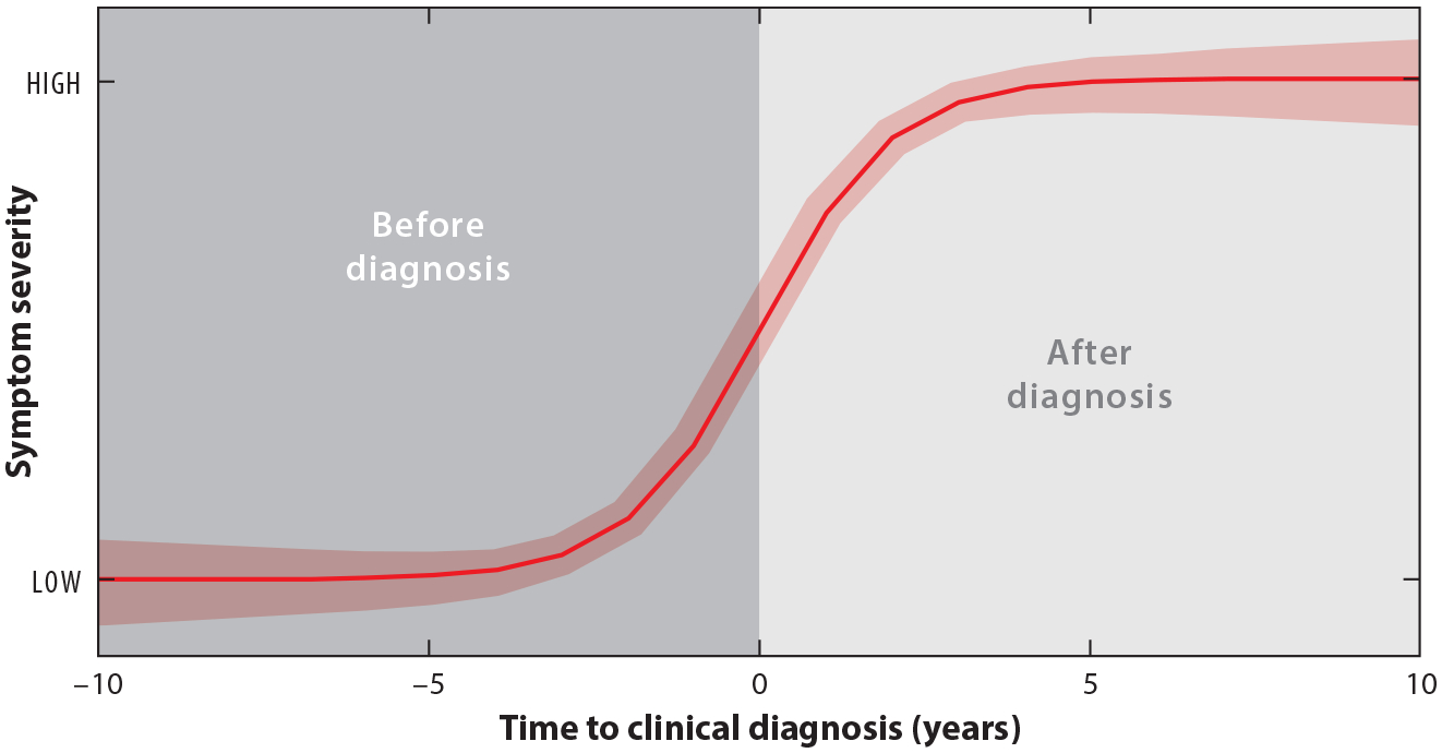
Hypothetical symptom trajectory as a function of time to diagnosis. Higher scores correspond to worse symptoms.

Modeling the symptom trajectory as a function of time to diagnosis is even challenging for Huntington’s disease, where researchers can track symptoms in patients who are guaranteed to develop the disease. All cases of Huntington’s disease are caused by a triplet repeat expansion of cytosine-adenine-guanine (CAG) in the HTT gene, so any patient with ≥36 CAG repeats will develop the disease with 100% certainty (Huntington’s Dis. Collab. Res. Group 1993). This genetic certainty is devastating but also offers hope. Through genetic testing, at-risk patients can be identified and recruited into observational studies, where researchers can track their symptom development in the pre- and postdiagnosis periods. A clinical diagnosis is made when motor abnormalities are unequivocal signs of Huntington’s disease (Huntington Study Group 1996). To date, there have been five such observational studies of Huntington’s disease, including more than 8,000 at-risk patients. Researchers can thus track and model symptoms for these patients as a function of time to diagnosis to determine when a therapy has the best chance of modifying the disease course. Yet, like other neurodegenerative diseases, Huntington’s disease progresses slowly over decades (Dutra et al. 2020), so these studies often end before a clinical diagnosis is made for everyone (Table 1). Thus, time to diagnosis is right-censored (i.e., a patient’s motor abnormalities will merit a clinical diagnosis sometime after the last study visit, but exactly when is unknown), leaving researchers with the challenge of modeling the symptom trajectory before and after clinical diagnosis without full information about when clinical diagnosis occurs.

Table 1.

Summary of patients from five observational studies of Huntington’s disease

	TRACK-HD	COHORT	PHAROS	PREDICT-HD	ENROLL-HD
Study duration	2008–2011 (4 years)	2005–2011 (7 years)	1999–2009 (11 years)	2002–2014 (13 years)	2012-Present (12+ years)
Sample size	257	1,326	356	1,159	5,173
% of patients who did not receive a clinical diagnosis during the study	85%	81%	82%	77%	88%

At study entry, all patients (a) had not been clinically diagnosed, (b) had CAG repeats ≥36, and (c) were ≥18 years old. Abbreviations: CAG, cytosine-adenine-guanine; COHORT, Cooperative Huntington Observational Research Trial; PHAROS, Prospective Huntington At Risk Observational Study; PREDICT-HD, Neurobiological Predictors of Huntington’s Disease.

The challenge creates a unique statistical problem of estimating the symptom trajectory as a function of a time-to-event covariate—time to diagnosis—that is right-censored (or, simply, a right-censored covariate). At first glance, a right-censored covariate may seem no different than a covariate with missing data, which, if true, means we could use well-established techniques for missing data (e.g., Little & Rubin 2002). Yet, censoring is different from missingness. With missingness, we have no information about the true covariate value. With censoring, we have partial information: If a patient was observed for 5 years and the study ended before a diagnosis was made, we know that their time to diagnosis was at least 5 years. Missing data techniques are not built to incorporate such partial information. That said, missing data techniques have inspired several methods to handle a censored covariate, many of which we explore in this review.

Whereas methods for time-to-event outcomes have been well-reviewed and well-documented in the literature (Schober & Vetter 2018, Seungyeoun & Heeju 2019, Turkson et al. 2021), the field of censored covariates is still in its infancy. This review aims to introduce methods that tackle the challenges of censored covariates in regression, often using an observational study of Huntington’s disease as an example to show how these methods are used in practice. Other examples are given to show that not all censored covariates are time-to-event covariates. We hope this review will inspire statisticians and nonstatisticians alike to incorporate and build upon the methods reviewed.

In Section 2, we establish the statistical building blocks for a censored covariate. In Section 3, we discuss current attempts to repurpose traditional survival analysis methods to handle covariate censoring. In Section 4, we examine the consequences of simple, albeit ill-advised, methods to handle covariate censoring. Thereafter, we focus on the advantages and disadvantages of other methods: a complete case analysis (Section 5), weighting methods (Section 6), imputation methods (Section 7), likelihood methods (Section 8), Bayesian methods (Section 9), and threshold methods (Section 10). Lastly, in Section 11, we cover possible directions for future work.

2. BUILDING BLOCKS

2.1. Notation

To set the stage for handling a censored covariate, we start with a regression model with a censored covariate. Let $Y$ be a continuous outcome, $X$ be a censored covariate, and $\mathit{Z}$ be a $p\times 1$ vector of fully observed covariates. Our model is

$$Y=m(X,\mathbf{Z};\mathit{\beta })+ϵ,$$ 1.

where the mean function $m(\cdot )$ can be any linear or nonlinear function, and the random errors $ϵ$ are assumed to be normally distributed with mean zero and variance ${\sigma }^2$. The errors $ϵ$ are also assumed to be independent of the covariates $(X,\mathit{Z})$.

In Huntington’s disease research, this model could be used to assess how symptoms change over the course of a study as a function of time to diagnosis and other patient characteristics (Abeyasinghe et al. 2021). Huntington’s disease symptoms can be quantified by the composite Unified Huntington’s Disease Rating Scale (cUHDRS), which measures motor, cognitive, and daily function (Schobel et al. 2017). We can use Equation 1 to model changes in cUHDRS from the beginning to the end of a study $\left(Y\right)$ as a function of time to diagnosis $(A-X)$, where $A$ and $X$ are ages at study entry and clinical diagnosis, respectively, and other patient characteristics like the number of CAG repeats $\left(\mathit{U}\right)$. Here, $\mathit{Z}={\left(A,{\mathit{U}}^{\text{T}}\right)}^{\text{T}}$.

Our main goal is to obtain consistent estimates for $\mathit{\theta }={\left({\mathit{\beta }}^{\text{T}},{\sigma }^2\right)}^{\text{T}}$. However, because of censoring, the covariate $X$ is not fully observed. Instead, an observed covariate $W$ and an event indicator $\Delta$ are observed in place of $X$. Definitions of $W$ and $\Delta$ depend on the type of covariate censoring.

2.2. Types of Covariate Censoring

The types of covariate censoring include whether it is right, left, or interval censoring and whether the censoring is random or nonrandom.

2.2.1. Right, left, or interval censoring.

Right censoring happens in Huntington’s disease studies, for example, when the study ends or a patient leaves the study before a clinical diagnosis is made. A patient’s true, but unobserved, age at clinical diagnosis $\left(X\right)$ is known to lie after their age at last study visit $\left(C\right)$. We observe $W=\text{min}(X,C)$ and $\Delta =\text{I}(X\le C)$.

Left censoring happens in Huntington’s disease studies, for example, when a patient joins the study after a clinical diagnosis was already made but at an unknown time. A patient’s true, but unobserved, age at clinical diagnosis $\left(X\right)$ is known to lie before the patient’s age at first study visit $\left(C\right)$. We observe $W=\text{max}(X,C)$ and $\Delta =\text{I}(C\le X)$.

Interval censoring happens in Huntington’s disease studies, for example, when a patient meets the criteria for a clinical diagnosis between two study visits. A patient’s true, but unobserved, age at clinical diagnosis $\left(X\right)$ is known to lie between their ages at last prediagnosis visit $\left(C_1\right)$ and first postdiagnosis visit $\left(C_2\right)$. We observe $W_1=\text{min}\left(X,C_1\right),W_2=\text{max}\left(X,C_2\right)$, and $\Delta =\text{I}\left(C_1<X\le C_2\right)$.

2.2.2. Nonrandom or random censoring.

Nonrandom censoring, or type I censoring, is when the censoring values (e.g., $C$) are constants known in advance. For example, Huntington’s disease researchers may want to evaluate changes in cUHDRS scores as a function of time to diagnosis, but only follow patients to age 50 since most patients are clinically diagnosed by that time (Roos 2010). Researchers could thus recruit at-risk patients who are under 50 years old, track them until age 50, and then drop them from the study once they are older than 50. Any patient who had not met the criteria for clinical diagnosis by age 50 would have an age at diagnosis that is right-censored by fixed $C=50$.

A special type of nonrandom censoring is limit of detection censoring, where a covariate $X$ is censored if it lies above or below a certain (fixed) detection level, typically determined by the limitations of instruments used to take measurements. For example, limit of detection censoring happens in Huntington’s disease studies when quantifying the severity of tremors with accelerometers, which is a limit-of-detection-censored covariate since accelerometers can only measure severity within a certain range. (Notice from this example that censored covariates do not have to be times to events.) Until about 2017, the censored covariate literature focused mainly on limit of detection censoring (e.g., Bernhardt et al. 2015, Kong & Nan 2016, Sattar & Sinha 2017).

Random censoring is when the censoring values (e.g., $C$) are not set constants and thus not known in advance. For Huntington’s disease, random censoring of age at clinical diagnosis occurs, for example, when the study ends due to discontinued funding. Any patient still undiagnosed when the funding stopped would have an age at diagnosis that is right-censored by a random $C$ being their age at last visit before the funding stopped.

A special case of random censoring is type II censoring, which occurs when a study is stopped after a prespecified number of events have occurred (Schneider & Weissfeld 1986). For example, in a Huntington’s disease study, type II censoring occurs if the study is stopped after, say, 30 patients have met the criteria for a clinical diagnosis. Other patients still undiagnosed when the study stopped will have an age at diagnosis that is censored by a random $C$ being their age when the study ended.

2.2.3. Summary.

When handling censored covariates, it is important to know whether we have right, left, or interval censoring to interpret what variables are observed in place of $X$ (i.e., $W$ and $\Delta$). It is also important to know whether the censoring is nonrandom or random to determine if a probability distribution must be assigned to the censoring variable. When censoring is nonrandom, a probability distribution is not needed; when censoring is random, it is needed.

2.3. Assumptions and Identification

Unless mentioned otherwise, the remainder of this review focuses on statistical methods to estimate the parameters $\mathit{\theta }$ in the model in Equation 1 under the following four assumptions. (a) We assume $X$ is a right-censored covariate and $C$ is a random censoring value. (b) We assume that $X$ is independent of $C$, an assumption known as noninformative censoring. Noninformative censoring is typically assumed in Huntington’s disease studies, since the reason censoring occurs has nothing to do with a patient’s illness. (c) We assume $Y$ is independent of $C$ given $X$, so that information about $C$ is superfluous when $X$ is observed. (d) Lastly, we assume $m(X,\mathit{Z};\mathit{\theta })$ is weakly increasing in $X$, an assumption used for identifiability of $\mathit{\theta }$.

Under these assumptions, $\mathit{\theta }$ is identifiable. Let the conditional density for $X$ given $\mathit{Z}$ be denoted by $f_{X\mid \mathit{Z}}(x,\mathit{z})$. When $f_{X\mid \mathit{Z}}(x,\mathit{z})$ is known and parametric, Hsiao (1983) proved $\mathit{\theta }$ is identifiable with only assumptions (a)–(c). When $f_{X\mid \mathit{Z}}(x,\mathit{z})$ is unknown, Manski & Tamer (2002) proved $\mathit{\theta }$ is identifiable under assumptions (a)–(d).

3. REVERSE SURVIVAL REGRESSION

The literature on methods to handle censored outcomes is well-developed, which raises the following question: Can we take advantage of the existing methods for censored outcomes to develop methods for censored covariates? Atem and colleagues (Atem et al. 2016, 2017a; Qian et al. 2018) explored this idea using what they call reverse survival regression for a right-censored covariate in linear and logistic regression models. The roles of $Y$ and $X$ are reversed in the model so that $X$ can be treated as a right-censored outcome and $Y$ as a fully observed (continuous or binary) covariate.

This role reversal allows for the use of classic survival analysis techniques like the Cox proportional hazards model, are designed for right-censored outcomes. Atem and colleagues showed that reverse survival regression leads to accurate tests of association between $X$ and $Y$, controlling for $\mathit{Z}$. In fact, Atem et al. (2017a) proved that the test of association using the reversed Cox model where $X$ is the right-censored outcome and $Y$ is the covariate leads to the same conclusion as the test using the original model, where $X$ is the right-censored covariate and $Y$ is the outcome. However, if parameter estimation is of interest, reverse survival regression may not provide the needed answers. The parameter estimates from the fitted and intended models will not be the same (Atem et al. 2016).

Still, reverse survival regression has, so far, been shown to work well in testing associations between $X$ and $Y$ while controlling for $\mathit{Z}$ when (a) $Y$ is continuous, making the original model a linear regression model (Atem et al. 2017a, Qian et al. 2018) and (b) $Y$ is binary, making the original model a logistic regression model (Atem et al. 2016). It is unclear from the current literature whether the approach could extend to other models, such as a nonlinear mean model, but a proof for more general models could build on those currently used in reverse survival regression.

4. AD HOC METHODS WITHOUT GUARANTEES

4.1. Naive Analysis

Perhaps the simplest way forward would be to ignore covariate censoring and analyze the data by treating the observed $\mathit{\text{Ws}}$ as if they were the true $\mathit{\text{Xs}}$. This approach, known as naive analysis, is straightforward to implement with existing software; Table 2 shows how to apply a naive analysis to the model in Equation 1. Yet, a naive analysis estimates a completely different model than intended. Despite intending to capture the associations of $Y$ with $(X,\mathit{Z})$, the naive analysis actually captures $Y$’s associations with $(W,\mathit{Z})$. We discuss below how a naive analysis almost always leads to bias (e.g., Austin & Hoch 2004) and inflated type I error rates (e.g., Austin & Brunner 2003) when estimating and testing model parameters. Existing works have explored the problems with naive analysis under limit of detection censoring (e.g., Austin & Hoch 2004, Rigobon & Stoker 2009), and we include a brief simulation study to show similar problems under random censoring for a linear regression model (Supplemental Appendix A). Note that the naive analysis is difficult to apply with interval censoring, since it is not clear which of the observed values, $W_1$ or $W_2$, to treat as the true $X$.

Table 2.

Methods to estimate parameters $\theta$ in the regression model Equation 1 with a right-censored covariate when $X$ is independent of $C$ given $Z$

Method	Estimating equation or technique to solve for $\mathit{\theta }$
Naive analysis	${\sum }_{i=1}^n{𝒮}_{\mathit{\theta }}^F\left(y_i,w_i,{\mathit{z}}_i\right)=\mathbf{0}$
Substitution	${\sum }_{i=1}^n{𝒮}_{\mathit{\theta }}^F\left\{y_i,g\left(c_i\right),{\mathit{z}}_i\right\}=\mathbf{0}$
Complete case	${\sum }_{i=1}^n{\delta }_i{𝒮}_{\mathit{\theta }}^F\left(y_i,x_i,{\mathit{z}}_i\right)=\mathbf{0}$
IPW	${\sum }_{i=1}^n{\delta }_i{𝒮}_{\mathit{\theta }}^F\left(y_i,x_i,{\mathit{z}}_i\right)/\text{pr}\left(C\ge x_i\mid {\mathit{z}}_i\right)=\mathbf{0}$
AIPW	${\sum }_{i=1}^n{\delta }_i{𝒮}_{\mathit{\theta }}^F\left(y_i,x_i,{\mathit{z}}_i\right)/\text{pr}\left(C\ge x_i\mid {\mathit{z}}_i\right)+{\sum }_{i=1}^n\left\{1-{\delta }_i/\text{pr}\left(C\ge x_i\mid {\mathit{z}}_i\right)\right\}E\left\{{𝒮}_{\mathit{\theta }}^F(y,X,\mathit{z})\mid {\delta }_i=1,y_i,{\mathit{z}}_i\right\}=\mathbf{0}$
Imputationa	${\sum }_{i=1}^n\left[{\delta }_i{𝒮}_{\mathit{\theta }}^F\left(y_i,x_i,{\mathit{z}}_i\right)+\left(1-{\delta }_i\right){𝒮}_{\mathit{\theta }}^F\left\{y_i,E\left(X_i\mid X_i>c_i,{\mathit{z}}_i\right),{\mathit{z}}_i\right\}\right]=\mathbf{0}$
MLE	${\sum }_{i=1}^n\left[{\delta }_i{𝒮}_{\mathit{\theta }}^F\left(y_i,x_i,{\mathit{z}}_i\right)+\left(1-{\delta }_i\right)E\left\{{𝒮}_{\mathit{\theta }}^F\left(y_i,X_i,{\mathit{z}}_i\right)\mid {\delta }_i=0,y_i,c_i,{\mathit{z}}_i\right\}\right]=\mathbf{0}$
Bayesian	Use WinBugs or STAN for parameter estimation.
Deletion thresholdb	${\sum }_{i=1}^n{𝒮}_{\mathit{\theta }}^F\left(y_i,x_i^{*},{\mathit{z}}_i\right)=\mathbf{0}$
Complete thresholdb	${\sum }_{i=1}^n{𝒮}_{\mathit{\theta }}^F\left(y_i,w_i^{*},{\mathit{z}}_i\right)=\mathbf{0}$

Throughout, ${𝒮}_{\mathit{\theta }}^F(y,x,\mathit{z})=\partial \text{log}{f}_{Y\mid X,\mathit{Z}}(y,x,\mathit{z};\mathit{\theta })/\partial \mathit{\theta }$ denotes the score function. The function $f_{Y\mid X,\mathit{Z}}(y,x,\mathit{z};\mathit{\theta })$ is the conditional density of $Y$ given $(X,\mathit{Z})$ evaluated at $Y=y,X=x,Z=z$. Standard errors for all methods, except Bayesian, can be obtained using a sandwich estimator.

Abbreviations: AIPW, augmented inverse probability weighting; IPW, inverse probability weighting; MLE, maximum likelihood estimator.

^aThe imputation method shown corresponds to using the imputed value $\text{E}(X\mid X>c,\mathit{z})$. Options listed in Section 7.1 could be used instead.

^bSee Section 10 for how $x^{*}$ and $w^{*}$ are defined.

4.1.1. Biased estimation.

The naive analysis is almost always biased for the coefficient of censored $X$, but the direction of this bias depends on the type of covariate censoring. In settings of right or left limit of detection censoring, the naive analysis overestimates the coefficient of the censored covariate (Austin & Brunner 2003, Austin & Hoch 2004). This overestimation was dubbed expansion bias by Rigobon & Stoker (2009) for the following reason. For any covariate that is censored, we will observe a $W$ equal to the fixed constant $C$ since censoring is nonrandom. When there is substantial censoring, the data will contain many replicates of the same $W$ for all censored observations, creating a pileup at that value. That pileup will lead to overestimating the coefficient of $W$ with a naive analysis; the overestimation is expansion bias.

When covariate censoring is random, there is no pileup at a common $W$ value because each observation can be censored at different (random) times; each censored observation can have a unique $W$. Without the pileup at one $W$ value, the direction of the bias from a naive analysis depends on the direction of censoring (i.e., right or left censoring). In simulation studies, when a covariate is right- or left-censored, a naive analysis tends to over- or underestimate the coefficient values of censored $X$, respectively (Supplemental Figures 1 and 2).

We might expect that estimates of the coefficients for fully observed covariates $\mathit{Z}$ would be safe from the woes of a naive analysis, but this is not the case. The bias can bleed over into the model intercept and coefficients for the other fully observed covariates $\mathit{Z}$—if they are correlated with $X$—as well. Only when $\mathit{Z}$ are completely uncorrelated with $X$ will the naive analysis be unbiased for these coefficients. In simulation studies, we found that under limit of detection censoring for a linear regression model, the intercept is underestimated regardless of the correlation between $X$ and $\mathit{Z}$ (Supplemental Figures 3 and 4), but under random censoring, the intercept could be over- or underestimated (Supplemental Figures 1 and 2). Our simulation studies further showed that the coefficients of $\mathit{Z}$ were overestimated more under right censoring than left censoring (whether random or limit of detection).

4.1.2. Inflated type I error rates.

With its biased estimation, it is perhaps unsurprising that the naive analysis can also lead to incorrect statistical inference. A naive analysis can lead to inflated type I error rates (e.g., larger than 5%). In simulation studies, Austin & Brunner (2003) showed what can happen to the type I error rates in a linear regression model where a limit-of-detection-censored covariate $X$ is correlated with the outcome $Y$ and also with a single uncensored covariate $Z$, but $Z$ and $Y$ are independent. Despite $Z$ being uncensored and uncorrelated with $Y$, hypothesis tests of its coefficients had type I error rates significantly higher than the nominal 5%. Furthermore, the type I error rates increased (a) as the censoring rate increased, (b) as the magnitude of the coefficient of $X$ increased, (c) as the correlation between $X$ and $Z$ increased, and, counterintuitively, (d) as the sample size increased. Similarly, hypothesis tests of the coefficient of $X$, but not of $Z$, will have inflated type I error rates if $X$ is independent of both $Z$ and $Y$. Though we did not conduct a simulation study for type I error rates, we expect them to be inflated even when covariate censoring is random, given that the naive analysis also produces bias in that case. As the name suggests and empirical results confirm, a naive analysis is never recommended; we should never ignore covariate censoring in our data.

4.2. Substitution

Rather than ignore covariate censoring, one could adjust for it using a method known as substitution. With substitution, an analyst replaces any covariate that is censored with a simple guess for what that covariate value could be. For example, in Huntington’s disease studies, when a patient’s age at clinical diagnosis $X$ is censored, one could substitute for $X$ the average age of clinical diagnosis [i.e., 40 years old, (Duyao et al. 1993)].

The main appeal of substitution is its ease of implementation. Rather than requiring complicated modeling, censored covariates are replaced by a simple guess or some function of the censored value $g\left(C\right)$ to create a dataset that no longer has any censored values. This dataset can then be directly analyzed using any standard statistical software (see Table 2). However, substitution shares many of the same drawbacks as the naive analysis. In particular, substitution has no theoretical underpinnings, and numerous simulation studies have shown that it leads to bias for the coefficient of the censored covariate, with the magnitude of bias depending on the censoring rate and how close the substituted value is to the truth (Schisterman et al. 2006, Nie et al. 2010, Atem & Matsouaka 2017, Atem et al. 2017a). In short, neither the naive analysis nor the substitution method is advisable when handling a censored covariate. The remainder of this review discusses methods that better handle covariate censoring.

5. COMPLETE CASE ANALYSIS

A natural way to analyze censored covariate data is with a so-called complete case analysis, which involves analyzing the subset of the data that were not censored; that is, delete any observations where $\Delta \ne 1$ (Little 1992, Lv et al. 2017). This deletion yields a smaller, complete dataset. Deleting data is typically a faux pas in statistics due to the loss of efficiency that comes with it. Still, under certain conditions, using a complete case analysis to handle covariate censoring does lead to a consistent, albeit inefficient, estimator for model parameters.

5.1. Conditions for Consistency

The following conditions have been considered when using a complete case analysis to handle a right-censored covariate. Throughout, $⫫$; denotes independence between random variables. References listed refer to papers that used these conditions.

1. Exogenous censoring: $\text{E}(ϵ\mid \Delta ,X,\mathit{Z})=0$ (Rigobon & Stoker 2007, Tsimikas et al. 2012, Wang & Feng 2012)

2. Strict exogenous censoring: $ϵ⫫\Delta \mid (X,\mathit{Z})$ (Rigobon & Stoker 2007)

3. Conditionally independent censoring given $(X,\mathit{Z}):C⫫Y\mid (X,\mathit{Z})$ (Atem et al. 2016, 2017a; Lv et al. 2017; Qian et al. 2018)

4. Conditionally independent censoring given $\mathit{Z}:C⫫(X,Y)\mid \mathit{Z}$ (Atem et al. 2017b, Kong et al. 2018)

5. Independent censoring: $C⫫(Y,X,\mathit{Z})$ (Matsouaka & Atem 2020)

Although they are not equivalent, these conditions have a unidirectional hierarchy (Ashner & Garcia 2023). The weakest sufficient assumption in the hierarchy, condition 1 (exogenous censoring), leads to a consistent estimator when using a complete case analysis. Thus, whenever any of conditions 1–5 hold, the estimator from a complete case analysis (Table 2) will be consistent. For examples of how these conditions come up in studies of Huntington’s disease, readers are directed to Ashner & Garcia (2023).

Another way to summarize this result is that the complete case analysis will yield a consistent estimator as long as the outcome $Y$ is conditionally independent of one of the censoring variables ($C$ or $\Delta$), given covariates $(X,\mathit{Z})$. This condition is analogous to the one needed to ensure that a complete case analysis yields a consistent estimator when the covariate has missing data (Little 1992). Additionally, this condition sheds light on why we cannot use a complete case analysis in traditional survival analysis, where the outcome, rather than the covariate, is censored. Consistency is not guaranteed in that case because the censoring indicator $\Delta$ always depends on the censored outcome $Y$ [i.e., $\Delta =\text{I}(Y\le C)$]. This result highlights a stark contrast between censored covariates and censored outcomes: A complete case analysis can yield a consistent estimator for the former, but never for the latter (Bernhardt et al. 2015).

5.2. Considerations with the Complete Case Analysis

While the complete case analysis can offer consistency, we do not advocate for it as the default method. Because a complete case analysis deletes censored observations, it will suffer from information loss and statistical inefficiency. This problem is particularly concerning when censoring rates are large (like the 77%+ we see in Huntington’s disease observational studies) or sample sizes are small. Still, knowing when the complete case analysis yields a consistent estimator is helpful, as that knowledge can be used (a) to produce initial estimates for more complicated iterative estimation procedures, like some multiple imputation techniques (Bernhardt et al. 2014, Atem et al. 2016) or (b) as a baseline to demonstrate the efficiency gains of newer approaches (e.g., Bernhardt 2018, Matsouaka & Atem 2020). To the best of our knowledge, the unidirectional hierarchy between conditions 1–5 has only been established for a right-censored covariate. Analogous results for when the covariate is left- or interval-censored remain to be established.

6. WEIGHTING METHODS

6.1. Inverse Probability Weighting

When the subset of uncensored data is not representative of the whole sample, the complete case analysis is not appropriate. For a regression model with a right-censored covariate, inverse probability weighting (IPW) inversely weights each uncensored observation with the conditional probability of $X$ being uncensored given $\mathit{Z}$. The result is a weighted sample of the complete data that better represents the data we would have had without censoring.

A key component of IPW is estimating the weights, $\pi (x,\mathit{z})\equiv 1/\text{Pr}(C\ge x\mid \mathit{z})$, as these weights affect the variability (i.e., efficiency) of the estimated model parameters. Typical choices include estimating $\text{Pr}(C\ge x\mid \mathbf{z})$ parametrically (e.g., with logistic regression), semiparametrically (e.g., with Cox regression), and nonparametrically (e.g., with a Kaplan–Meier estimator) (Matsouaka & Atem 2020). An analyst must pay special attention to situations where $\text{Pr}(C\ge x\mid \mathit{z})$ is close to zero, in which case the weights, $1/\text{Pr}(C\ge x\mid \mathit{z})$, will blow up. These large weights can lead to situations where solving the IPW estimating equation in Table 2 is not possible due to nonconvergence or the resulting estimates of the model parameters having high variability. One way to counteract this problem is to use stabilized weights: Rather than use weight $\pi \left(x_i,{\mathit{z}}_i\right)$ for the $i$th observation, use $\pi \left(x_i,{\mathit{z}}_i\right)/{\sum }_{i=1}^n\pi \left(x_i,{\mathit{z}}_i\right)$, where $n$ is the sample size (Hernán & Robins 2010, Matsouaka & Atem 2020). The stabilized weights help to reduce the chance of the weights blowing up.

Like the complete case estimator, IPW will yield a consistent estimator for the model parameters when the outcome $Y$ is independent of the censoring $C$ (Matsouaka & Atem 2020). When $C$ depends on $Y$, but $C$ and $X$ are independent given $(Y,\mathit{Z})$, Lv et al. (2017) proved that IPW will yield a consistent estimator of the model parameters as long as the weights incorporate $Y$ and $\mathit{Z}$, i.e., the weights are $1/\text{Pr}(C\ge x\mid y,\mathit{z})$. Although it offers consistency in more settings than the complete case analysis, IPW has similar efficiency since observations are still being deleted.

6.2. Augmented Inverse Probability Weighting

One way to counteract the inefficiency from IPW is to use augmented inverse probability weighting (AIPW) (Seaman & White 2013). AIPW can be seen as a hybrid between (a) IPW (Section 6.1), which requires the conditional distribution of $C$ given $\mathit{Z}$, and (b) imputation (Section 7), which requires the conditional distribution of $X$ given $\mathit{Z}$.

AIPW is commonly applied in missing data settings, where, when data are missing at random (i.e., the missingness mechanism is independent of the missing value), the approach is known to be doubly robust. This property means that the AIPW estimator is consistent if at least one of the two models (i.e., the model for $C$ given $\mathit{Z}$ or for $X$ given $\mathit{Z}$) is correctly specified (Seaman & White 2013). However, the missing at random assumption does not apply to right-censored covariates because the censoring indicator $\Delta =\text{I}(X\le C)$ inherently depends on the censored covariate $X$. This violation means that the double robustness of AIPW may not be guaranteed for censored covariates if used directly, as it was developed for missing covariates (see Table 2 for the missing data version of AIPW applied to a regression model with a right-censored covariate).

To the best of our knowledge, Ahn et al. (2018) are, so far, the only ones to adapt AIPW to a censored covariate setting. Rather than using the AIPW estimating equations that were derived for missing data, Ahn et al. (2018) use semiparametric techniques (for more details, see Tsiatis 2006) to derive the appropriate estimating equations for their setting. Ahn et al. (2018) were then able to prove that, in their setting, their AIPW estimator maintains the doubly robust property that is expected from this technique.

6.3. Considerations with Weighting Methods

IPW and its augmented form have been applied to censored covariates (e.g., Ahn et al. 2018, Matsouaka & Atem 2020), but the methods have not been as commonly adopted as they have been for missing covariates. Both weighting methods offer consistency, and of the two, AIPW produces estimates with higher efficiency. Yet, so far, the typical double robustness of AIPW has only been demonstrated in one setting, and whether that double robustness property holds for other models and other covariate censoring types remains to be explored.

7. IMPUTATION METHODS

Another promising method motivated by the missing data literature is imputing, or filling in, the value for a right-censored covariate. Typically, imputation methods capture more information than the complete case analysis and offer better precision than weighting methods (Seaman & White 2013). Imputation methods proceed in two stages: imputation and analysis. While the analysis used in the second stage does not dictate how we impute data in the first, the quality of the imputed values does dictate how well the model parameters are estimated in the analysis.

7.1. Choosing the Imputed Values

A right-censored covariate is accompanied by partial information (i.e., that $X>C$) that a missing covariate does not have. To be valid for $X$, the imputed value should uphold this inequality (i.e., be $>C$). The conditional mean of $X$ given some observed data is commonly used as an imputed value. We discuss the most common conditional means, ordered by how much partial information about $X$ they incorporate, from least to most.

1. $\text{E}(X\mid \mathit{Z})$: This quantity is often used in studies of Huntington’s disease to impute right-censored ages at clinical diagnosis $\left(X\right)$; the imputed values are estimates of what the age at clinical diagnosis would be based on the patient’s current age and number of CAG repeats ($\mathit{Z}$) (Williams et al. 2015, Epping et al. 2016, Scahill et al. 2020). However, $\text{E}(X\mid \mathit{Z})$ includes no partial information from the censoring, and there are no guarantees that it will be valid (i.e., larger than the censored value $C$). For this reason, imputing with $\text{E}(X\mid \mathit{Z})$ is not guaranteed to yield a consistent estimator for the model parameters.

2. $\text{E}(X\mid C,\mathit{Z})$: This quantity incorporates the magnitude of $C$ but not the directional relationship between $X$ and $C$. Imputing censored $X$ with $\text{E}(X\mid C,\mathit{Z})$ (e.g., Geskus 2001) is actually an application of regression calibration (Prentice 1982). Still, there are no guarantees that the imputed $\text{E}(X\mid C,\mathit{Z})$ will be larger than $C$, so consistency in estimating the model parameters is not guaranteed.

3. $\text{E}(X\mid X>C)$: This quantity captures the partial information from right censoring (i.e., $X>C$) but omits any additional covariates $\mathit{Z}$, so all people censored at the same time would have the same imputed value (Richardson & Ciampi 2003; Schisterman et al. 2006; Nie et al. 2010; Arunajadai & Rauh 2012; Atem et al. 2017a,b, 2019; Wang et al. 2022). Nie et al. (2010) showed that imputing with $\text{E}(X\mid X>C)$ will yield a consistent estimator for the regression model parameters when the model is linear and the correct distribution is assumed for $X$. Still, because covariates $\mathit{Z}$ can be informative, Wang et al. (2022) proposed a two-stage approach that first imputes any right-censored $X$ with $\text{E}(X\mid X>C)$ and then updates the imputed values to incorporate information from $\mathit{Z}$ using machine learning methods. However, this second step reintroduces the possibility that the updated imputed values will not be valid.

4. $\text{E}(X\mid X>C,\mathit{Z})$: This quantity captures the partial information from right censoring (i.e., $X>C$) and the additional covariates $\mathit{Z}$, so people censored at the same time with different covariates can have different imputed values (Bernhardt et al. 2014, 2015; Atem et al. 2017b, 2019). Bernhardt et al. (2015) proved that imputing with $\text{E}(X\mid X>C,\mathit{Z})$ will yield a consistent estimator for parameters in a regression model when the model is linear and the correct conditional distribution for $X$ given $\mathit{Z}$ is used.

5. $\text{E}(X\mid X>C,\mathit{Z},Y)$: This quantity, which further conditions on $Y$, leads to improper imputation because our overarching goal is to estimate the relationship between $Y$ and $(X,\mathit{Z})$, but computing $\text{E}(X\mid X>C,\mathit{Z},Y)$ will use the opposite—or improper—relationship between $X$ and $(\mathit{Z},Y)$ (Bernhardt et al. 2015, Atem et al. 2017b). Still, adjusting for $Y$ makes sense when $X$ is somehow related to $Y$, as with Huntington’s disease, where the symptom severity $\left(Y\right)$ can influence when a patient gets clinically diagnosed $\left(X\right)$. Bernhardt et al. (2015) proved that imputing with $\text{E}(X\mid X>C,\mathit{Z},Y)$ will yield a consistent estimator for regression model parameters when the model is linear, the correct conditional distribution of $X$ given $\mathit{Z}$ and $Y$ is used, and $Y$ is conditionally independent of $X$ given $\mathit{Z}$.

Note that different imputed values are needed when $X$ is left- or interval-censored. For example, instead of conditional mean 4, we would have $\text{E}(X\mid X<C,\mathit{Z})$ when $X$ is left-censored and $\text{E}\left(X\mid C_1<X\le C_2,\mathit{Z}\right)$ when $X$ is interval-censored. Similar changes apply to the other conditional means.

There are other options to impute a right-censored $X$ besides the conditional means. One option is to impute using conditional quantiles based on a quantile regression of $X$ given $\mathit{Z}$ (Wang & Feng 2012). Estimates of the conditional mean can be sensitive to outliers in the data, so using a conditional quantile provides robustness to those outliers. A second option is a single index model, which imputes using $\text{E}\left(X\mid {\mathit{\alpha }}^{\text{T}}\mathit{V}\right)$ where $\mathit{V}={\left(Y,{\mathit{Z}}^{\text{T}}\right)}^{\text{T}}$. The name single index comes from the fact that we are summarizing the information in $\mathit{V}$ into a single summary measure, i.e., the linear combination ${\mathit{\alpha }}^{\text{T}}\mathit{V}$ (D’Angelo & Weissfeld 2008). A third option is to take random draws from the conditional distribution of $X$ given $\mathit{Z}$ [or of $X$ given $(\mathit{Z},Y)$], ensuring that random draws are larger than $C$ (Goggins et al. 1999; Geskus 2001; Bernhardt et al. 2014; Atem et al. 2016, 2017a).

7.2. Estimating the Imputed Values

Details of how to estimate the five conditional means are presented in the sidebar titled Formulas for Conditional Mean Imputed Values. There are two key computational considerations. To explain them, we will use the most popular imputation method in the censored covariate literature, conditional mean imputation with $\text{E}(X\mid X>C,\mathit{Z})$. It can be shown that for $C=c$ and $\mathit{Z}=\mathit{z}$

$$\text{E}\left(X∣X>c,\mathit{z}\right)=c+\frac{1}{S_{X\mid \mathit{Z}}\left(c,\mathit{z}\right)}{\int }_c^{\infty }{S}_{X\mid \mathit{Z}}\left(x,\mathit{z}\right)\text{d}x,$$ 2.

where $S_{X\mid Z}(x,\mathit{z})=\text{Pr}(X\ge x\mid \mathit{z})$ is the conditional survival function of $X$ given $\mathit{Z}$.

Estimating the survival function $S_{X\mid Z}(x,\mathit{z})$ is the first consideration. To our knowledge, the Cox proportional hazards model is the most popular choice, as it offers some robustness by avoiding distributional assumptions about $X$ given $\mathit{Z}$. However, if we were comfortable making such assumptions, a fully parametric model for $S_{X\mid Z}(x,\mathit{z})$ might offer some efficiency gain (e.g., Royston 2007). If there is no dependence on $\mathit{Z}$, so that we may use the marginal survival function $S_X\left(x\right)$ rather than $S_{X\mid \mathbf{Z}}(x,\mathit{z})$, then we have the possibility for even more robust nonparametric survival models, like the Kaplan–Meier estimator (Kaplan & Meier 1958). These estimators make fewer assumptions than the Cox model since the latter assumes both proportional hazards and a structured form for the linear predictor. However, when we have covariates $\mathit{Z}$ to include, nonparametric estimators can run into data sparsity without some smoothing. To our knowledge, smoothed survival estimators [e.g., the kernel-smoothed Nelson–Aalen estimator from Garcia & Parast (2021)] have not yet been used in imputation methods for censored covariates.

Approximating the integral over the survival function is the second consideration. The trapezoidal rule has been used to approximate this integral (Atem et al. 2017a,b, 2019; Lotspeich et al. 2022). However, if the survival function is not approximately zero at the largest observed value, the trapezoidal rule can lead to severe bias in statistical inference. Instead, more advanced numerical integration methods (e.g., adaptive quadrature and extrapolation of the survival curve) are advised (Lotspeich & Garcia 2022).

Once we choose and estimate the imputed values for any $X$ that is right-censored, we can proceed into the analysis stage, where we estimate the model parameters using the imputation estimating equation in Table 2. The imputation and analysis stages form the imputation method, which can be incorporated into single or multiple imputation frameworks.

7.3. Single Versus Multiple Imputation

With a single imputation framework, imputed values are estimated once, and then the imputed dataset is analyzed. However, though the imputation estimator may be consistent, the standard error estimates will be underestimated (Little 1992). Intuitively, imputing only once ignores the variability of the imputation procedure, thereby underestimating the variability of the parameter estimates and leading to invalid statistical inferences about them. Multiple imputation frameworks do not have this problem.

With a multiple imputation framework, $M$ sets of distinct imputed values are estimated, the $M$ datasets are analyzed separately, and then the resulting parameter estimates from each of the $M$ analyses are pooled (Rubin 1987). To introduce variability into the $M$ rounds of imputation, one could consider bootstrap resampling from the data (Little 1992; Atem et al. 2017b, 2019) or resampling the survival model parameters from some assumed distribution (Cole et al. 2006). By considering not just one but $M$ imputed values for each right-censored covariate, a multiple imputation procedure leads to more appropriate standard error estimates. While creating $M$ different imputed datasets can be computationally intensive, especially for large $M$, multiple imputation is worth the cost because we can obtain reliable estimates of parameters and their standard errors.

7.4. Considerations with Imputation Methods

Imputation methods are widely used because they are straightforward to understand and implement. Yet, as the censoring rate increases, they can be computationally intensive because they require that we impute values for all $X$ that are right-censored (often multiple times each). Furthermore, from the missing data literature, using a misspecified model to impute covariates with missing data can lead to biased parameter estimates (Yucel & Demirtas 2010, Black et al. 2011). Given this result, we should also be wary of imputing censored covariates using a misspecified imputation model (e.g., by violating the proportional hazards assumption, missing an interaction, or assuming the wrong distribution). Ways to circumvent errors from a misspecified imputation model, however, are being developed and so far show promise for a linear mixed effects model with a right-censored covariate (Grosser et al. 2023). Lastly, researchers have shown that imputation methods can yield a consistent estimator for model parameters in linear regression (Nie et al. 2010, Bernhardt et al. 2015); consistency has not yet been guaranteed for other models (e.g., logistic or Poisson regression).

8. MAXIMUM LIKELIHOOD METHODS

8.1. Constructing the Likelihood

A full-likelihood approach handles covariate censoring by placing models on all of the random variables involved. The likelihood has one part for the uncensored data and another for the censored data. Specifically, for the regression model with a right-censored covariate, let the (conditional) densities for $X$ given $\mathit{Z},C$ given $\mathit{Z}$, and $\mathit{Z}$ be written as $f_{X\mid \mathit{Z}}(x,\mathit{z}),f_{C\mid \mathit{Z}}(c,\mathit{z})$, and $f_{\mathit{Z}}\left(\mathit{z}\right)$, respectively. The likelihood for this model is

$$L=\prod _{i=1}^n\underset{\text{Uncensored data}}{\underbrace{{\left\{f_{Y\mid X,\mathit{Z}}\left(y_i,x_i,{\mathit{z}}_i;\mathit{\theta }\right)f_{X\mid \mathit{Z}}\left(x_i,{\mathit{z}}_i\right)f_{\mathit{Z}}\left({\mathit{z}}_i\right){\int }_{x_i}^{\infty }{f}_{C\mid \mathit{Z}}\left(c,{\mathit{z}}_i\right)\text{d}c\right\}}^{{\delta }_i}}}\times \underset{\text{Censored data}}{\underbrace{{\left\{f_{C\mid \mathit{Z}}\left(c_i,{\mathit{z}}_i\right)f_{\mathit{Z}}\left({\mathit{z}}_i\right){\int }_{c_i}^{\infty }{f}_{Y\mid X,\mathit{Z}}\left(y_i,x,{\mathit{z}}_i;\mathit{\theta }\right)f_{X\mid \mathit{Z}}\left(x,{\mathit{z}}_i\right)\text{d}x\right\}}^{1-{\delta }_i}}}.$$

Here, $f_{Y\mid X,\mathit{Z}}$ is the density of $Y$ given $(X,\mathit{Z})$, a normal density, as assumed in Section 2.1. (Note that the limits of integration for left or interval censoring would need to be revised.)

When maximizing this likelihood with respect to the model parameters $\mathit{\theta }$, terms associated with $f_{\mathit{Z}}\left(\mathit{z}\right)$ and $f_{C\mid \mathit{Z}}(c,\mathit{z})$ drop out, leaving

$$L\propto \prod _{i=1}^n\underset{\text{Uncensored data}}{\underbrace{{\left\{f_{Y\mid X,\mathit{Z}}\left(y_i,x_i,{\mathit{z}}_i;\mathit{\theta }\right)f_{X\mid \mathit{Z}}\left(x_i,{\mathit{z}}_i\right)\right\}}^{{\delta }_i}}}\underset{\text{Censored data}}{\underbrace{{\left\{{\int }_{c_i}^{\infty }{f}_{Y\mid X,\mathit{Z}}\left(y_i,x,{\mathit{z}}_i;\mathit{\theta }\right)f_{X\mid \mathit{Z}}\left(x,{\mathit{z}}_i\right)dx\right\}}^{1-{\delta }_i}}}.$$ 3.

After dropping these terms, we still need to choose how to model $f_{X\mid \mathit{Z}}(x,\mathit{z})$. There are three common ways to model $f_{X\mid \mathit{Z}}(x,\mathit{z})$: (a) parametric, which assumes a distribution and functional form for $X$ given $\mathit{Z}$; (b) semiparametric, which avoids the distributional assumption but still asserts a functional form; and (c) nonparametric, which avoids both distributional and functional assumptions about $X$ given $\mathit{Z}$.

In the censored covariate literature, parametric models for $f_{X\mid \mathit{Z}}(x,\mathit{z})$ abound (Lynn 2001, Austin & Brunner 2003, Austin & Hoch 2004, Cole et al. 2009, Nie et al. 2010, Tsimikas et al. 2012, Li et al. 2013, Bernhardt et al. 2015, Atem & Matsouaka 2017). Most often, a normal distribution is assumed, but May et al. (2011) propose a general algorithm that can estimate $f_{X\mid \mathit{Z}}(x,\mathit{z})$ using any generalized linear model. There have been some semiparametric models for $f_{X\mid \mathit{Z}}(x,\mathit{z})$, like that of Kong & Nan (2016), who use an accelerated failure-time model. Nonparametric estimation of $f_{X\mid \mathit{Z}}(x,\mathit{z})$ has so far been restricted to the case where there are no $\mathit{Z}$, such that $f_{X\mid \mathit{Z}}(x,\mathit{z})$ reduces to $f_X\left(x\right)$, which can be estimated, e.g., with $\widehat{\text{Pr}}\left(X=x\right)$ for each observed $x$ (Gómez et al. 2003). Due to data sparsity, it is unlikely that a fully nonparametric estimator like this one could be extended to handle conditioning on $\mathit{Z}$ without smoothing over these additional covariates.

8.2. Maximizing the Likelihood

After choosing a model for $f_{X\mid \mathit{Z}}(x,\mathit{z})$, we maximize the likelihood in Equation 3 with respect to $\mathit{\theta }$ to obtain the maximum likelihood estimator (MLE) $\widehat{\mathit{\theta }}$ (Table 2). Broadly, there are two approaches to maximizing the likelihood, analytical and numerical, and these approaches can be conducted in one or two stages.

The choice between analytical and numerical maximization approaches usually depends on the models $f_{Y\mid X,\mathit{Z}}(y,x,\mathit{z};\mathit{\theta })$ and $f_{X\mid \mathit{Z}}(x,\mathit{z})$. For example, when both are normal densities, a closed form for the MLE $\widehat{\mathit{\theta }}$ can be derived analytically (Austin & Brunner 2003, Li et al. 2013, Atem & Matsouaka 2017). Otherwise, estimation is carried out using numerical maximization techniques, like a Newton–Raphson algorithm (Lynn 2001, Cole et al. 2009), many of which are implemented in existing software (e.g., the nlm or optim functions in R or the NLMIXED function in SAS). Alternatively, an expectation–maximization algorithm (May et al. 2011) can be computationally simpler than these techniques, since it avoids differentiation and inversion of the Hessian. This latter consideration is particularly relevant for nonparametric or semiparametric approaches, which may require more parameters to more flexibly capture $f_{X\mid \mathit{Z}}(x,\mathit{z})$, sometimes leading to high-dimensional Hessian matrices.

The choice between one or two estimation stages depends on whether or not we first estimate $f_{X\mid \mathit{Z}}(x,\mathit{z})$. Modeling $f_{X\mid \mathit{Z}}(x,\mathit{z})$ involves other parameters, say $\mathit{\psi }$, so that we have $f_{X\mid \mathit{Z}}(x,\mathit{z};\mathit{\psi })$. In this case, when maximizing Equation 3 with $f_{X\mid \mathit{Z}}(x,\mathit{z};\mathit{\psi })$ in the likelihood, we need to maximize with respect to all parameters, $\mathit{\varphi }={\left({\mathit{\theta }}^{\text{T}},{\mathit{\psi }}^{\text{T}}\right)}^{\text{T}}$. A one-stage estimation approach maximizes the likelihood with respect to all parameters in $\mathit{\varphi }$ at the same time simultaneously. As explained by Murphy & Van der Vaart (2000), one-stage estimation may not be feasible when the $\mathit{\varphi }$ is high-dimensional, which happens, for example, when $f_{X\mid \mathit{Z}}(x,\mathit{z};\mathit{\psi })$ is semiparametric (Kong et al. 2018, Matsouaka & Atem 2020). A two-stage estimation approach, commonly known as a profile likelihood estimator (Murphy & Van der Vaart 2000), splits the estimation of the MLEs into two steps. In the first step, the MLEs for $\mathit{\psi }$ are found, denoted by $\widehat{\mathit{\psi }}$. Then, in the second step, we plug $f_{X\mid \mathit{Z}}(x,\mathit{z};\widehat{\mathit{\psi }})$ into the likelihood in Equation 3 and maximize it with respect to $\mathit{\theta }$. This two-stage estimation often has less computational strain and allows for high-dimensional $\mathit{\varphi }$.

8.3. Considerations with Maximum Likelihood Methods

Perhaps the biggest appeal of the parametric MLE is the possibility of having optimal efficiency. When $f_{Y\mid X,\mathit{Z}}(y,x,\mathit{z};\mathit{\theta })$ and $f_{X\mid \mathit{Z}}(x,\mathit{z})$ are correctly specified, the parametric MLE achieves the lowest variance of all possible estimators. Yet, specifying these models correctly, especially $f_{X\mid \mathit{Z}}(x,\mathit{z})$, requires making a number of correct choices, which can sometimes be challenging in practice. If any of these choices is incorrect (i.e., the models are misspecified), then the parametric MLE will yield biased estimates. Some authors provide empirical evidence that the MLE can be robust under certain types of misspecification (e.g., Lynn 2001, Austin & Hoch 2004, Nie et al. 2010), but a large-scale sensitivity analysis is still needed for general robustness. Fortunately, the semiparametric and nonparametric MLEs can be safer approaches when model specifications are in doubt, since they require fewer choices to be made. However, these more flexible likelihood methods seem less common across the literature than their parametric counterparts, perhaps due to their efficiency loss or computational complexity. Also, implementing any full-likelihood method can be taxing because each new setting (e.g., different models and censoring types) requires a new algorithm to be derived.

9. BAYESIAN METHODS

9.1. Applying Bayesian Methods to Covariate Censoring

In general, Bayesian methods provide a flexible modeling approach by allowing researchers to incorporate prior knowledge into statistical inference, then update this knowledge based on observed data. Bayesian methods for analyzing datasets with a right-censored covariate can be thought of as extensions of likelihood methods. An analyst uses a joint probability distribution that relates the data and all unknowns—for example, the unknowns are the parameters $\mathit{\theta }$ and the distribution $f_{X\mid \mathit{Z}}(x,\mathit{z})$. Prior distributions are placed on the unknowns to characterize the initial uncertainty. Estimation and inference of the unknowns are then achieved via the posterior distribution: the conditional distribution of the unknowns given the observed data (i.e., $Y,W,\Delta ,\mathit{Z}$). Modes of the posterior distribution give estimates of the unknowns, and the posterior distribution itself provides a summary of postdata uncertainty that can help solve specific inference, decision, and prediction problems.

When handling a censored covariate in a Bayesian framework, prior distributions are placed on the unknown model parameters $\mathit{\theta }$ and the conditional distribution of the censored covariate $f_{X\mid \mathit{Z}}(x,\mathit{z})$. The prior distributions are chosen to reflect any prior knowledge and uncertainty about these unknowns. Whereas choosing prior distributions for parameters $\mathit{\theta }$ is standard (e.g., use a normal prior for the parameters $\mathit{\beta }$ and an inverse gamma prior for the parameter ${\sigma }^2$), choosing a prior distribution for $f_{X\mid \mathit{Z}}(x,\mathit{z})$ is more difficult. An analyst can have varying degrees of certainty about the censored covariate’s distribution: When there is high certainty, a normal or log-normal prior is typical (Gajewski et al. 2009, May et al. 2011, Wu et al. 2012); when there is low certainty, a Dirichlet distribution is typical (Calle & Gómez 2005) because of its flexibility and robustness to model misspecification.

The complexity of computing and sampling from the posterior distributions (i.e., updating the distribution of the unknowns based on the data and priors) can also vary depending on the prior distributions used. In some cases, the posterior distribution has a tractable, closed form so that Gibbs sampling can be used (Bernhardt et al. 2015, Wei et al. 2018). That is, samples from the posterior distributions for $\mathit{\theta }$ and for $f_{X\mid \mathit{Z}}(x,\mathit{z})$ can be taken in sequence until convergence. Otherwise, a Metropolis–Hastings algorithm or other Markov chain Monte Carlo method is used to sample from an approximation of the posterior distributions until convergence (Bernhardt et al. 2015). Thankfully, Bayesian-specific software, such as WinBUGS and Stan, exists to make sampling from the posterior straightforward. Also, different Bayesian inferential quantities can be obtained from the posterior samples, including pointwise credible intervals and joint credible bands for the unknowns (Gajewski et al. 2009, van de Schoot et al. 2009, Yue & Wang 2016).

9.2. Considerations with Bayesian Methods

The Bayesian methods’ flexibility has allowed them to be adapted for different covariate censoring types, including right, left, and interval censoring, and even multiple censored covariates. Yet, there are two key disadvantages to consider. The first is the intense computational effort required to perform Bayesian inference (Bernhardt et al. 2015). Improvement in technology with Bayesian-specific software has mitigated some of this challenge; however, Bayesian methods may still require significantly more computational power than other methods. The second is that, like likelihood methods, Bayesian approaches are susceptible to bias from model misspecification. In fact, because Bayesian methods require that more distributions be specified, there are more opportunities for model misspecification. Through simulations, Wu et al. (2012) demonstrated that severe misspecification of prior distributions can lead to biased estimators. Mild misspecification does not incur as much bias, but avoiding bias altogether is more desirable.

10. THRESHOLD METHODS (DICHOTOMIZATION)

The threshold method completely bypasses the need to handle covariate censoring. Instead, a threshold $t^{*}$ is used to create a dichotomized (i.e., binary) covariate that is fully observed to take the place of the censored covariate. Qian et al. (2018) propose two primary threshold methods: the deletion threshold method and the complete threshold method.

10.1. Types of Threshold Methods

The deletion threshold method works in three steps. First, we remove all indeterminate observations, i.e., those observations where it is unknown if $X$ is above or below $t^{*}$. This occurs if and only if $C<X$ and $C<t^{*}$ since, in those cases, we do not know if $C<t^{*}<X$ or if $C<X<t^{*}$. Then, we create a dichotomized covariate $X^{*}$ defined as

$$X^{*}=\left\{\begin{array}{ll}1& \text{ if }X>t^{*}\text{ and }C>t^{*},\\ 0& \text{ if }X\le t^{*}\text{ and }X<C.\end{array}\right.$$

Finally, we fit the model using $\left(Y,X^{*},\mathit{Z}\right)$.

The complete threshold method works similarly but dichotomizes the fully observed $W$ instead so that there are no indeterminate observations. We create $W^{*}=\text{I}\left(W>t^{*}\right)$, and then estimate the regression parameters using $\left(Y,W^{*},\mathit{Z}\right)$. For both threshold methods, Qian et al. (2018) provide guidance on choosing the optimal $t^{*}$ and show how to back-transform the estimated parameters from the threshold model to obtain estimates for the original model.

10.2. Considerations with Threshold Methods

Both the deletion and complete threshold methods allow for consistent estimation of regression parameters, provided the following conditions hold. For deletion threshold, $X$ must be conditionally independent of $\mathit{Z}$ given $X^{*}$. For complete threshold, $X$ must be conditionally independent of $\mathit{Z}$ given $W^{*}$ (Qian et al. 2018). These assumptions may not always hold in practice, so Qian et al. (2018) provide another threshold method, called residual threshold regression, that allows for consistent estimation when $X$ depends on $\mathit{Z}$.

If the primary interest is in estimating the regression parameters for $X^{*}$, then the deletion threshold method is often more efficient than the complete threshold method since it uses the true $X$ to produce $X^{*}$ (Qian et al. 2018). In this case, the efficiency gain from using $X$ to produce $X^{*}$ tends to outweigh the efficiency loss from deleting intermediate observations. On the other hand, when estimating the regression parameters for the uncensored covariates $\mathit{Z}$ is of primary interest, the complete threshold method is typically more efficient than the deletion threshold method since the efficiency gain from using all observations outweighs the efficiency loss from producing $X^{*}$ from $W$.

Both threshold methods are conceptually and computationally simple to apply to any dataset. Moreover, they do not require specifying a model for the censored covariate. Yet, both threshold methods can lose efficiency: Dichotomizing $X$ or $W$ leads to information loss and, thus, less efficient inference (Matsouaka & Atem 2020). In addition, removing indeterminate observations for the deletion threshold method can further reduce efficiency. Last, it is important to note that the threshold methods were developed to handle a right-censored covariate in a linear regression model. Extensions to other models and censoring types will need to be further explored.

11. DISCUSSION

Not all censoring leads to challenges that can be handled with traditional survival analysis. Due to emerging problems, biomedical fields are now encountering censoring in the covariates rather than the outcomes. These problems arise not only in studies of Huntington’s disease but also in other situations—for example, when evaluating the relationship between the age at cardiovascular disease onset of parents (a randomly right-censored covariate) and the cholesterol levels in their offspring (Atem et al. 2017b). There are also censored covariates that are not times to events—for example, the performance of a novel hearing test for infants (a right, limit-of-detection-censored covariate) compared with a standard hearing test (Gajewski et al. 2009) and the association between aspirin use (an interval-censored covariate) and colorectal cancer (Nevo et al. 2020). Addressing these problems requires methods that appropriately handle a censored covariate. This review covers a range of existing methods for censored covariates, including their benefits and drawbacks (summarized in Table 3) and their application to a regression model with a censored covariate (Table 2).

Table 3.

Summary of existing methods to handle a censored covariate in a regression model

Method	Summary
Reverse survival regression (Section 3)	Overview: estimate the survival function of the censored covariate given the outcome and the fully observed covariates Types of censoring currently addressed: random (right) Benefits: (a) takes advantage of existing methods for censored outcomes and (b) has higher power to detect an association between the original censored covariate and the outcome compared with multiple imputation and thresholding Drawbacks: changes parameter interpretation
Naive analysis (Section 4.1)	Overview: analyze the dataset treating the observed covariates as the true values, i.e., ignore censoring Types of censoring currently addressed: limit of detection (left/right), random (left/right) Benefits: none (never recommended) Drawbacks: (a) no theoretical underpinnings and (b) increased bias and type I error rates
Substitution (Section 4.2)	Overview: replace censored covariate values with some function of the censored value and analyze the revised dataset Types of censoring currently addressed: limit of detection (left) Benefits: none (never recommended) Drawbacks: (a) no theoretical underpinnings and (b) increased bias
Complete case analysis (Section 5)	Overview: analyze the uncensored data Types of censoring currently addressed: all Benefits: (a) is computationally simple and easy to implement, (b) can provide consistent initial values for iterative methods, and (c) is a straightforward reference to gauge performance of more advanced methods Drawbacks: (a) has reduced efficiency due to deleting data and (b) consistent estimation is not guaranteed
Inverse probability weighting (IPW) (Section 6.1)	Overview: estimate the subject-specific probabilities that the covariate is uncensored, use these probabilities to reweight uncensored observations, and analyze the reweighted dataset Types of censoring currently addressed: random (right) Benefits: (a) is computationally simple and easy to implement, (b) can be consistent when complete case analysis is not, (c) there is no need to specify a distribution for the censored covariate given the fully observed data Drawbacks: (a) has reduced efficiency (similar to the complete case analysis) and (b) is sensitive to large weights
Augmented inverse probability weighting (AIPW) (Section 6.2)	Overview: for the weights, estimate the subject-specific probabilities that the covariate is uncensored; for the augmentation term, specify a distribution for the censored covariate given the fully observed data Types of censoring currently addressed: random (interval) Benefits: (a) can be doubly robust, i.e., the distribution of the weights or of the censored covariate given the fully observed data may be misspecified and (b) has increased efficiency over IPW Drawbacks: (a) the current implementation of AIPW only addresses right-censored outcomes and relies on a random visit times assumption, and (b) is not as computationally simple or easy to implement as IPW
Imputation (Section 7)	Overview: impute the censored covariates (once or multiple times), analyze the imputed dataset(s), and pool multiple estimates (if multiple imputation is used) Types of censoring currently addressed: limit of detection (left/right), random (right) Benefits: (a) includes all observations in the analysis and (b) is computationally simple once imputed values have been obtained Drawbacks: (a) is sensitive to misspecification of the imputation model, (b) single imputation underestimates standard errors, and (c) calculating the imputed values can be computationally complex and intensive
Parametric maximum likelihood estimation (MLE) (Section 8)	Overview: specify a parametric model for the outcome given the covariates, specify a parametric model for the censored covariate given the fully observed data, and construct and maximize the likelihood Types of censoring currently addressed: limit of detection (left), random (right) Benefits: (a) includes all observations in the analysis and (b) is optimally efficient under correct specification Drawbacks: (a) is sensitive to model misspecification and (b) maximizing the likelihood can be computationally intensive
Semiparametric MLE (Section 8)	Overview: specify a parametric model for the outcome given the covariates, nonparametrically or semiparametrically estimate a model for the censored covariate given the fully observed data, and construct and maximize the likelihood Types of censoring currently addressed: limit of detection (left), random (interval) Benefits: (a) includes all observations in the analysis and (b) is more robust to model misspecification than parametric MLE Drawbacks: (a) some current methods rely on proportional hazards assumption, (b) method can be less efficient than parametric MLE, and (c) maximizing the likelihood can be computationally intensive
Bayesian methods (Section 9)	Overview: specify prior distributions for all unknown model components (including censored covariate and parameters), and estimate parameters based on their posterior distribution Types of censoring currently addressed: any Benefits: (a) are a flexible modeling approach, (b) incorporate prior knowledge on model parameters, and (c) capture all variability in the data Drawbacks: (a) may be computationally intensive and (b) are sensitive to the choice of the prior distributions
Threshold method (Section 10)	Overview: replace the continuous, censored covariate with a dichotomous, uncensored covariate, and analyze the revised dataset Types of censoring currently addressed: random (right) Benefits: is computationally simple and easy to implement Drawbacks: efficiency loss from dichotomization

While our review focused on a cross-sectional regression model with a fully observed outcome, the methods presented are by no means limited to this setting. The methods can be extended to handle longitudinal or survival models with a censored covariate. However, there are additional challenges to consider with these types of outcomes. To extend to longitudinal data, the methods would also need to adjust for typical challenges, including, but not limited to, correlation from repeated measurements (Kong et al. 2018, Wu & Zhang 2018). To extend to survival data, the methods would need to capture multiple censoring mechanisms (i.e., one for the outcome and one for each censored covariate) simultaneously. In this case, more assumptions may be needed about the censoring mechanisms and how they interact with each other. For example, in studies of HIV and AIDS, the outcome and covariate are often censored. Let $Y$ be time to AIDS diagnosis, which is censored by time to last AIDS-negative visit $C_Y$, and let $X$ be HIV viral load, which is censored by a lower limit of detection $C_X$. Patients with lower viral loads are expected to have longer times to AIDS diagnosis; thus, it is possible that the covariate $X$ is associated with the outcome $Y$ and the censoring variable for the outcome $C_Y$. Censored covariates have been considered in various types of survival models, including Cox proportional hazards (Goggins et al. 1999, Lee et al. 2003, Sattar et al. 2012, Hubeaux & Rufibach 2014, Ahn et al. 2018, Atem et al. 2019) and accelerated failure-time models (Langohr et al. 2004, Bernhardt et al. 2014). Methods for covariate censoring in longitudinal and survival models are emerging, and as these areas continue to grow, this review of the work to date can help researchers narrow down the best approaches for their data and develop new ones as needed.

FORMULAS FOR CONDITIONAL MEAN IMPUTED VALUES.

The following formulas are used for conditional mean imputed values in the imputation methods (Section 7.1):

1. $\text{E}(X\mid \mathit{z})={\int }_{-\infty }^{\infty }x{f}_{X\mid Z}(x,\mathit{z})\text{d}x$

2. $\text{E}(X\mid c,\mathit{z})={\int }_{-\infty }^{\infty }x{f}_{X\mid C,Z}(x,c,\mathit{z})\text{d}x$

3. $\text{E}(X\mid X>c)=c+S_X\left(c{)}^{-1}{\int }_c^{\infty }{S}_X\right(x)\text{d}x$

4. $\text{E}(X\mid X>c,\mathit{z})=c+S_{X\mid \mathbf{Z}}(c,\mathit{z}{)}^{-1}{\int }_c^{\infty }{S}_{X\mid Z}(x,\mathit{z})\text{d}x$

5. $\text{E}(X\mid X>c,\mathit{z},y)=c+S_{X\mid Z,Y}(c,\mathit{z},y{)}^{-1}{\int }_c^{\infty }{S}_{X\mid Z,Y}(x,\mathit{z},y)\text{d}x$

The conditional expectations are conditioned on $C=c,\mathit{Z}=\mathit{z}$, and $Y=y$. Also, $S_X\left(x\right)=\text{Pr}(X\ge x),S_{X\mid \mathit{Z}}(x,\mathit{z})=\text{Pr}(X\ge x\mid \mathit{z})$, and $S_{X\mid \mathit{Z},Y}(x,\mathit{z},y)=\text{Pr}(X\ge x\mid \mathit{z},y)$ are the (conditional) survival functions of $X$. When $Y$ is conditionally independent of $X$ given $\mathit{Z}$, then $S_{X\mid \mathit{Z},Y}(x,\mathit{z},y)=S_{X\mid \mathit{Z}}(x,\mathit{z})$.

LITERATURE CITED

- Abeyasinghe P, Long J, Razi A, Pustina D, Paulsen J, et al. 2021. Tracking Huntington’s disease progression using motor, functional, cognitive, and imaging markers. Mov. Disord 36(10):2282–92 [DOI] [PMC free article] [PubMed] [Google Scholar]
- Ahn S, Lim J, Cho Phik M, Sacco R, Elkind M. 2018. Cox model with interval-censored covariate in cohort studies. Biom. F 60(4):797–814 [DOI] [PMC free article] [PubMed] [Google Scholar]
- Arunajadai SG, Rauh VA. 2012. Handling covariates subject to limits of detection in regression. Environ. Ecol. Stat 19(3):369–91 [Google Scholar]
- Ashner MC, Garcia TP. 2023. Understanding the implications of a complete case analysis for regression models with a right-censored covariate. arXiv:2303.16119 [stat.ME] [Google Scholar]
- Atem F, Matsouaka R. 2017. Linear regression model with a randomly censored predictor: estimation procedures. Biostat. Biom. Open Access 7 1(1):555556 [Google Scholar]
- Atem F, Matsouaka R, Zimmern V. 2019. Cox regression model with randomly censored covariates. Biom. F 61(4):1020–32 [DOI] [PMC free article] [PubMed] [Google Scholar]
- Atem F, Qian J, Maye J, Johnson K, Betensky R. 2016. Multiple imputation of a randomly censored covariate improves logistic regression. 7. Appl. Stat 43(15):2886–96 [DOI] [PMC free article] [PubMed] [Google Scholar]
- Atem F, Qian J, Maye J, Johnson K, Betensky R. 2017a. Linear regression with a randomly censored covariate: application to an Alzheimer’s study. 7. R. Stat. Soc. Ser. C 66(2):313–28 [DOI] [PMC free article] [PubMed] [Google Scholar]
- Atem F, Sampene E, Greene T. 2017b. Improved conditional imputation for linear regression with a randomly censored predictor. Stat. Methods Med. Res 28(2):432–44 [DOI] [PMC free article] [PubMed] [Google Scholar]
- Austin P, Brunner L. 2003. Type I error inflation in the presence of a ceiling effect. Am. Stat 57(2):97–104 [Google Scholar]
- Austin P, Hoch J. 2004. Estimating linear regression models in the presence of a censored independent variable. Stat. Med 23(3):411–29 [DOI] [PubMed] [Google Scholar]
- Bernhardt PW. 2018. Maximum likelihood estimation in a semicontinuous survival model with covariates subject to detection limits. Int. F. Biostat 14(2):20170058. [DOI] [PubMed] [Google Scholar]
- Bernhardt PW, Wang HJ, Zhang D. 2014. Flexible modeling of survival data with covariates subject to detection limits via multiple imputation. Comput. Stat. Data Anal 69:81–91 [DOI] [PMC free article] [PubMed] [Google Scholar]
- Bernhardt PW, Wang HJ, Zhang D. 2015. Statistical methods for generalized linear models with covariates subject to detection limits. Stat. Biosci 7(1):68–79 [DOI] [PMC free article] [PubMed] [Google Scholar]
- Black AC, Harel O, McCoach DB. 2011. Missing data techniques for multilevel data: implications of model misspecification. F. Appl. Stat 38(9):1845–65 [Google Scholar]
- Calle M, Gómez G. 2005. A semiparametric hierarchical method for a regression model with an interval-censored covariate. Aust. N. Z. 7. Stat 47(3):351–64 [Google Scholar]
- Cole SR, Chu H, Greenland S. 2006. Multiple-imputation for measurement-error correction. Int. J. Epidemiol 35(4):1074–81 [DOI] [PubMed] [Google Scholar]
- Cole SR, Chu H, Schisterman E. 2009. Estimating the odds ratio when exposure has a limit of detection. Int. J. Epidemiol 38(6):1674–80 [DOI] [PMC free article] [PubMed] [Google Scholar]
- Connor B 2018. Concise review: the use of stem cells for understanding and treating Huntington’s disease. Stem Cells 36(2):146–60 [DOI] [PubMed] [Google Scholar]
- D’Angelo G, Weissfeld L. 2008. An index approach for the Cox model with left censored covariates. Stat. Med 27(22):4502–14 [DOI] [PubMed] [Google Scholar]
- Dickey A, La Spada A. 2018. Therapy development in Huntington disease: from current strategies to emerging opportunities. Am. J. Med. Genet. A 176(4):842–61 [DOI] [PMC free article] [PubMed] [Google Scholar]
- Dutra J, Garcia T, Marder K. 2020. Huntington’s disease. In Neurological and Neuropsychiatric Epidemiology, ed. Brayne C, Feigin V, Launer L, Logroscino G, pp. 83–91. Oxford, UK: Oxford Univ. Press [Google Scholar]
- Duyao M, Ambrose C, Myers R, Novelletto A, Persichetti F, et al. 1993. Trinucleotide repeat length instability and age of onset in Huntington’s disease. Nat. Genet 4(4):387–92 [DOI] [PubMed] [Google Scholar]
- Epping E, Kim J, Craufurd D, Brashers-Krug T, Anderson K, et al. 2016. Longitudinal psychiatric symptoms in prodromal Huntington’s disease: a decade of data. Am. J. Psychiatry 173(2):187–92 [DOI] [PMC free article] [PubMed] [Google Scholar]
- Estevez-Fraga C, Flower M, Tabrizi S. 2020. Therapeutic strategies for Huntington’s disease. Curr. Opin. Neurol 33(4):508–18 [DOI] [PubMed] [Google Scholar]
- Gajewski BJ, Nicholson N, Widen JE. 2009. Predicting hearing threshold in nonresponsive subjects using a log-normal Bayesian linear model in the presence of left-censored covariates. Stat. Biopharm. Res 1(2):137–48 [Google Scholar]
- Garcia TP, Parast L. 2021. Dynamic landmark prediction for genetic mixture models. Biostatistics 22(3):558–74 [DOI] [PMC free article] [PubMed] [Google Scholar]
- Geskus RB. 2001. Methods for estimating the AIDS incubation time distribution when date of seroconversion is censored. Stat. Med 20(5):795–812 [DOI] [PubMed] [Google Scholar]
- Goggins WB, Finkelstein DM, Zaslavsky AM. 1999. Applying the Cox proportional hazards model when the change time of a binary time-varying covariate is interval censored. Biometrics 55(2):445–51 [DOI] [PubMed] [Google Scholar]
- Gómez G, Espinal A, Lagakos S. 2003. Inference for a linear regression model with an interval-censored covariate. Stat. Med 22(3):409–25 [DOI] [PubMed] [Google Scholar]
- Grosser KF, Lotspeich SC, Garcia TP. 2023. Mission imputable: correcting for Berkson error when imputing a censored covariate. arXiv:2303.01602 [stat.ME] [Google Scholar]
- Hernán MA, Robins JM. 2010. Causal Inference Boca Raton, FL: CRC [Google Scholar]
- Hsiao C 1983. Regression analysis with a categorized explanatory variable. In Studies in Econometrics, Time Series, and Multivariate Statistics, ed. Karlin S, Amemiya T, Goodman LA, pp. 93–129. New York: Academic [Google Scholar]
- Hubeaux S, Rufibach K. 2014. SurvRegCensCov: Weibull regression for a right-censored endpoint with a censored covariate. arXiv:1402.0432 [stat.CO] [Google Scholar]
- Huntington Study Group. 1996. Unified Huntington’s Disease Rating Scale: reliability and consistency. Mov. Disord 11(2):136–42 [DOI] [PubMed] [Google Scholar]
- Huntington’s Dis. Collab. Res. Group. 1993. A novel gene containing a trinucleotide repeat that is expanded and unstable on Huntington’s disease chromosomes. Cell 72(6):971–83 [DOI] [PubMed] [Google Scholar]
- Kaplan E, Meier P. 1958. Nonparametric estimation from incomplete observations. J. Am. Stat. Assoc 53(282):457–81 [Google Scholar]
- Kong S, Nan B. 2016. Semiparametric approach to regression with a covariate subject to a detection limit. Biometrika 103(1):161–74 [Google Scholar]
- Kong S, Nan B, Kalbfleisch JD, Saran R, Hirth R. 2018. Conditional modeling of longitudinal data with terminal event. J. Am. Stat. Assoc 113(521):357–68 [DOI] [PMC free article] [PubMed] [Google Scholar]
- Langohr K, Gómez G, Muga R. 2004. A parametric survival model with an interval-censored covariate. Stat. Med 23(20):3159–75 [DOI] [PubMed] [Google Scholar]
- Lee S, Park S, Park J. 2003. The proportional hazards regression with a censored covariate. Stat. Probab. Lett 61(3):309–19 [Google Scholar]
- Li Z, Tosteson TD, Bakitas MA. 2013. Joint modeling quality of life and survival using a terminal decline model in palliative care studies. Stat. Med 32(8):1394–406 [DOI] [PMC free article] [PubMed] [Google Scholar]
- Little RJA. 1992. Regression with missing X’s: a review. J. Am. Stat. Assoc 87(420):1227–37 [Google Scholar]
- Little RJA, Rubin DB. 2002. Statistical Analysis with Missing Data New York: Wiley. 2nd ed. [Google Scholar]
- Long J, Paulsen J, Marder K, Zhang Y, Kim J, et al. 2014. Tracking motor impairments in the progression of Huntington’s disease. Mov. Disord 29(3):311–19 [DOI] [PMC free article] [PubMed] [Google Scholar]
- Lotspeich SC, Garcia TP. 2022. It’s integral: replacing the trapezoidal rule to remove bias and correctly impute censored covariates with their conditional means. arXiv:2209.04716 [stat.ME] [Google Scholar]
- Lotspeich SC, Grosser KF, Garcia TP. 2022. Correcting conditional mean imputation for censored covariates and improving usability. Biom. J 64(5):858–62 [DOI] [PMC free article] [PubMed] [Google Scholar]
- Lv X, Zhang R, Li Q, Li R. 2017. Maximum weighted likelihood for discrete choice models with a dependently censored covariate. J. Korean Stat. Soc 46(1):15–27 [Google Scholar]
- Lynn H 2001. Maximum likelihood inference for left-censored HIV RNA data. Stat. Med 20(1):33–45 [DOI] [PubMed] [Google Scholar]
- Manski CF, Tamer E. 2002. Inference on regressions with interval data on a regressor or outcome. Econometrica 70(2):519–46 [Google Scholar]
- Matsouaka RA, Atem FD. 2020. Regression with a right-censored predictor, using inverse probability weighting methods. Stat. Med 39(27):4001–15 [DOI] [PubMed] [Google Scholar]
- May R, Ibrahim J, Chu H. 2011. Maximum likelihood estimation in generalized linear models with multiple covariates subject to detection limits. Stat. Med 30(20):2551–61 [DOI] [PMC free article] [PubMed] [Google Scholar]
- Murphy SA, Van der Vaart AW. 2000. On profile likelihood. J. Am. Stat. Assoc 95(450):449–65 [Google Scholar]
- Nevo D, Hamada T, Ogino S, Wang M. 2020. A novel calibration framework for survival analysis when a binary covariate is measured at sparse time points. Biostatistics 21(2):e148–63 [DOI] [PMC free article] [PubMed] [Google Scholar]
- Nie L, Chu H, Liu C, Cole S, Vexler A, Schisterman E. 2010. Linear regression with an independent variable subject to a detection limit. Epidemiology 21(Suppl. 4):S17–24 [DOI] [PMC free article] [PubMed] [Google Scholar]
- Prentice RL. 1982. Covariate measurement errors and parameter estimation in a failure time regression model. Biometrika 69(2):331–42 [Google Scholar]
- Qian J, Chiou S, Maye J, Atem F, Johnson K, Betensky R. 2018. Threshold regression to accommodate a censored covariate. Biometrics 74(4):1261–70 [DOI] [PMC free article] [PubMed] [Google Scholar]
- Richardson DB, Ciampi A. 2003. Effects of exposure measurement error when an exposure variable is constrained by a lower limit. Am. J. Epidemiol 157(4):355–63 [DOI] [PubMed] [Google Scholar]
- Rigobon R, Stoker T. 2007. Estimation with censored regressors: basic issues. Int. Econ. Rev 48(4):1441–67 [Google Scholar]
- Rigobon R, Stoker T. 2009. Bias from censored regressors. J. Bus. Econ. Stat 27(3):340–53 [Google Scholar]
- Roos RAC. 2010. Huntington’s disease: a clinical review. Orphanet J. Rare Dis 5:40. [DOI] [PMC free article] [PubMed] [Google Scholar]
- Royston P 2007. Multiple imputation of missing values: further update of ice, with an emphasis on interval censoring. Stata J 7(4):445–64 [Google Scholar]
- Rubin DB. 1987. Multiple Imputation for Nonresponse in Surveys New York: Wiley [Google Scholar]
- Sattar A, Sinha S. 2017. Joint modeling of longitudinal and survival data with a covariate subject to a limit of detection. Stat. Methods Med. Res 28(2):486–502 [DOI] [PubMed] [Google Scholar]
- Sattar A, Sinha S, Morris N. 2012. A parametric survival model when a covariate is subject to left-censoring. J. Biom. Biostat 3(2): 10.4172/2155-6180.S3-002 [DOI] [PMC free article] [PubMed] [Google Scholar]
- Scahill R, Zeun P, Osborne-Crowley K, Johnson E, Gregory S, et al. 2020. Biological and clinical characteristics of gene carriers far from predicted onset in the Huntington’s disease Young Adult Study (HD-YAS): a cross-sectional analysis. Lancet Neurol 19(6):502–12 [DOI] [PMC free article] [PubMed] [Google Scholar]
- Schisterman E, Vexler A, Whitcomb BW, Liu A. 2006. The limitations due to exposure detection limits for regression models. Am. J. Epidemiol 164(4):374–83 [DOI] [PMC free article] [PubMed] [Google Scholar]
- Schneider H, Weissfeld L. 1986. Inference based on type II censored samples. Biometrics 42(3):531–36 [PubMed] [Google Scholar]
- Schobel S, Palermo G, Auinger P, Long J, Ma S, et al. 2017. Motor, cognitive, and functional declines contribute to a single progressive factor in early Huntington’s disease. Neurology 89(24):2495–502 [DOI] [PMC free article] [PubMed] [Google Scholar]
- Schober P, Vetter TR. 2018. Survival analysis and interpretation of time-to-event data: the tortoise and the hare. Anesth. Analg 127(3):792–98 [DOI] [PMC free article] [PubMed] [Google Scholar]
- Seaman SR, White IR. 2013. Review of inverse probability weighting for dealing with missing data. Stat. Methods Med. Res 22(3):278–95 [DOI] [PubMed] [Google Scholar]
- Seungyeoun L, Heeju L. 2019. Review of statistical methods for survival analysis using genomic data. Genom. Inform 17(4):e41. [DOI] [PMC free article] [PubMed] [Google Scholar]
- Tsiatis A 2006. Semiparametric Theory and Missing Data New York: Springer [Google Scholar]
- Tsimikas J, Bantis L, Georgiou S. 2012. Inference in generalized linear regression models with a censored covariate. Comput. Stat. Data Anal 56(6):1854–68 [Google Scholar]
- Turkson AJ, Ayiah-Mensah F, Nimoh V. 2021. Handling censoring and censored data in survival analysis: a standalone systematic literature review. Int. J. Math. Math. Sci 2021:9307475 [Google Scholar]
- van de Schoot R, Depaoli S, King R, Kramer B, Märtens K, et al. 2009. Bayesian statistics and modelling. Nat. Rev. Methods Primers 1:1 [Google Scholar]
- Wang H, Feng X. 2012. Multiple imputation for M-regression with censored covariates. J. Am. Stat. Assoc 107(497):194–204 [Google Scholar]
- Wang Y, Flowers CR, Li Z, Huang X. 2022. CondiS: a conditional survival distribution-based method for censored data imputation overcoming the hurdle in machine learning-based survival analysis. J. Biomed. Inform 131:104117. [DOI] [PMC free article] [PubMed] [Google Scholar]
- Wei R, Wang J, Jia E, Chen T, Ni Y, Jia W. 2018. GSimp: A Gibbs sampler based left-censored missing value imputation approach for metabolomics studies. PLOS Comput. Biol 14(1):e1005973. [DOI] [PMC free article] [PubMed] [Google Scholar]
- Wild E, Tabrizi S. 2017. Therapies targeting DNA and RNA in Huntington’s disease. Lancet Neurol 16(12):837–47 [DOI] [PMC free article] [PubMed] [Google Scholar]
- Williams J, Kim J, Downing N, Farias S, Harrington D, et al. 2015. Everyday cognition in prodromal Huntington disease. Neuropsychology 29(2):255–67 [DOI] [PMC free article] [PubMed] [Google Scholar]
- Wu H, Chen Q, Ware L, Koyoma T. 2012. A Bayesian approach for generalized linear models with explanatory biomarker measurement variables subject to detection limit: an application to acute lung injury. J. Appl. Stat 39(8):33–40 [DOI] [PMC free article] [PubMed] [Google Scholar]
- Wu L, Zhang H. 2018. Mixed effects models with censored covariates, with applications in HIV/AIDS studies. J. Probab. Stat 2018:1581979 [Google Scholar]
- Yucel RM, Demirtas H. 2010. Impact of non-normal random effects on inference by multiple imputation: a simulation assessment. Comput. Stat. Data Anal 54(3):790–801 [DOI] [PMC free article] [PubMed] [Google Scholar]
- Yue YR, Wang X. 2016. Bayesian inference for generalized linear mixed models with predictors subject to detection limits: an approach that leverages information from auxiliary variables. Stat. Med 35(10):1689–705 [DOI] [PubMed] [Google Scholar]
Associated Data
This section collects any data citations, data availability statements, or supplementary materials included in this article.