Prediction of single-cell RNA expression profiles in live cells by Raman microscopy with Raman2RNA

Abstract

Single-cell RNA sequencing and other profiling assays have helped interrogate cells at unprecedented resolution and scale, but are inherently destructive. Raman microscopy reports on the vibrational energy levels of proteins and metabolites in a label-free and nondestructive manner at subcellular spatial resolution, but it lacks genetic and molecular interpretability. Here we present Raman2RNA (R2R), a method to infer single-cell expression profiles in live cells through label-free hyperspectral Raman microscopy images and domain translation. We predict single-cell RNA sequencing profiles nondestructively from Raman images using either anchor-based integration with single molecule fluorescence in situ hybridization, or anchor-free generation with adversarial autoencoders. R2R outperformed inference from brightfield images (cosine similarities: R2R >0.85 and brightfield <0.15). In reprogramming of mouse fibroblasts into induced pluripotent stem cells, R2R inferred the expression profiles of various cell states. With live-cell tracking of mouse embryonic stem cell differentiation, R2R traced the early emergence of lineage divergence and differentiation trajectories, overcoming discontinuities in expression space. R2R lays a foundation for future exploration of live genomic dynamics.

Cellular states and functions are determined by a dynamic balance between intrinsic and extrinsic programs. Dynamic processes such as cell growth, stress responses, differentiation and reprogramming are not determined by a single gene, but by the orchestrated temporal expression and function of multiple genes organized in programs and their interactions with other cells and the surrounding environment¹. Deciphering the dynamics of the underlying gene programs is essential to understanding how cells change their states in physiological and pathological conditions.

Despite substantial advances in single-cell genomics and microscopy, we still cannot typically track live cells and tissues at the genomic level. On the one hand, single-cell and spatial genomics have provided a view of gene programs and cell states at unprecedented scale and resolution¹. However, these measurement methods are destructive and involve tissue fixation and freezing or cell lysis, precluding us from directly tracking the dynamics of full molecular profiles in live cells across multiple divisions or organisms. While advanced computational methods such as pseudo-time algorithms (for example, Monocle² and Waddington-OT (WOT)³) and RNA velocity-based methods (for example, velocyto⁴ and scVelo⁵) can infer dynamics from snapshots of molecular profiles, they rely on assumptions that remain challenging to achieve experimentally⁶. These include continuity in expression space, the Markov property, or known and time-invariant RNA processing rates, which may be violated, respectively, when the time scale of sampling mismatches biological changes^3,7, epigenetic modifications occur, or rates vary with time⁸. On the other hand, fluorescent reporters can be used to monitor the dynamics of individual genes and programs within live cells, but are limited in the number of targets they can report⁹, must be chosen ahead of the experiment, and often involve genetically engineered cells. Moreover, the vast majority of dyes and reporters require fixation or can interfere with nascent biochemical processes and alter the natural state of the gene of interest⁹. Exciting advances such as Live-seq that samples genomic profiles from live cells can only be applied at a small number of time points per cell with very limited throughput¹⁰. Therefore, it remains technically challenging to dynamically monitor the activity of a large number of genes simultaneously.

Raman microscopy opens a unique opportunity for monitoring live cells and tissues, because it collectively reports on the vibrational energy levels of molecules, such as nucleic acids, proteins and metabolites, in a label-free and nondestructive manner at subcellular spatial resolution (<500 nm), thus providing molecular fingerprints of cells¹¹. Pioneering research has demonstrated that Raman microscopy can be used for characterizing cell types and cell states¹¹, nondestructively diagnosing pathological specimens such as tumors¹², characterizing the developmental states of embryos¹³, and identifying bacteria with antibiotic resistance¹⁴. However, the complex and high-dimensional nature of the spectra, the spectral overlaps of biomolecules such as proteins and nucleic acids, and the lack of unified computational frameworks have hindered the decomposition and interpretation of the underlying molecular profiles^9,11.

In this Article, to address this challenge and leverage the complementary strengths of Raman microscopy and single-cell RNA sequencing (scRNA-seq), we developed Raman2RNA (R2R), an experimental and computational framework for inferring single-cell RNA expression profiles from label-free nondestructive Raman hyperspectral images (Fig. 1). R2R takes spatially resolved hyperspectral Raman images (full Raman spectrum for each pixel in an image) from live cells, single molecule fluorescence in situ hybridization (smFISH) data of selected markers from the same cells, and scRNA-seq from the same biological system. R2R then learns a common latent space of the paired or unpaired Raman images and scRNA-seq using Tangram’s¹⁵ label transfer or adversarial autoencoders (AAEs), respectively. Finally, R2R translates Raman images into single-cell expression profiles, which we validated by smFISH. When combined with separate single-cell live tracking of time-lapse Raman imaging during embryonic stem (ES) cell differentiation, the result is a label-free live-cell inference of single-cell expression profiles over time.

Fig. 1 |. R2R.

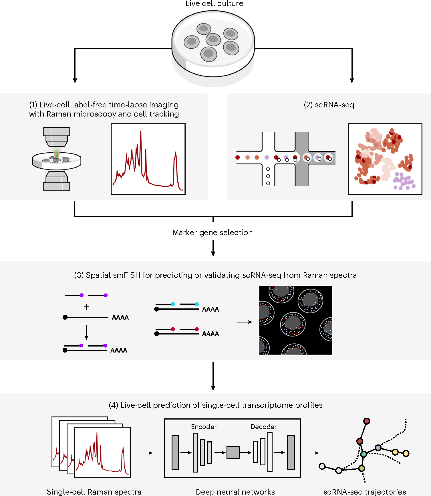
Live cells were cultured on gelatin-coated quartz glass-bottom plates (top) and Raman spectra were then measured at each pixel (at subcellular spatial resolution) within an image frame, and after time-lapse imaging and cell tracking (1), smFISH imaging in the same area was carried out (3). In an independent experiment, cells in the same system were dissociated into a single-cell suspension and profiled by scRNA-seq (2). scRNA-seq profiles were used to select nine marker genes for five major cell clusters for mouse iPS cell reprogramming and four marker genes for three major cell lineages in mES cell differentiation, and those were measured with spatial smFISH (3). Lastly, single-cell expression profiles were generated from Raman spectra of individual cells, by either anchor-based (measured by smFISH) or anchor-free methods (4) using fully connected neural networks and AAEs, respectively. Marker gene profiles measured by smFISH are used for either training or validation.

To facilitate data acquisition, we developed a high-throughput multimodal Raman microscope that enables the automated acquisition of Raman spectra, brightfield and fluorescent images. To this end, we integrated Raman microscopy optics to a fluorescence microscope, where high-speed galvo mirrors and motorized stages were combined to achieve scanning of a large field of view (FOV), and where dedicated electronics and software automated measurements across multiple modalities (Extended Data Fig. 1, Supplementary Fig. 1 and Methods).

We first demonstrated that R2R can infer profiles of two distinct cell types: mouse induced pluripotent stem (iPS) cells expressing an endogenous Oct4–green fluorescent protein (GFP) reporter and mouse fibroblasts¹⁶. To this end, we mixed the cells in equal proportions, plated them in a gelatin-coated quartz glass-bottom Petri dish, and performed live-cell Raman imaging, along with fluorescent imaging of a live-cell nucleus staining dye (Hoechst 33342) for cell segmentation and image registration, and an iPS cell marker gene, Oct4–GFP (Fig. 2a and Methods). The excitation wavelength for our Raman microscope (785 nm) was distant enough from the GFP Stokes shift emission, such that there was no interference with the cellular Raman spectra (Supplementary Fig. 2). Furthermore, there was no noticeable phototoxicity induced in the cells (Supplementary Fig. 3). After Raman and fluorescence imaging, we fixed and permeabilized the cells and performed smFISH of marker genes for mouse iPS cells (Nanog) and fibroblasts (Col1a1) with hybridization chain reaction (HCR¹⁷; Methods). We registered the nucleus stains, GFP images, HCR images and Raman images through either polystyrene control bead images or reference points marked under the glass-bottom dishes (Supplementary Fig. 4 and Methods).

Fig. 2 |. R2R accurately distinguishes cell types and predicts binary expression of marker genes in a mixture of mouse fibroblasts and iPS cells.

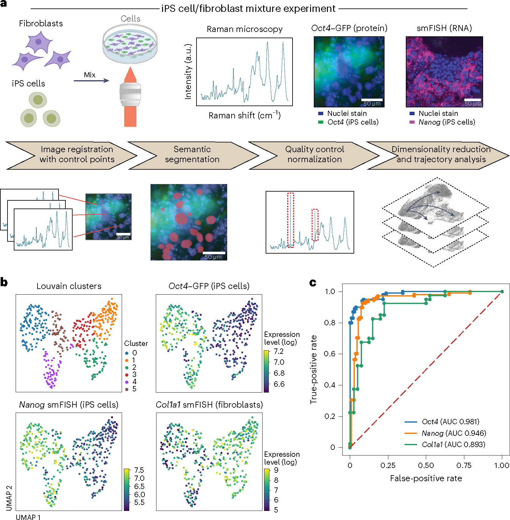
a, Overview. Top: experimental procedures. Mouse fibroblasts and iPS cells were mixed 1:1 and plated on glass-bottom plates, followed by Raman imaging of live cells, nucleus staining and measurement of endogenous Oct4–GFP (iPS cell marker) reporter by fluorescence imaging, and cell fixation and processing for smFISH with DAPI and probes for Nanog (iPS cells, magenta) and Col1a1 (fibroblasts). Bottom: preprocessing and analysis. From left: image registration with control points (Methods), followed by semantic cell segmentation, outlier removal/normalization and dimensionality reduction/trajectory analysis. b, R2R distinguishes cell states from Raman spectra. UMAP embedding of single-cell Raman spectra (dots) colored by Louvain clustering labels (top left) or smFISH measured expression of Oct4 (top right), Nanog (bottom left) and Col1a1 (bottom right). c, R2R accurately predicts binary (on/off) expression of marker genes. Receiver operating characteristic (ROC) plots and area under the curve (AUC) obtained by classifying the ‘on’ and ‘off’ states of Oct4 (blue), Nanog (orange) and Col1a1 (green).

The Raman spectra distinguished the two cell populations in a manner congruent with the expression of their respective reporters (measured live or by smFISH in the same cells), as reflected by a low-dimensional embedding of hyperspectral Raman data (Fig. 2b). Specifically, we focused on the fingerprint region of Raman spectra (600–1,800 cm⁻¹, capturing 930 of the 1,340 features in a Raman spectrum), where most of the signatures from various key biomolecules, such as proteins, nucleic acids and metabolites, lie¹¹. After basic preprocessing, including cosmic-ray and background removal and normalization, we aggregated Raman spectra that are confined to the nucleus, obtaining a 930-dimensional Raman spectroscopic representation for each cell’s nucleus. We then visualized these Raman profiles in an embedding in two dimensions using uniform manifold approximation and projection (UMAP)¹⁸ and labeled cells with the gene expression levels that were concurrently measured by either an Oct4–GFP reporter or smFISH (Fig. 2b). The cells separated clearly in their Raman profiles in a manner consistent with their gene expression characteristics, forming two main subsets in the embedding, one with cells with high Oct4 and Nanog expression (iPS cell markers) and another with cells with relatively high Col1a1 expression (fibroblast marker), indicating that Raman spectra are consistent with cell-intrinsic expression differences (Fig. 2b).

We further successfully trained a classifier to classify the ‘on’ or ‘off’ expression states of Oct4, Nanog and Col1a1 in each cell on the basis of its Raman profile (Methods). We trained a logistic regression classifier with 50% of the data and held out 50% for testing. We predicted Oct4 and Nanog expression states with high accuracy on the held-out test data (area under the receiver operating characteristic curve (AUROC) 0.98 and 0.95, respectively; Fig. 2c), indicating that expression of iPS cell markers can be predicted confidently from Raman spectra of live, label-free cells. We also successfully classified the expression state of the fibroblast marker Col1a1, albeit with lower confidence (AUROC 0.87; Fig. 2c), which is consistent with the lower contrast in Col1a1 expression (Fig. 2b) between iPS cells (Oct4⁺ or Nanog⁺ cells) versus non-iPS cells, compared to Oct4 or Nanog. Most misclassifications occurred when the ground truth expression level was near the threshold of the classifier, showing that misclassifications were probably due to the uncertainty in the ground truth expression (Supplementary Fig. 5).

Next, we asked if the Raman images could predict entire expression profiles nondestructively at single-cell resolution. To this end, we aimed to generate single-cell expression profiles from Raman images by multimodal data integration and translation, using multiplex smFISH data to anchor between the Raman images and scRNA-seq profiles (Fig. 3a). As a test case, we focused on mouse iPS cell reprogramming, where we have previously generated ~250,000 scRNA-seq profiles at half-day intervals throughout an 18-day, 36-time-point time course of reprogramming³ (Methods). Using WOT³ we selected from the scRNA-seq profiles nine anchor genes that represent diverse cell types that emerge during reprogramming (iPS cells: Nanog, Utf1 and Epcam; mesenchymal–epithelial transition (MET) and neural: Nnat and Fabp7; epithelial: Krt7 and Peg10; stromal: Bgn and Col1a1; Methods). We performed live-cell Raman imaging from day 8 of reprogramming, in which distinct cell types begin to emerge³, up to day 14.5, at half-day intervals, totaling 14 time points (Methods). We imaged ~500 cells per plate at 1 μm spatial resolution. Finally, we fixed cells immediately after each Raman imaging time point, followed by smFISH on the nine anchor genes (Methods). Strikingly, a low-dimensional representation of the Raman profiles showed that they encoded similar temporal dynamics to those observed with scRNA-seq during reprogramming (Fig. 3b,c and Supplementary Fig. 6), indicating that they may qualitatively mirror scRNA-seq.

Fig. 3 |. R2R predicts single-cell RNA profiles during reprogramming of mouse fibroblasts to iPS cells.

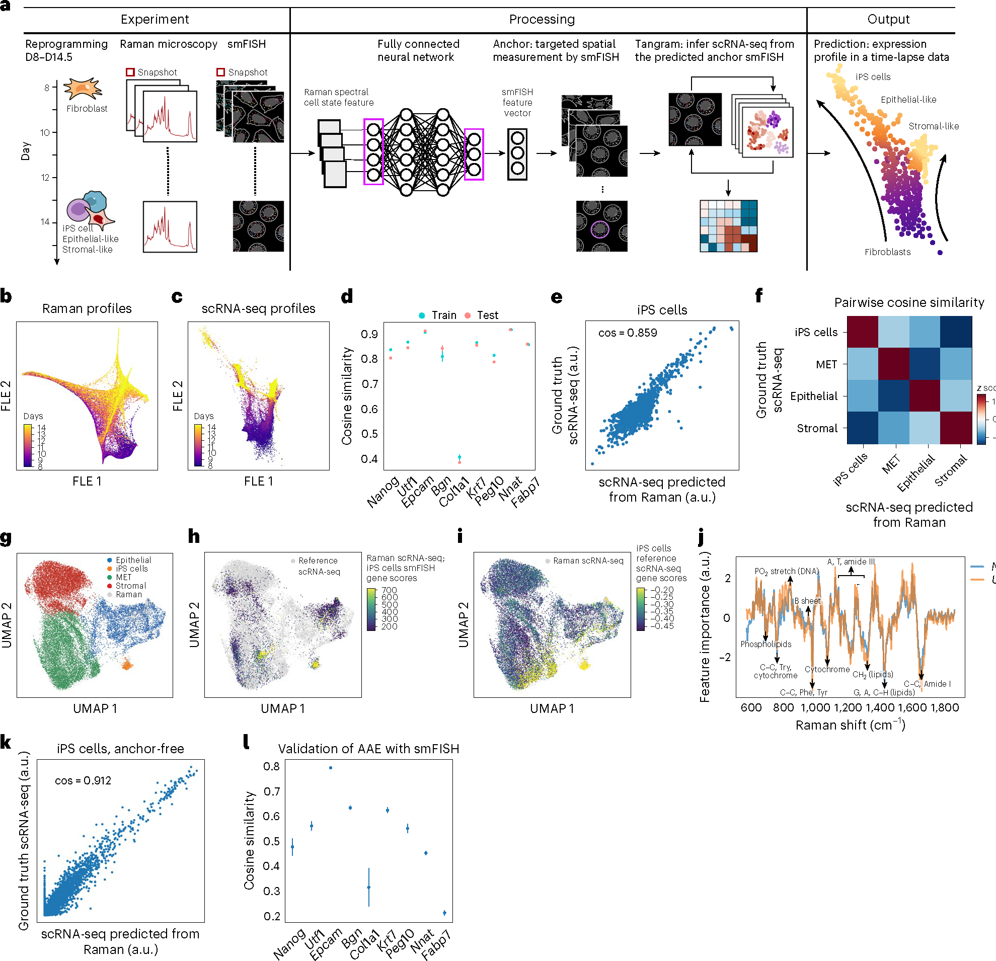
a, Anchor-based approach overview. From left: mouse fibroblasts were reprogrammed into iPS cells over the course of 14.5 days (‘D’), and, at half-day intervals from days 8 to 14.5, spatial Raman spectra, smFISH for nine anchor genes, and nucleus stains by fluorescence imaging were measured. Domain translation methods (fully connected neural network and Tangram) were used to predict scRNA-seq profiles from Raman spectra using smFISH as anchor. b,c, Low-dimensionality embedding by force-directed layout embedding (FLE) of Raman spectra (b, dots) or scRNA-seq (c, dots) profiles colored by measurement day (color bar). d, Cosine similarity (y axis) between measured (smFISH) and Raman-predicted levels for each smFISH anchor (x axis) in LOOCV where eight out of nine smFISH anchor genes were used for training, and the left-out gene was predicted. Error bars: standard error of five trials with different subset of cells, and mean value at center. e, Measured (y axis) and R2R-generated (x axis) pseudo-bulk RNA profiles (Supplementary Fig. 7) averaged across iPS cells of test cells for each of the top 2,000 highly variable genes (HVGs; dots). f, Pairwise cosine similarity (color bar, z score) between R2R-generated and scRNA-seq measured pseudo-bulk profiles (top 2,000 HVGs) in each cell type (rows, columns). g–i, UMAP co-embedding of R2R-generated RNA profiles on Raman test cells (not used for training) and measured scRNA-seq profiles (dots) colored by cell type annotations (g) or by iPS cell gene signature scores (Methods) of Raman-predicted profiles (h) or of real scRNA-seq (i). j, Feature importance scores of Raman spectra in predicting iPS cell-related marker genes (y axis) along the Raman spectrum (x axis). Known Raman peaks¹⁹ were annotated. k, Measured (y axis) and R2R-generated (x axis; anchor-free method) pseudo-bulk RNA profiles averaged across iPS cells for each of the top 2,000 HVGs (dots). l, Cosine similarity (y axis) between measured (smFISH) and anchor-free Raman-generated levels for each smFISH anchor (x axis). Error bars: standard error of five trials with different subset of cells, and mean value at center.

We next inferred scRNA-seq expression profiles from Raman images in two steps using the smFISH marker genes as anchors (Methods), first learning a fully connected neural net that predicts smFISH anchors from the Raman profiles (Methods) and then using Tangram¹⁵ to map from the predicted anchors to full scRNA-seq profiles (Figs. 1 and 3a). In the first step, we averaged the smFISH signal within a nucleus, yielding a nine-dimensional smFISH profile for each single nucleus. Then, we trained a deep neural net to translate Raman profiles to these nine-dimensional profiles using 50% of the paired Raman and smFISH profiles as training data. In the second step, we mapped the anchor smFISH profiles to full scRNA-seq using Tangram.

The anchor-based R2R yielded well-predicted single-cell RNA profiles, by several lines of evidence (Fig. 3d–f). First, we performed leave-one-out cross-validation (LOOCV), in which we used eight of the nine anchor genes to integrate Raman with scRNA-seq profiles and compared the predicted expression of the remaining gene to its smFISH measurements. There was a significant correlation between the predicted and measured smFISH expression for any left-out gene, albeit with lower performance for Col1a1 (as also noted above) (cosine similarity r ≈ 0.8 except Col1a1, P value <10⁻¹⁰⁰; Fig. 3d). Second, we compared the real (scRNA-seq measured) and R2R-generated expression profiles averaged across cells of the same cell type (‘pseudo-bulk’ for each of iPS cells, epithelial cells, stromal cells and MET). To this end, we first obtained the ‘ground truth’ cell types of R2R profiles by transferring scRNA-seq annotations to the paired real smFISH profiles in the test set using Tangram’s label transfer function, and based on the labels, averaged R2R’s generated profiles across the cells of a single cell type (Supplementary Fig. 7). The R2R-generated and scRNA-seq pseudo-bulk profiles per cell type were highly correlated (cosine similarity >0.85) (Fig. 3e,f and Extended Data Fig. 2), demonstrating the accuracy of R2R at the cell type level. Moreover, the R2R generated profiles could be correctly classified to their day label at half-day resolution and were reasonably correlated (in pseudo-bulk) to real profiles at each time point for each cell type at both the global profile and individual gene level (Supplementary Fig. 8), showing that the generated profiles can distinguish temporal changes during iPS cell reprograming. Consistently, projecting the R2R generated profiles of each cell onto an embedding learned from the real scRNA-seq shows that the generated profiles span the key cell types as captured in real profiles (Fig. 3g–i and Extended Data Figs. 3–7). We note that the predicted profiles had lower variance compared to real scRNA-seq. As this is observed even when only using smFISH profiles to infer scRNA-seq profiles (with no Raman data; Supplementary Fig. 9, right), we believe it mostly reflects the limited number and domain maladaptation of the smFISH anchor genes used for integration. To test the robustness of the predictions, we downsampled the number of cells and anchor genes used for training, finding that ~600 cells (approximately tenfold less than the original input) and four to five smFISH genes, were typically sufficient for reliable transcriptome generation as long as they covered the relevant cell types (Supplementary Figs. 10a,b and 11). Finally, we examind the ability to predict profiles at time points that were not used at training, finding that approximately time points suffice to predict correct profiles at other (withheld) time points for each subset, as long as the key branching points are covered (Supplementary Fig. 10c). Thus, a user may be able to consider a design where destructive training data are only collected at a few choice time points and the rest are predicted solely by the trained model.

Importantly, an analogous neural net model to either infer smFISH profiles or classify cell types from the corresponding brightfield images (Supplementary Fig. 12 and Methods) had poor performance for predicting each of the nine smFISH genes in LOOCV (cosine similarity <0.15) and poor classification accuracy (F-scores iPS cells: 26.6%, epithelial: 27.9%, MET: 46.3%, stromal: 1.1%) (Supplementary Fig. 13). This suggests that brightfield z-stack images, unlike Raman spectra, either do not have the necessary information to infer expression profiles or require substantial modifications in the neural network architecture.

Specific Raman spectral features were correlated with expression levels based on their feature importance scores in R2R predictions (Methods, Fig. 3j and Extended Data Fig. 8). For example, Raman bands at approximately 752 cm⁻¹ (C–C, Try, cytochrome), 1,004 cm⁻¹ (CC, Phe, Tyr) and 1,445 cm⁻¹ (G, A, C–H, lipids) contributed to predicting iPS cell-related expression profiles, which is consistent with previous research that employed single-cell Raman spectra to identify mouse (m)ES cells¹⁹. The contributions of these bands were either suppressed or increased for other cell types, such as stromal or epithelial cells (Extended Data Fig. 8). These results highlight R2R as a unique method to relate Raman spectroscopic profiles, which reflect on various molecules such as metabolites and proteins, to expression profiles at the single-cell level.

Because spatial gene expression measurements (for example, by smFISH or spatial transcriptomics) are typically not paired with Raman measurements of the same cells, and anchor gene integration may cause domain maladaptation (Supplementary Fig. 9), we explored whether we can perform a ‘one-step’, anchor-free translation using an AAE. With the underlying assumption that both Raman and scRNA-seq arise from a common latent space, we trained an AAE with unpaired measurements of Raman and scRNA-seq, while simultaneously adversarially training a classifier that aims to tell apart a Raman from a scRNA-seq profile. The training continued until the classifier could not distinguish the two modalities in their low-dimensional embeddings, that is, the two were aligned in a common latent space (Methods and Extended Data Fig. 9). We trained our AAEs using 50% of the Raman profiles as training data and the remaining 50% as test data, to which we applied the trained AAE to generate anchor-free scRNA-seq profiles. For evaluation, the real smFISH of test cells was used by Tangram’s label transfer function to transfer labels of annotated scRNA-seq profiles to the measured (ground truth) smFISH profiles in the test set. Because using only unpaired Raman and scRNA-seq profiles in the training did not succeed in our hand, we loosely guided the AAE training with the training cells’ ground-truth cell type labels (which were determined by smFISH; Methods). We then used the trained AAE for anchor-free generation of accurate profiles (cosine similarity >0.9) (Fig. 3k,l, Extended Data Fig. 10 and Supplementary Fig. 14), albeit with decreased cell type classification accuracy compared to anchor-based generation (~26% decrease in pairwise correlation z score; compare Fig. 3d and Fig. 3l). The better classification accuracy of an anchor-based model is expected, but comes at a cost. The anchor-free approach resulted in predicted profiles with better overall correlation and more characteristic variance to real profiles, suggesting improved domain adaptation (Fig. 3e versus Fig. 3k and Supplementary Fig. 9 versus Extended Data Fig. 10). Moreover, because the anchor-free method requires only the ground truth of cell types, one can probably substitute smFISH with live-cell compatible dyes, fluorescent markers or cell surface protein markers, alleviating the need for destructive smFISH profiles. Overall, anchor-free generation shows promise for adding Raman microscopy to systems already profiled by scRNA-seq without the need to transfer through spatial expression anchors.

To illustrate the power of R2R to track live cells and study their dynamics in a genomically interpretable way, we performed R2R in live-cell time-lapse measurements during the differentiation of mES cells treated with retinoic acid (RA)²⁰ (Fig. 4a). Under RA treatment, mES cells differentiate into epiblast, ectoderm or extraembryonic endoderm (XEN)-like cells over 48–72 h (ref. 20). We first took Raman snapshot measurements across time points (seven time points at ~12-h intervals, one plate per time point), followed by smFISH on four lineage-specific anchor genes (ES cells: Pou5f1, epiblasts: Dppa2, ectoderm: Hoxb2, XEN: Sox17)²⁰. In parallel, on a separate plate, we conducted Raman time-lapse measurements to track the differentiation process over time (Fig. 4a and Methods). Using ~3,500 previously published scRNA-seq profiles²⁰, generated at either half- or 1-day intervals across a 4-day time course, we co-embedded real and R2R-generated (anchor-based, from snapshot data) single-cell expression profiles, finding good agreement (Fig. 4b–f and Supplementary Fig. 15). The R2R-generated profiles predicted the four smFISH genes (Fig. 4e,f,k and Supplementary Fig. 16) and cell type-specific pseudo-bulk profiles²⁰ (Fig. 4g,h) with reasonable accuracy. Morevover, the cell type-specific differentially expressed genes of R2R-generated profiles were similarly enriched²¹ for functional gene sets as the original profiles (Supplementary Fig. 17). These included ‘mechanisms associated with pluripotency’ in ES cells and epiblasts, ‘negative regulation of differentiation’ in ES cells, ‘epithelial differentiation’ in ectoderm and ‘collagen formation’ in XEN. Thus, R2R-generated profiles capture correct biological processes.

Fig. 4 |. R2R tracks and predicts gene expression dynamics in live single cells during mES cell differentiation.

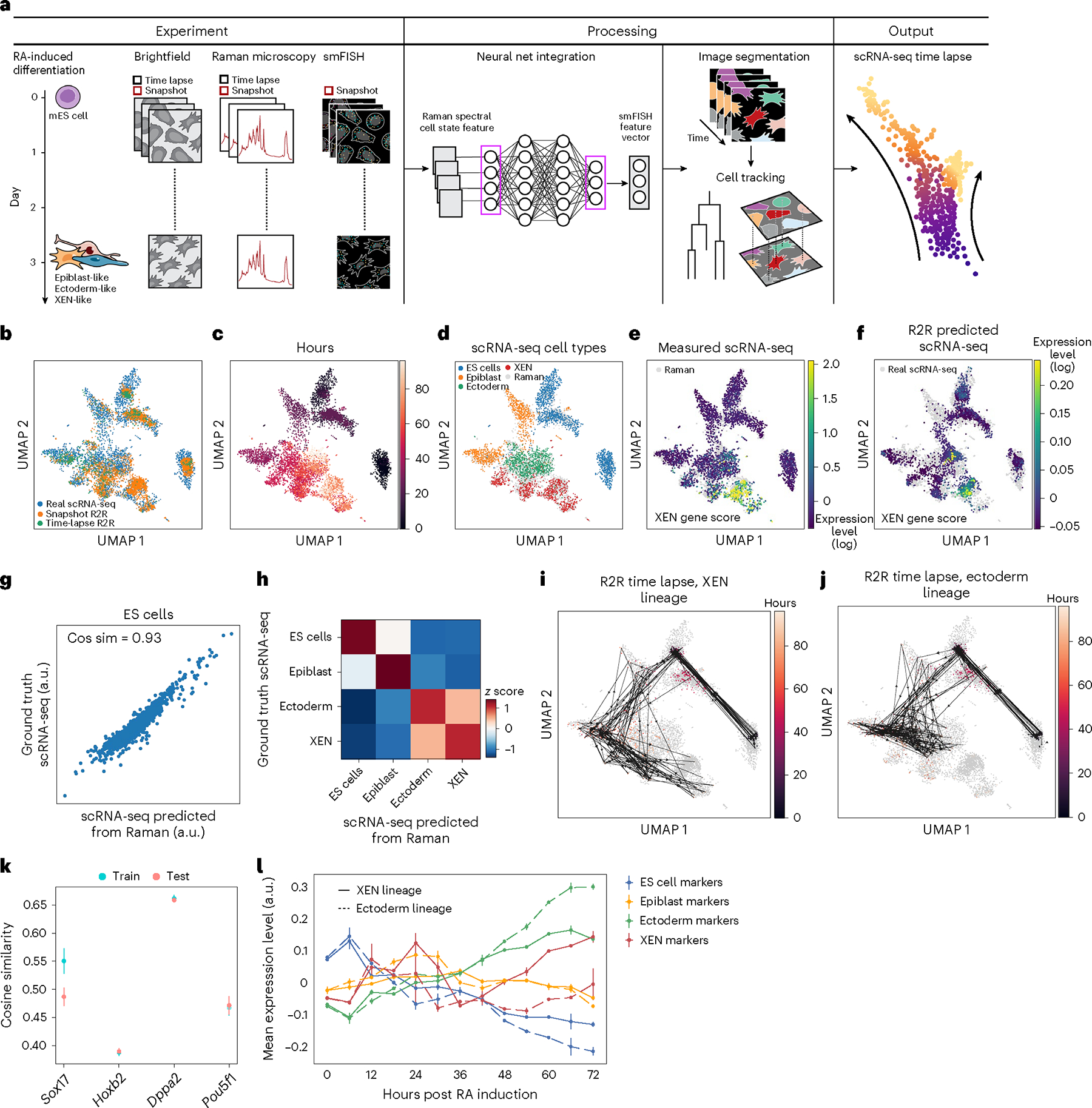
a, Overview. Snapshot Raman, smFISH and brightfield images were obtained every 12 h, and time-lapse Raman and brightfield were collected every 6 h and 30 min, respectively. scRNA-seq was collected in an independent experiment²⁰. Anchor-based R2R was trained on the paired Raman and smFISH data and applied to generate scRNA-seq from the Raman time-lapse data. b–f, Anchor-based R2R generates cell profiles consistent with a scRNA-seq time course. UMAP co-embedding of R2R-generated and measured (scRNA-seq) profiles (dots) colored by source of cell (b), time point (c), scRNA-seq cell types (d), scRNA-seq measured gene score of XEN marker gene²⁰ expression (e), or R2R-predicted gene score of XEN marker gene expression (f). g, scRNA-seq measured (y axis) and R2R-predicted (x axis) for each gene (dot) in pseudo-bulk RNA profiles averaged across mES cells at day 0. h, Pairwise correlation (color bar) between anchor-free Raman-predicted and scRNA-seq measured pseudo-bulk profiles in each cell type (rows, columns). i,j, Live cell tracking layered on R2R-generated profiles. UMAP as in c but with R2R-generated profiles connected by live cell tracking of underlying cells from brightfield time-lapse images that lead either to XEN-like (i) or ectoderm-like (j) cell fate. k, Prediction of smFISH anchors from Raman spectra. Cosine similarity (y axis) between measured (smFISH) and Raman-predicted levels for each smFISH anchor (x axis) in LOOCV, where three out of four smFISH anchor genes were used for training, and the left-out gene was predicted. Error bars: standard error of five trials with different subset of cells, and mean values at center. l, Mean expression (y axis) of marker genes (color) of each lineage (color) at different time points (x axis) post RA induction along XEN-like (solid) and ectoderm-like (dashed) trajectories. Error bars: standard error of expression level across cells with same lineage (n_ectoderm = 148, n_XEN = 200).

Next, we applied the trained R2R model to our Raman time-lapse measurements, yielding transcriptome information of direct cell lineages through live cell tracking (Methods), a unique feature of R2R. Once inferred, we could both track the inferred measurement of expression of a gene of interest over time in individual cells (Supplementary Fig. 18b), and layer live tracking over comprehensive Raman-generated expression profiles (Fig. 4i,j and Supplementary Fig. 18a). In this way, we observe that the differentiation of mES cells into epiblasts occurs around 24 hours, followed by ectoderm-like or XEN-like cells (Fig. 4i,j). Notably, R2R detected ectoderm versus XEN lineage divergence from as early as 48 h (Fig. 4l), a time point not easily tracked in scRNA-seq-based studies²⁰. The early lineage divergence in response to RA treatment is most probably associated with the activation of ectoderm- and XEN-like gene programs, which are distinguishable through the ground truth of time-lapse measurements but not by scRNA-seq at that time point, and yet are known to be validated by literature²⁰. Importantly, state-of-the-art computational methods, such as the pseudo-time algorithm and RNA velocity method in CellRank²², applied with default parameters to the real scRNA-seq data produced nonsensical results in this context, such as epiblasts ‘reprogramming’ back to mES cells (Supplementary Fig. 18c,d). Similar cases have been reported where different variations of RNA velocity yield contradicting trajectories from the same data^5,7,22,23. Even WOT³, which incorporates time point information for each cell explicitly (Supplementary Fig. 18e), did not reveal lineage differences as early or effectively as R2R, nor can it do so deterministically. In summary, this shows the broad and unique application of R2R for understanding the molecular dynamics in live cells.

Finally, we examined the specificity versus generalizability of the learned R2R models across biological systems, hypothesizing that in this current setting the model needs to be trained for each system. To this end, we used the anchor-free model trained on the iPS cell reprogramming system to generate scRNA-seq profiles from Raman measurements from the mES cell differentiation system, and compared the generated profiles to measured scRNA-seq profiles. As expected, both pseudo-bulk and pairwise comparisons of the profiles showed decreased accuracy for each cell type, with better performance for cells with similarities between the systems, such as mES cells (cosine similarity 0.533) and epiblasts (0.432), and very poor performance for cell types that are completely distinct (ectoderm 0.093, endoderm −0.194) (Supplementary Fig. 19). This results suggest that, while there is some transferable information, a more foundational R2R model that can generalize would require training on a greater variety of biological systems.

In conclusion, we reported R2R, a label-free nondestructive framework for inferring single-cell expression profiles from Raman spectra of live cells. Our framework conceptually differs from approaches that gauge specific Raman spectral bands to specific molecules^24,25, but rather aims to associate cell states defined by spectral bands to those defined by RNA profiles. We integrated Raman hyperspectral images with scRNA-seq data through paired or unpaired RNA and Raman measurements with multimodal data integration by Tangram or AAEs, respectively, and inferred single-cell expression profiles with high accuracy based on both averages within cell types and co-embeddings of individual profiles. We further showed that predictions using brightfield z-stacks had poor performance, indicating the importance of hyperspectral Raman microscopy for predicting expression profiles. Lastly, we applied R2R in live-cell time-lapse measurements, and demonstrated that expression profiles of the same live cell can be inferred over time, which is critical in settings where trajectory inference methods fail to reconstruct correct biological relations. To facilitate such applications, we provide a ‘How To’ guide (Supplementary Note) to construct a similar setup and release all the associate code we developed to operate the microscope.

R2R can be further developed in several ways. First, the throughput of single-cell Raman microscopy is still limited. In this pilot study, we profiled ~10,000 cells in each system. By using emerging vibrational spectroscopy techniques, such as stimulated Raman scattering microscopy²⁶ or photothermal microscopy^27,28, we envision increasing throughput by several orders of magnitude, to match the throughput of massively parallel single-cell genomics. Second, because molecular circuits and gene regulation are structured, with strong co-variation in gene expression profiles across cells, we can leverage the advances in computational microscopy to infer high-resolution data from low-resolution data, such as by using compressed sensing, to further increase throughput²⁹. Third, increasing the number of anchor genes (for example, by seqFISH³⁰, merFISH³¹, STARmap³² or ExSeq³³) can increase our prediction accuracy and capture more single-cell variance; our current results suggest that R2R may best predict the expression of highly variable genes. Fourth, using cell membrane dyes (combined with confocal fluorescent microscopes) or cytosol Raman bands could help with distinguishing nuclear from cytoplasmic states, and match with nuclear or cytoplasmic RNA profiling^34,35. Fifth, the adversarial networks that we used for unpaired training were relatively unstable, and other domain translation architectures, such as contrastive learning³⁶, may be able to produce more stable results. Finally, with single-cell multi-omics, we can project other modalities, such as scATAC-seq, to better capture the comprehensive nature of Raman spectra and explore the relation across different modalities. Moreover, generating training data across diverse cell systems at the cellular level—and in the future the organism level—may allow training more foundational models that generalize across biological systems and conditions. Overall, with further advances in single-cell genomics, imaging and machine learning, R2R could allow us to nondestructively investigate genome-wide molecular dynamics and complex biological processes through inferred profiles at scale in vitro, and possibly in vivo in living organisms.

Online content

Any methods, additional references, Nature Portfolio reporting summaries, source data, extended data, supplementary information, acknowledgements, peer review information; details of author contributions and competing interests; and statements of data and code availability are available at https://doi.org/10.1038/s41587-023-02082-2.

Methods

Mouse fibroblast reprogramming

OKSM secondary mouse embryonic fibroblasts (MEFs) were derived from E13.5 female embryos with a mixed B6;129 background. The cell line used in this study was homozygous for ROSA26-M2rtTA, homozygous for a polycistronic cassette carrying Oct4, Klf4, Sox2 and Myc at the Col1a1 3′ end, and homozygous for an EGFP reporter under the control of the Oct4 promoter. Briefly, MEFs were isolated from E13.5 embryos from timed matings by removing the head, limbs and internal organs under a dissecting microscope. The remaining tissue was finely minced using scalpels and dissociated by incubation at 37 °C for 10 min in trypsin–ethylenediaminetetraacetic acid (ThermoFisher Scientific). Dissociated cells were then plated in MEF medium containing Dulbecco’s modified Eagle medium (DMEM; ThermoFisher Scientific), supplemented with 10% fetal bovine serum (GE Healthcare Life Sciences), nonessential amino acids (ThermoFisher Scientific) and GlutaMAX (ThermoFisher Scientific). MEFs were cultured at 37 °C and 4% CO₂ and passaged until confluent. All procedures, including maintenance of animals, were performed according to a mouse protocol (2006N000104) approved by the MGH Subcommittee on Research Animal Care³.

For the reprogramming assay, 50,000 low-passage MEFs (no more than three to four passages from isolation) were seeded in 14 3.5-cm quartz glass-bottom Petri dishes (Waken B Tech) coated with gelatin. These cells were cultured at 37 °C and 5% CO₂ in reprogramming medium containing KnockOut DMEM (Gibco), 10% knockout serum replacement (Gibco), 10% fetal bovine serum (Gibco), 1% GlutaMAX (Invitrogen), 1% nonessential amino acids (Invitrogen), 0.055 mM 2-mercaptoethanol (Sigma), 1% penicillin–streptomycin (Invitrogen) and 1,000 U ml⁻¹ leukemia inhibitory factor (LIF, Millipore). Day 0 medium was supplemented with 2 mg ml⁻¹ doxycycline Phase-1 (Dox) to induce the polycistronic OKSM expression cassette. The medium was refreshed every other day. On day 8, doxycycline was withdrawn. Fresh medium was added every other day until the final time point on day 14. One plate was taken every 0.5 days after day 8 (D8 to D14.5) for Raman imaging and fixed with 4% formaldehyde immediately after for HCR.

High-throughput multimodal Raman microscope and time-lapse imaging

We developed an automated high-throughput multimodal microscope capable of multi-position and multi-time-point fluorescence imaging and point scanning Raman microscopy (Extended Data Fig. 1). A 749-nm short-pass filter was placed to separate brightfield and fluorescence from Raman scattering signal, and the fluorescence and Raman imaging modes were switched by swapping dichroic filters with auto-turrets. To realize a high-throughput Raman measurement, galvo mirror-based point scanning and stage scanning was combined to acquire each FOV and multiple different FOVs, respectively.

To realize this in an automated fashion, a MATLAB (2020b) script that communicates with Micro-manager³⁷, a digital acquisition board, and Raman scattering detector (Princeton Instruments, PIXIS 100BR eXcelon) was written (Extended Data Fig. 2). A 2D point scan Raman imaging sequence was regarded as a dummy image acquisition in Micro-manager, during which the script communicated via the digital acquisition board with (1) the detector to read out a spectrum, (2) the mirror to update the mirror angles and (3) shutters to control laser exposure. All communications were realized using transistor–transistor logic signaling. Updating of the galvo mirror angles was conducted during the readout of the detector. While the script ran in the background, Micro-manager initiated a multidimensional acquisition consisting of brightfield, 4′,6-diamidino-2-phenylindole (DAPI), GFP and dummy Raman channel at multiple positions and z-stacks.

An Olympus IX83 fluorescence microscope body was integrated with a 785-nm Raman excitation laser coupled to the backport, where the short-pass filter deflected the excitation to the sample through an Olympus UPLSAPO 60× numerical aperture 1.2 water immersion objective. The backscattered light was collimated through the same objective and collected with a 50-μm core multimode fiber, which was then sent to the spectrograph (Holospec f/1.8i 785 nm model) and detector. The fluorescence and brightfield channels were imaged by the Orca Flash 4.0 v2 sCMOS camera from Hamamatsu Photonics. The exposure time for each point in the Raman measurement was 20 ms, readout time of the detector was 16 ms, and laser power at the sample plane was 212 mW. Each FOV was 100 × 100 pixels, with each pixel corresponding to about 1 μm. The laser source was a 785-nm Ti-Sapphire laser cavity coupled to a 532-nm pump laser operating at 4.7 W.

The time to acquire Raman hyperspectral images was roughly 8 min per FOV. With 8 min, it is unrealistic to image an entire glass-bottom plate. Therefore, for the iPS cell reprogramming system, representative FOVs that cover all representative cell types were chosen by visual inspection, including iPS cell-like, epithelial-like, stromal-like and MET cells. Twenty-one FOVs were chosen for each plate, where roughly 15 FOVs were from the boundaries of colonies, 5 from noncolonies and 1 from noncells to use for background correction in reprogramming cells. For mES cell differentiation, 20 FOVs were chosen that cover mES cells, epiblast-like, ectoderm-like and XEN-like cells and 1 FOV for background correction.

Due to the extended Raman imaging time, evaporation of the immersion water was no longer negligible. Therefore, we developed an automated water immersion feeder using syringe pumps and syringe needles glued to the tip of the objective lens. Here, water was supplied at a flow rate of 1 μl min⁻¹.

For time-lapse measurements in mES cells, Raman measurements were carried out every 6 h, whereas for brightfield imaging it was every 30 min. Measurement were halted at 72 h, as after that time point, differentiation led to cell death, making cell tracking challenging.

iPS cell and MEF mixture experiment

Low-passage iPS cells were first cultured in N2B27 2i media containing 3 mM CHIR99021, 1 mM PD0325901 and LIF. On the day of the experiment, 750,000 iPS cells and 750,000 MEFs were plated on the same gelatin-coated 3.5-cm quartz glass-bottom Petri dish. Cells were plated in the same reprogramming medium as previously described (with Dox) with the exception of utilizing DMEM without phenol red (Gibco) instead of KnockOut DMEM. Six hours after plating, the quartz dishes were taken for Raman imaging and fixed with 4% formaldehyde immediately after for HCR.

mES cell differentiation experiment

For mES cell differentiation, we followed the protocol described by Semrau et al.²⁰. Briefly, 40,000 V6.5 mES cells were plated onto 35-mm quartz bottom plates with a 10% gelatin coating and grown overnight, using modified 2i medium plus LIF (2i/L) containing no phenol-red DMEM/F12 (Life Technologies) and supplemented with 0.5× N2 supplement (Gibco), 0.5× B27 supplement (Gibco), 0.5 mM L-glutamine (Gibco), 20 μg ml⁻¹ human insulin (Sigma-Aldrich), 1× 100 U ml⁻¹ penicillin/streptomycin (Gibco), 0.5× MEM nonessential amino acids (Gibco), 0.1 mM 2-mercaptoethanol (Sigma-Aldrich), 1 μM MEK inhibitor (PD0325901, Stemgent), 3 μM GSK3 inhibitor (CHIR99021, Stemgent) and 1,000 U ml⁻¹ mouse LIF (ESGRO). The next day, cells were washed twice with phosphate-buffered saline and differentiation medium was added. The differentiation medium used was basal N2B27 medium (2i/L without the inhibitors, LIF, and insulin) supplemented with all-trans RA (Sigma-Aldrich) at 0.25 μM unless stated otherwise. Spent medium was exchanged with fresh medium every 48 h.

Anchor gene selection by WOT

To select anchor genes for connecting spatial information to the full transcriptome data, WOT³ was applied to mouse fibroblast reprogramming scRNA-seq data collected at matching time points and culture condition (days 8 to 14.5 at half-day intervals)³. For each cell fate, the transition probabilities of each cell toward iPS cells, epithelial-like or stromal-like cells were calculated and the cells with the top 10 percentile transition probabilities were selected per time point (Extended Data Fig. 6). Next, the FindMarker function in Seurat³⁸ was used to find genes differentially expressed in these cell subsets versus all other cells per time point. Through this approach, two genes were chosen per cell type that are both found by Seurat and commonly used for these cell types (iPS cells: Nanog, Utf1; epithelial: Krt7, Peg10; stromal: Bgn, Col1a1; MET and neural: Fabp7, Nnat), along with Epcam, an established early marker of iPS cells and epithelial cells in this system^3,39.

smFISH by HCR

Fixed samples were prepared for imaging using the HCR v3.0 protocol for mammalian cells on a chambered slide, incubating at the amplification step for 45 min in the dark at room temperature. Three probes with amplifiers conjugated to fluorophores Alexa Fluor 488, Alexa Fluor 546 and Alexa Fluor 647 were used. Samples were stained with DAPI before imaging. After imaging, probes were stripped from samples by washing samples once for 5 minutes in 80% formamide at room temperature and then incubating three times for 30 min in 80% formamide at 37 °C. Samples were washed once more with 80% formamide, then once with phosphate-buffered saline, and reprobed with another panel of probes for subsequent imaging.

Image registration of Raman hyperspectral images and fluorescence/smFISH images

Brightfield and fluorescence channels including DAPI and GFP, along with corresponding Raman images, were registered by using 5-μm fluorescent polystyrene beads deposited on quartz glass-bottom Petri dishes (SF-S-D12, Waken B Tech) as calibration. The brightfield and fluorescence images of the beads were then registered by the scale-invariant template matching algorithm of the OpenCV⁴⁰ matchTemplate function followed by manual correction.

For the registration of smFISH and Raman images, four marks inscribed under the glass-bottom Petri dishes were used as reference points (Extended Data Fig. 4). As the Petri dishes are temporarily removed from the Raman microscope after imaging to do smFISH measurements, the dishes cannot be placed back at the same exact location on the microscope. Therefore, the coordinates of these reference points were measured along with the different FOVs. When the dishes were placed again after smFISH measurements, the reference mark coordinates were measured, and an affine mapping was constructed to calculate the new FOV coordinates. Lastly, as smFISH consisted of three rounds of hybridization and imaging, the following steps were performed to register images across different rounds with a custom MATLAB script:

1. Maximum intensity projection of nuclei stain and RNA images

2. Automatic registration of round 1 images to rounds 2 and 3 based on nuclei stain images and MATLAB function imregtform. First, initial registration transformation functions were obtained with a similarity transformation model passing the ‘multimodal’ configuration. Then, those transformations were used as the initial conditions for an affine model-based registration with the imregtform function. Finally, this affine mapping transformation was applied to all the smFISH (RNA) images.

3. Use the protocol in (2) to register nuclei stain images obtained from the multimodal Raman microscope and the first round of images used for smFISH. Then, apply the transformation to the remaining second and third rounds.

4. Manually remove registration outliers in (3). Approximately 10% of the images were removed.

Fibroblast cells were mobile during the two-class mixture experiment so that, by the time Raman imaging finished, cells had moved far enough from their original position that the above semi-automated strategy could not be applied. Thus, ~100 cells were manually identified as present in nuclei stain images both before and after Raman imaging.

Hyperspectral Raman image processing

Each raw Raman spectrum has 1,340 channels. Of those channels, we extracted the fingerprint region (600–1,800 cm⁻¹), which resulted in a total of 930 channels per spectrum. Thus, each FOV is a 100 × 100 × 930 hyperspectral image. As samples were scanned at 1-μm steps, the FOV corresponded to a 100-by-100 μm² region. The hyperspectral images were then preprocessed by a Python script as follows:

1. Cosmic ray removal. Cosmic rays were detected by subtracting the median filtered spectra from the raw spectra, and any feature above 5 was classified as an outlier and replaced with the median value. The kernel window size for the median filter was 7.

2. Autofluorescence removal. The baseline function in rampy⁴¹, a Python package for Raman spectral preprocessing, was used with the alternating least squares algorithm ‘als’.

3. Savitzky–Golay smoothing. The scipy.signal.savgol_filter function was used with window size 5 and polynomial order 3.

4. Averaging spectra at the single-cell level. Nuclei stain images were segmented using NucleAIzer⁴² and averaged pixel-level spectra that fall within each nucleus.

5. Spectra standardization. Spectra were standardized to a mean of 0 and a standard deviation of 1.

Anchored generation of scRNA-seq profiles from paired Raman spectra and smFISH

Anchored generation of scRNA-seq profiles consists of two steps: (1) prediction of anchor smFISH profiles from Raman profiles using a fully connected neural net, and (2) integration of predicted smFISH profile to scRNA-seq using Tangram¹⁵.

The neural network model to predict smFISH from Raman spectra consisted of three Linear, BatchNorm, ReLU activation blocks in sequence. Letting n be the number of input spectra, the number of nodes in these three blocks were, in order, n, 512, 128, 10. Input smFISH data were normalized, per gene, using min–max normalization before training. Training was carried out on an NVIDIA Tesla P100 graphics processing unit (GPU), according to a mean square error loss, for 100 epochs with a learning rate of 0.00001 on an Adam Optimizer and a batch size of 64.

The predicted smFISH was integrated with expression profiles using Tangram¹⁵, a method that aligns scRNA-seq profiles to spatial measurements of a small number of genes. Tangram’s map_cells_to_space function was applied (learning_rate 0.1, num_epochs 1000) on an NVIDIA Tesla P100 GPU, followed by Tangram’s project_genes function.

To assess performance, 50% of the paired smFISH-Raman data were used for training and the remaining 50% were held as test data (not validation data), as follows. The training Raman/smFISH partition was used to learn a Raman to smFISH neural net model. Then, the trained neural net model was applied to the Raman profiles in the test set to generate predicted smFISH data, and Tangram’s functions were used to generate predicted scRNA-seq profiles from the predicted smFISH. Separately, the real smFISH of test cells was used by Tangram’s label transfer function project_cell_annotations to transfer labels of annotated scRNA-seq profiles to the measured (ground truth) smFISH profiles in the test set. Finally, pseudo-bulk profiles were calculated per cell type for both R2R-predicted and real scRNA-seq and compared between them³ based on the cosine similarity, calculated as the dot product and magnitude of the predicted ($\mathbf{x}$) and ground truth ($\mathbf{y}$) measurements, $\mathrm{c}\mathrm{o}\mathrm{s}\mathrm{\theta }=\mathbf{x}\mathbf{y}/\Vert \mathbf{x}\Vert \Vert \mathbf{y}\Vert$.

For any classification tasks based on Raman spectra, a decision tree-based nonlinear regression Catboost⁴³ was used with the early stopping parameter set to 5.

Anchor-free generation of Raman and scRNA-seq profiles using AAEs

One-step anchor-free prediction was carried out with AAEs⁴⁴ consisting of three models: a gene-expression autoencoder, G, which reconstructed gene-expression data by encoding then decoding, a Raman-spectra autoencoder, R, similar to G but for Raman profiles, and an adversarial discriminator, A, which ensured that the encoders of G and R encoded to an identical latent domain. To accomplish this, first G was trained to reconstruct gene-expression data, after which R and A were trained ‘against’ each other, such that A was trained to differentiate between encodings by G and R, and R was trained such that, in addition to reconstructing Raman data, it was penalized when A correctly differentiated between encodings by G and by R. After training, to translate from Raman to gene expression, we encoded a Raman spectrum with R’s encoder and decoded a gene-expression profile with G’s decoder, made possible by the shared latent domain to which G and R encode.

However, the initial approach did not succeed in ensuring that cells of the same cell type in the Raman and gene-expression domains mapped to same parts of the latent space. We thus introduced an additional model, S, that classified latent encodings of G by cell type. S was trained after G but before R and A. When R was trained, in addition to being penalized when A correctly differentiated between encodings by G and by R, it was also penalized when the cell type of the cell’s encodings inferred by S was different from its assigned cell type. The ground truth cell types were given by the smFISH measurements for each Raman profile.

G, a deep neural network, consisted of 10 Linear, BatchNorm, ReLU activation blocks in sequence. Letting n be the number of input genes, 19,089, the number of nodes in these ten blocks were, in order, n, 2,048, 2,048, 2,048, 2,048, 512, 2,048, 2,048, 2,048, 2,048, n. R followed an architecture identical to G, but with n being 930, the number of Raman spectral features in each cell’s spectrum. A consisted of four Linear, Spectral Normalization, ReLU activation blocks. The numbers of nodes in each of these blocks are, in order, 128, 64, 32, 32, 2. S followed the same architecture as A, but with number of nodes in each of its blocks being, in order, 128, 64, 32, 32, 4.

G was trained according to a mean-square error loss function. S was then trained with a weighted cross-entropy loss function with one-hot vectors for cell types. R and A were then trained adversarially, taking turns between weight updates. A was trained according to a binary cross-entropy loss. S was also trained according to a binary cross-entropy loss. R was trained according to the following loss function:

$$f\left(\mathbf{r}\right)=\mathrm{M}\mathrm{S}\mathrm{E}(\mathbf{r},R(\mathbf{r}\left)\right)+{\lambda }_1\left(\mathrm{A}\mathrm{D}\mathrm{V}\right(A\left(R\right(\mathbf{r}\left)\right)\left)\right)+{\lambda }_2\left(\mathrm{C}\mathrm{E}\left(S\left(R\right(\mathbf{r}\left)\right),c_{\mathbf{r}}\right)\right)$$

where $\mathbf{r}$ was a Raman spectrum, ${\lambda }_1$ was $\mathbf{r}$’s cell type, ${\lambda }_2$ were regularizing constants, MSE($\mathbf{x},\mathbf{y}$) was a mean-square error loss between $\mathbf{x}$ and $\mathbf{y}$, ADV($\mathbf{x}$) was the cross-entropy loss against labels indicating $\mathbf{x}$ was a gene-expression encoding, and CE($\mathbf{x},\mathbf{y}$) was a cross-entropy loss between $\mathbf{x}$ and $\mathbf{y}$. All models were trained using the Adam optimizer, with Gs having a learning rate of 0.00001, Rs having 0.00005, As having 0.004 and Ss having 0.001. G was trained for 30 epochs, S was trained for 100 epochs, and R and A were trained together, adversarially, for 100 epochs. Training and inference was carried out by Pytorch 1.9.0 and Tensorflow 2.5.3.

To assess performance, 50% of the paired Raman/smFISH data were used for training and the remaining 50% were held as test data (not validation data). The training Raman/smFISH partition was used to learn a Raman to scRNA-seq AAE model along with the cell type information of the training cells (for which smFISH data were used). Here the cell types for training cells were given by Tangram’s label transfer function project_cell_annotations applied on the real smFISH of the training cells. Then, the trained neural net model was applied to the Raman profiles in the test set to generate predicted scRNA-seq profiles.

Separately, for evaluation of the predictions, the real smFISH data of test cells were used by Tangram’s label transfer function project_cell_annotations to transfer labels of annotated scRNA-seq profiles to the measured (ground truth) smFISH profiles in the test set. Finally, pseudo-bulk profiles were calculated per cell type for both R2R-predicted and real scRNA-seq³ and compared between them on the basis of the cosine similarity, calculated as the dot product and magnitude of the predicted ($\mathbf{x}$) and ground truth ($\mathbf{y}$) measurements, $\mathrm{c}\mathrm{o}\mathrm{s}\mathrm{\theta }=\mathbf{x}\mathbf{y}/\Vert \mathbf{x}\Vert \Vert \mathbf{y}\Vert$.

Inferring smFISH and cell types from brightfield images

To regress cellular smFISH levels from brightfield cell images, target cell masks were created where segmentation masks from nucleus stains were replaced with the average smFISH expression level, thereby averaging out any subcellular variations for a fair comparison with R2R predictions. A modified U-net with skip connections and residual blocks⁵ was trained to estimate the corresponding average smFISH per cell. Due to the small size of the available training set, data were augmented the rotation and flipping and a subsample 50 × 50 pixel region of each brightfield image was taken due to memory constraints. Training was carried out on an NVIDIA Tesla P100 GPU, with 100 epochs, a learning rate of 0.01 and a batch size of 400. For each smFISH prediction, the epoch with the validation score was selected.

For cell-type classification from brightfield images of individual cells, registered smFISH-brightfield images were broken into smaller 32-by-32 pixel nonoverlapping tiles and the average smFISH expression level was calculated for each tile (this tile size rougly corresponds to the size of one cell, but depending on the location and cell size can capture portions of more than one cell). Tangram was used with scRNA-seq data to map each tile’s average smFISH vector to a cell type. A convolutional neural network (CNN) was then trained to map a brightfield tile to a cell type. The CNN consisted of a convolutional layer with 11 input channels, 20 output channels, a kernel size of 5 and a stride of 1, followed by a ReLU activation layer, followed by a maximum-pool layer with a kernel size of 2 and a stride of 2, followed by another convolutional layer with 20 input channels, 20 output channels, a kernel size of 5 and a stride of 1, followed by another ReLU activation layer, followed by another maximum-pool layer with a kernel size of 2 and a stride of 2, followed by a reshaping layer to 500 nodes, another ReLU activation layer, and final fully connected layer to 4 final nodes. The CNN was trained via a cross-entropy loss with an Adam optimizer at a learning rate of 0.00003 for 20 epochs.

Dimensionality reduction, embedding and projection

For dimension reduction and visualization of Raman and scRNA-seq profiles, we performed forced layout embedding using the Pegasus pipeline⁴⁵. First, we performed principal component analysiś(PCA) on both Raman and scRNA-seq profiles independently, calculated diffusion maps on the top 100 principal components, and performed an approximated forced layout embedding graph using Deep Learning by pegasus.net_fle with default parameters.

To project Raman profiles to a scRNA-seq embedding, we calculated a k-nearest neighbor (k-NN) graph (k = 15) on the scRNA-seq top 50 principal components with the cosine metric, and UMAP with the scanpy.tl.umap function in Scanpy⁴⁶ version 1.7.2 with default parameters. Then, the Raman predicted expression profiles were projected on to the scRNA-seq UMAP embedding by scanpy.tl.ingest using k-NN as the labeling method and default parameters.

Feature importance analysis

To evaluate the contributions of Raman spectral features to expression profile prediction, we used the get_feature_importance function in Catboost. The early stopping parameter was set to 5. As the dimensions of Raman spectra were reduced by PCA before Catboost, feature importance scores were calculated for each principal component, and the weighted linear combination of the Raman PCA eigenvectors with feature scores as the weight was calculated to obtain the full spectrum.

Cell segmentation and tracking of Raman time-lapse images during mES cell differentiation

Nucleus stains such as DAPI or Hoechst 33342 require ultraviolet excitation, limiting long-term time-lapse imaging. Thus, cell segmentation of time-lapse measurements was performed by first converting brightfield z-stack images with f-net, a deep learning model that predicts fluorescent images from brightfield images⁴⁷. Here, ground truth nucleus stains of the corresponding brightfield images, obtained at snapshot time points, were used to train f-net, and the trained neural net was applied to real time-lapse images to produce ‘digital stains’. Then, Stardist⁴⁸ was applied to perform cell segmentation. Segmentation errors were manually corrected with Napari⁴⁹. Lastly, cell tracking was conducted by Bayesian Tracker⁵⁰.

Pseudo-time analysis was carried out by following the CellRank²² v1.3 pipeline. To calculate the transition matrix, the CytoTRACEKernel function was applied to mES cell scRNA-seq profiles²⁰, and then compute_transition_matrix was applied with default parameters to visualize the transition of cells across time.

For RNA velocity, first, mES cell scRNA-seq fastq reads⁵¹ were processed using zUMI⁵¹ v2.9.7. Splicing rates were quantified by velocyto⁴, and generalized RNA velocity was carried out by scVelo⁵ v0.2.5 using the dynamical model. In scVelo, tl.recover_dynamics was used to estimate velocity parameters, then tl.velocity with the ‘dynamical’ parameter to estimate velocity, and finally tl.velocity_graph was used to estimate the velocity graph.

Extended Data

Extended Data Fig. 1 |. A multi-modal Raman microscope capable of fluorescence imaging and Raman microscopy.

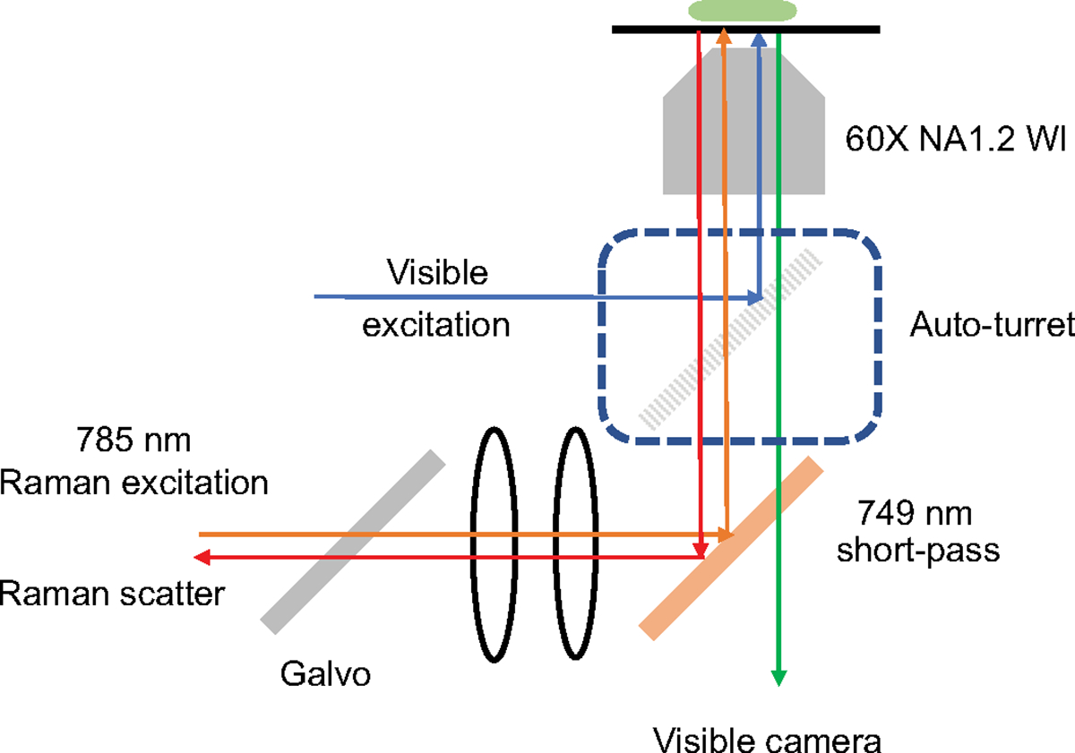
Schematic of a Raman microscope integrated with a wide-field fluorescence microscope for simultaneous detection of nuclei staining, bright field, fluorescence channels, and Raman images.

Extended Data Fig. 2 |. Raman-predicted and scRNA-seq measured pseudo-bulk profiles are well correlated across cell types.

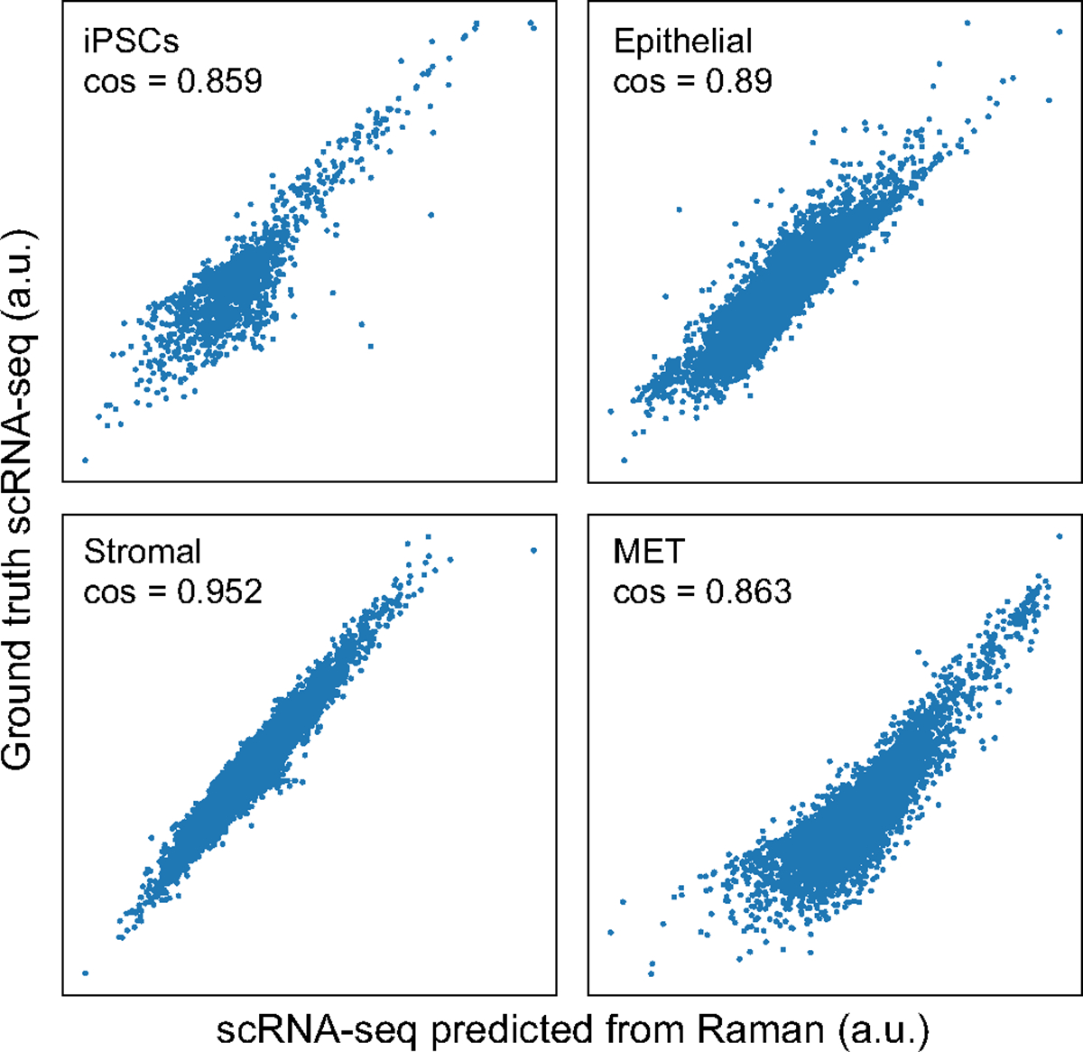
scRNA-seq measured (y axis) and R2R-predicted (x axis) expression for each gene (dot) in pseudo-bulk RNA profiles averaged across cells labeled as iPSC (top left), epithelial (top right), stromal (bottom left) and MET (bottom right). Cosine similarity is denoted at the top left corner.

Extended Data Fig. 3 |. Measured and Raman-predicted single cell profiles co-embed well as reflected by gene scores for each cell type.

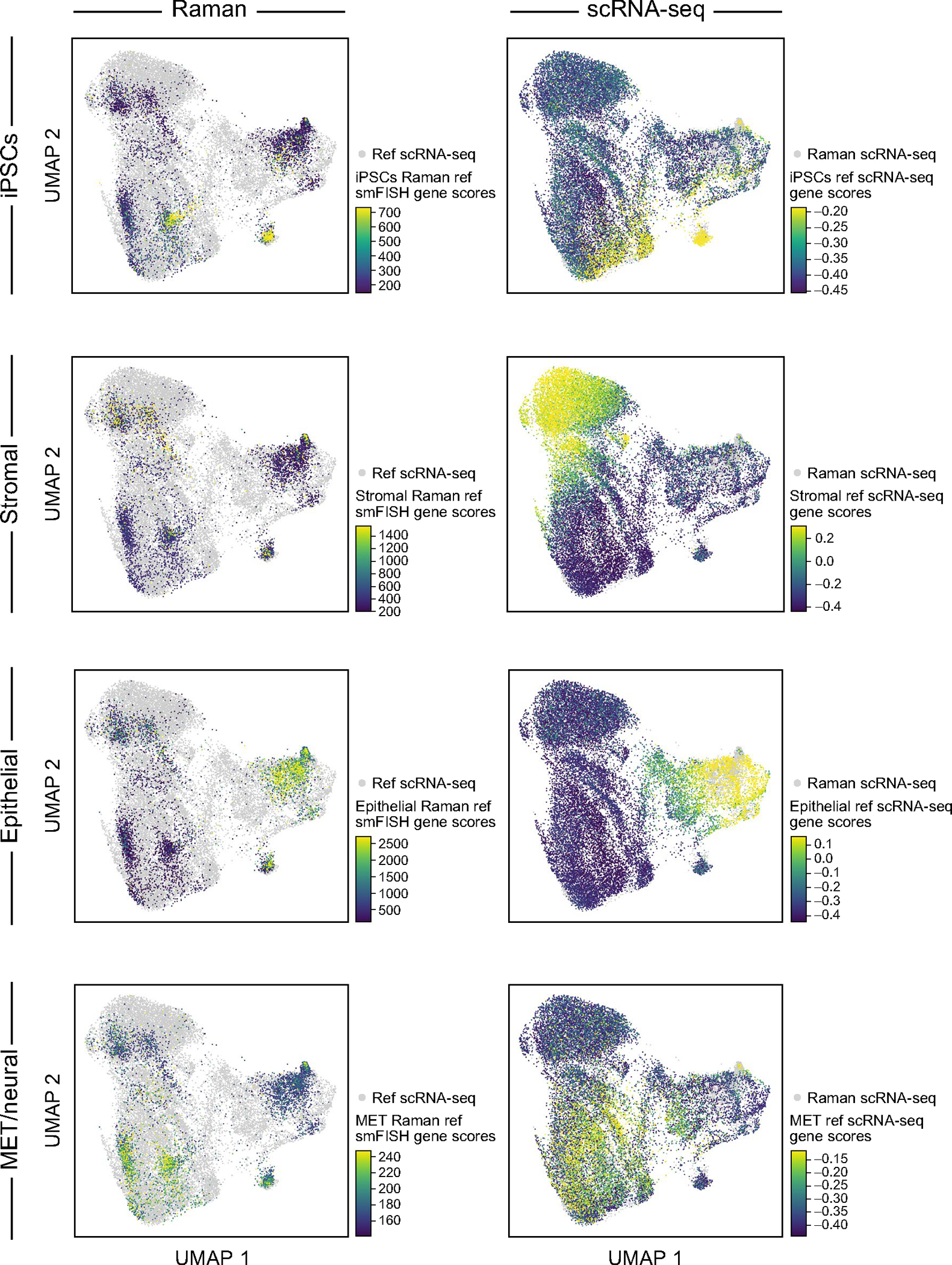
UMAP co-embedding of Raman predicted RNA profiles and measured scRNA-seq profiles (dots) colored by scores of marker gene for different cell types (rows) determined by smFISH measurements (left, for cells with Raman-predicted profiles) or real scRNA-seq measurements (right, for cells with scRNA-seq profiles).

Extended Data Fig. 4 |. Measured and Raman-predicted single cell profiles co-embed well as reflected by smFISH measurement of Raman cells.

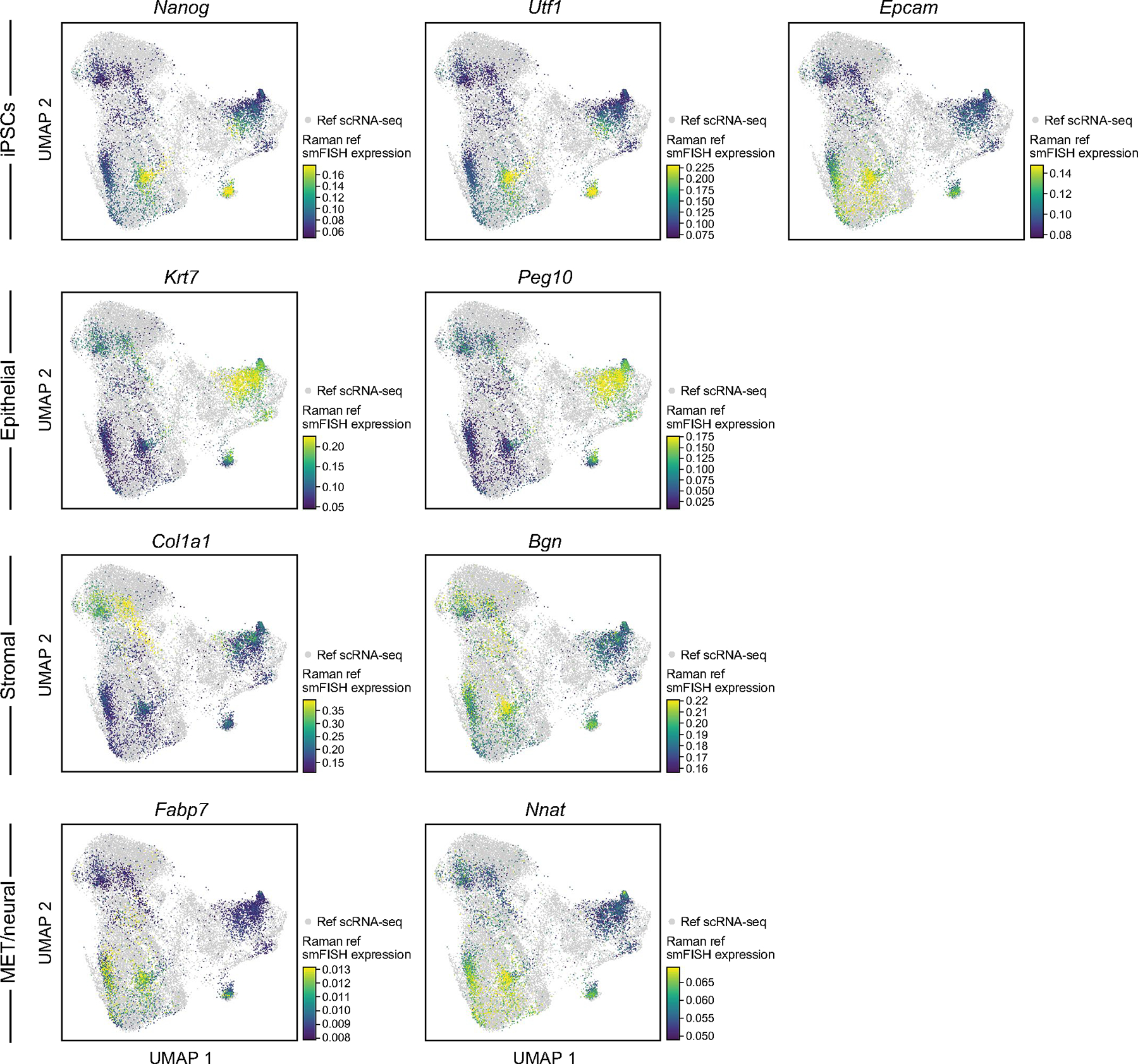
UMAP co-embedding of Raman predicted RNA profiles and measured scRNA-seq profiles (dots) where the Raman cells are colored by smFISH measurement of each of nine anchor genes.

Extended Data Fig. 5 |. Measured and Raman-predicted single cell profiles co-embed well as reflected by scRNA-seq based expression of nine anchor genes.

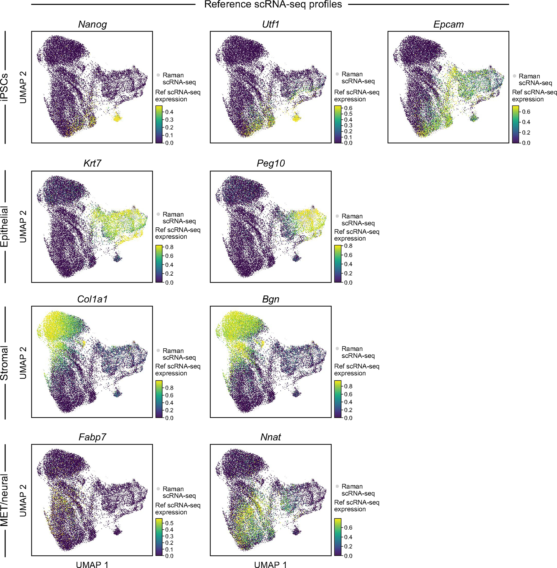
UMAP co-embedding of Raman predicted RNA profiles and measured scRNA-Seq profiles (dots) where the scRNA-seq profiled cells are colored by scRNA-seq measured expression of each of nine anchor genes.

Extended Data Fig. 6 |. Distributions of expression of marker genes based on R2R-predicted profiles.

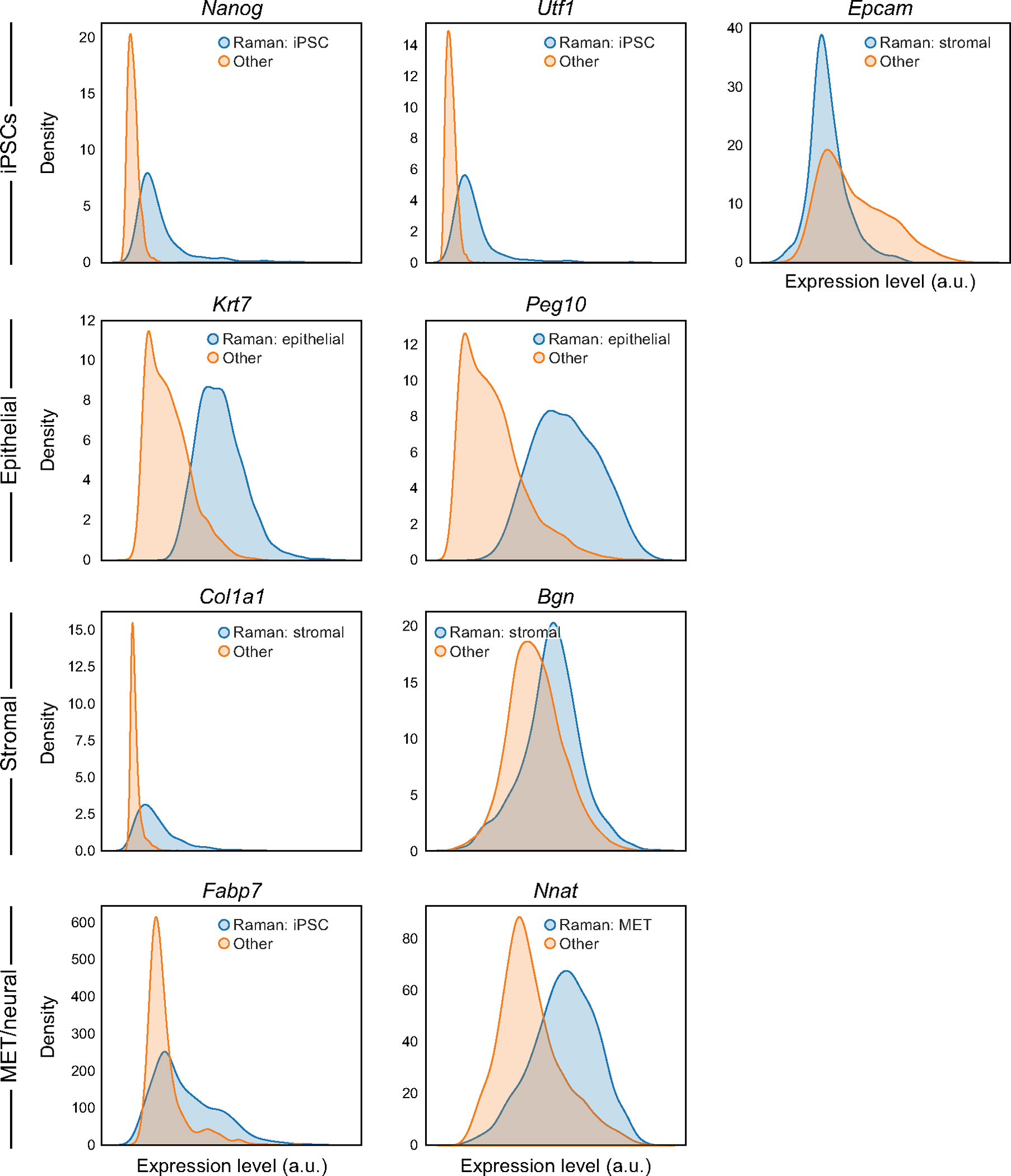
Distributions (density plots) of the predicted expression in Raman2RNA inferred profiles for each marker gene (panel) in its expected corresponding cell type (blue, based on the predicted expression profiles) and all other cells (orange).

Extended Data Fig. 7 |. Distributions of expression of marker genes based on real smFISH profiles.

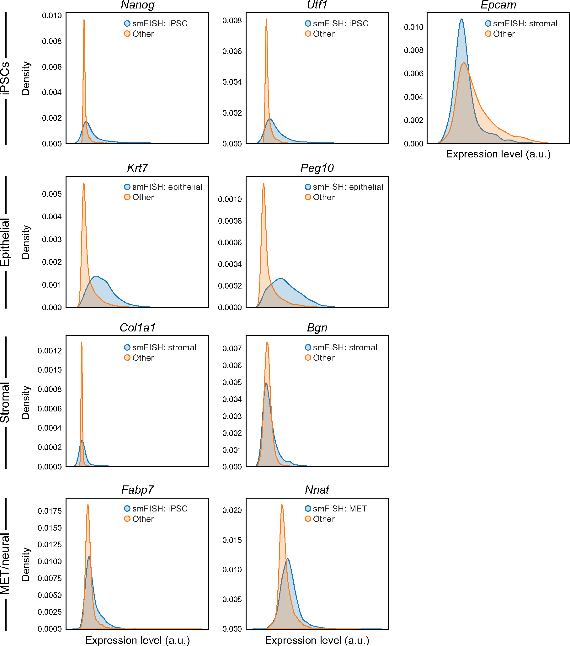
Distributions (density plots) of the real smFISH profiles for each marker gene (panel) in its expected corresponding cell type (blue, based on the R2R predicted expression profiles) and all other cells (orange).

Extended Data Fig. 8 |. Raman spectral feature importance scores for each smFISH anchor gene and its average across all genes for a cell type.

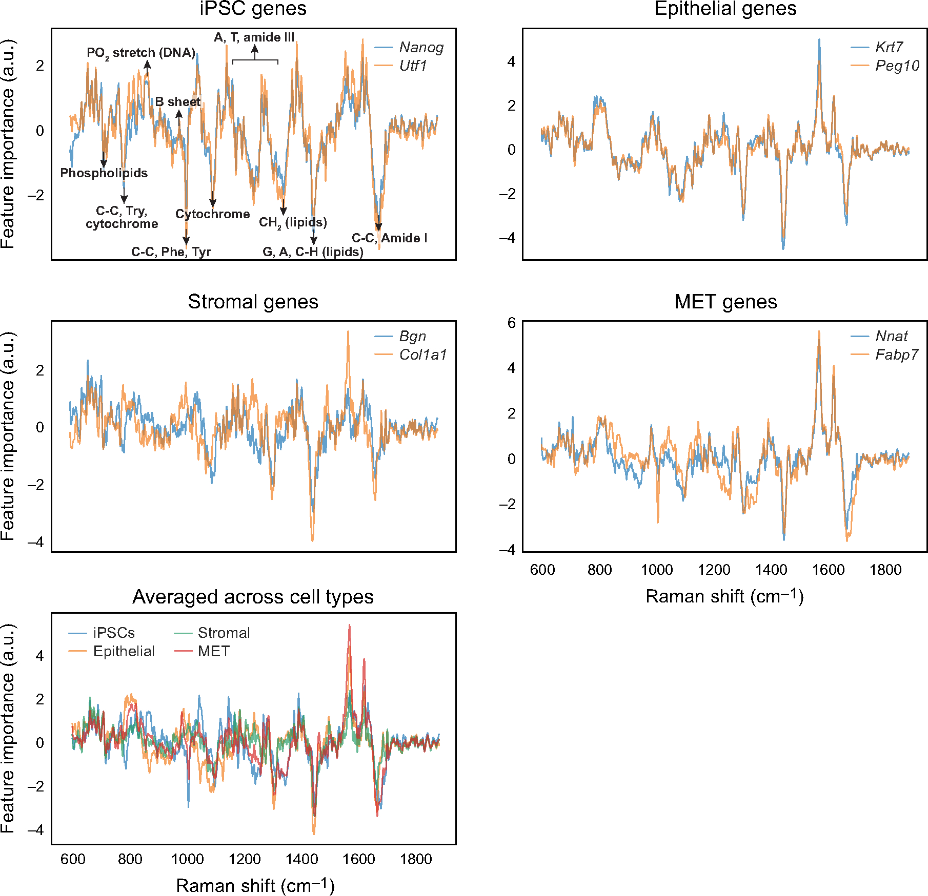
Feature importance scores (y axis) for marker genes of each cell type (top two rows), and for all cell types (bottom row), along the Raman spectrum (x axis). Known signals² are annotated in the top left panel (identical to Fig. 3j).

Extended Data Fig. 9 |. Adversarial autoencoder (AAE) based model for anchor-free generation of scRNA-seq from Raman profiles.

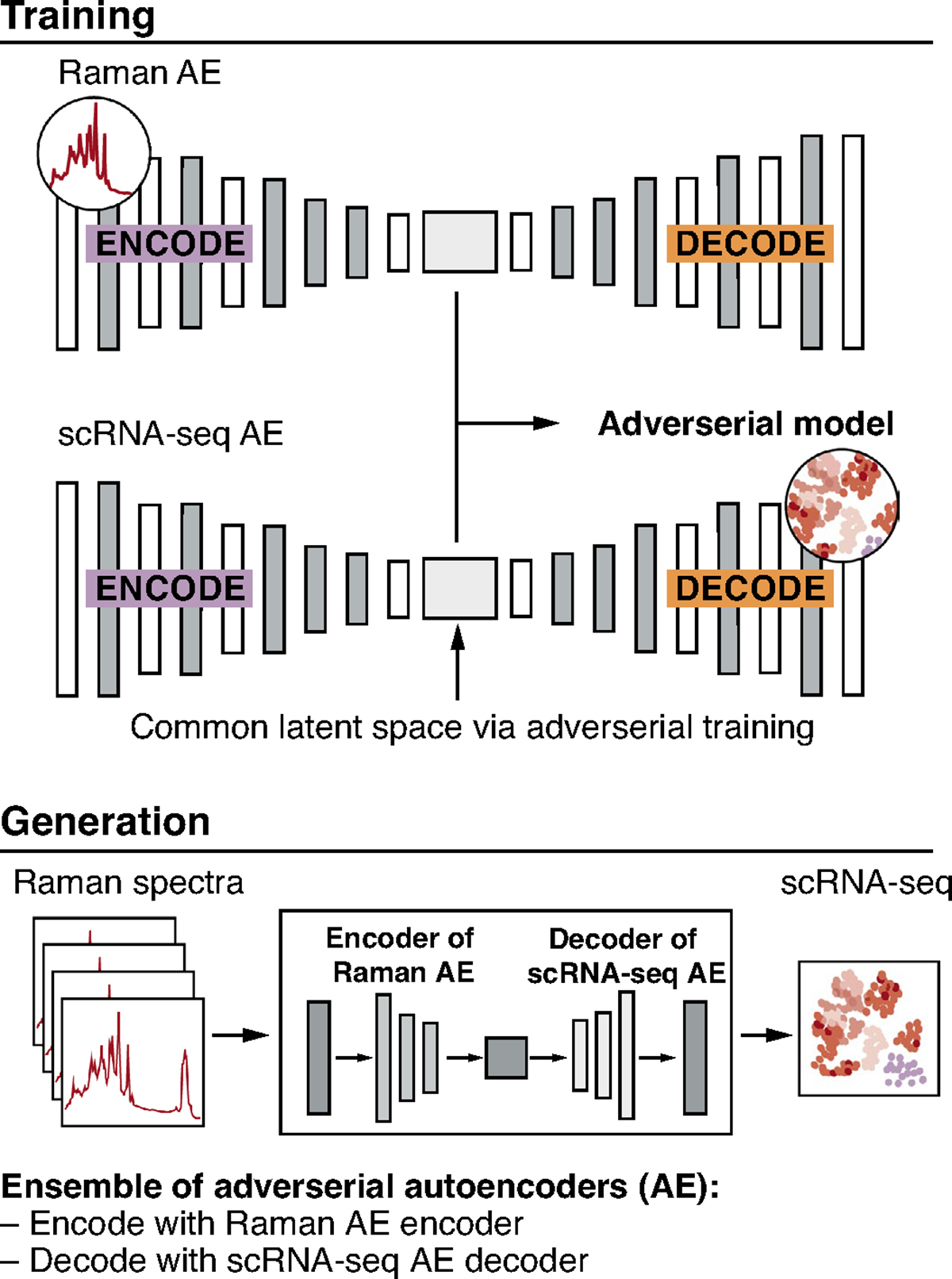
Top: Two autoencoders (AEs) – one for Raman and the other for scRNA-seq – are trained adversarially to learn two indistinguishable latent spaces. Once a common latent space is found, new Raman spectra are encoded using the encoder part of the Raman AE and decoded to scRNA-seq using the decoder part of the scRNA-seq AE (bottom).

Extended Data Fig. 10 |. Anchor-free R2R profiles capture variance in single cell profiles as indicated by co-embedding.

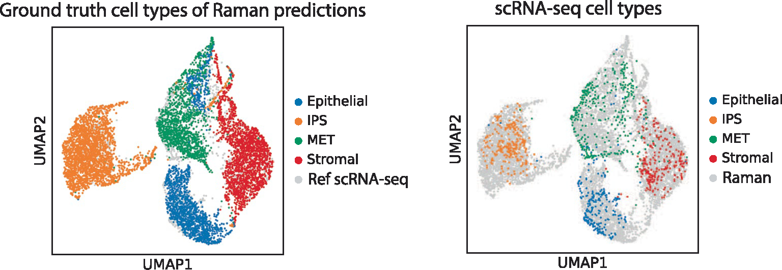
UMAP co-embedding of anchor-free R2R-generated profiles and real scRNA-seq (dots) colored by cell types determined by Tangram label-transfer on smFISH measurements (left, for cells with R2R-generated profiles) or by ground truth scRNA-seq (right, for cells with scRNA-seq profiles).

Data availability

Raw data for the mouse reprogramming scRNA-seq are available for download from NCBI Gene Expression Omnibus (https://www.ncbi.nlm.nih.gov/geo) under project number: GSE122662. mES cell differentiation scRNA-seq data are available publicly²⁰. All other data are available at https://console.cloud.google.com/storage/browser/raman2rna.

References

- 1.Tanay A & Regev A Scaling single-cell genomics from phenomenology to mechanism. Nature 541, 331–338 (2017). [DOI] [PMC free article] [PubMed] [Google Scholar]
- 2.Trapnell C et al. The dynamics and regulators of cell fate decisions are revealed by pseudotemporal ordering of single cells. Nat. Biotechnol. 32, 381–386 (2014). [DOI] [PMC free article] [PubMed] [Google Scholar]
- 3.Schiebinger G et al. Optimal-transport analysis of single-cell gene expression identifies developmental trajectories in reprogramming. Cell 176, 928–943.e22 (2019). [DOI] [PMC free article] [PubMed] [Google Scholar]
- 4.La Manno G et al. RNA velocity of single cells. Nature 560, 494–498 (2018). [DOI] [PMC free article] [PubMed] [Google Scholar]
- 5.Bergen V, Lange M, Peidli S, Wolf FA & Theis FJ Generalizing RNA velocity to transient cell states through dynamical modeling. Nat. Biotechnol. 38, 1408–1414 (2020). [DOI] [PubMed] [Google Scholar]
- 6.Wagner DE & Klein AM Lineage tracing meets single-cell omics: opportunities and challenges. Nat. Rev. Genet. 21, 410–427 (2020). [DOI] [PMC free article] [PubMed] [Google Scholar]
- 7.Gorin G, Fang M, Chari T & Pachter L RNA velocity unraveled. Preprint at bioRxiv 10.1101/2022.02.12.480214 (2022). 2022.02.12.480214. [DOI] [PMC free article] [PubMed] [Google Scholar]
- 8.Rabani M et al. High-resolution sequencing and modeling identifies distinct dynamic RNA regulatory strategies. Cell 159, 1698–1710 (2014). [DOI] [PMC free article] [PubMed] [Google Scholar]
- 9.Wei L et al. Super-multiplex vibrational imaging. Nature 544, 465–470 (2017). [DOI] [PMC free article] [PubMed] [Google Scholar]
- 10.Chen W et al. Live-seq enables temporal transcriptomic recording of single cells. Nature 10.1038/s41586-022-05046-9 (2022). [DOI] [PMC free article] [PubMed] [Google Scholar]
- 11.Kobayashi-Kirschvink KJ et al. Linear regression links transcriptomic data and cellular Raman spectra. Cell Syst. 10.1016/j.cels.2018.05.015 (2018). [DOI] [PubMed] [Google Scholar]
- 12.Singh SP et al. Label-free characterization of ultra violet-radiation-induced changes in skin fibroblasts with Raman spectroscopy and quantitative phase microscopy. Sci. Rep. 7, 10829 (2017). [DOI] [PMC free article] [PubMed] [Google Scholar]
- 13.Ichimura T et al. Visualizing cell state transition using Raman spectroscopy. PLoS ONE 9, e84478 (2014). [DOI] [PMC free article] [PubMed] [Google Scholar]
- 14.Ho C-S et al. Rapid identification of pathogenic bacteria using Raman spectroscopy and deep learning. Nat. Commun. 10, 4927 (2019). [DOI] [PMC free article] [PubMed] [Google Scholar]
- 15.Biancalani T et al. Deep learning and alignment of spatially resolved single-cell transcriptomes with Tangram. Nat. Methods 18, 1352–1362 (2021). [DOI] [PMC free article] [PubMed] [Google Scholar]
- 16.Stadtfeld M, Maherali N, Borkent M & Hochedlinger K A reprogrammable mouse strain from gene-targeted embryonic stem cells. Nat. Methods 7, 53–55 (2010). [DOI] [PMC free article] [PubMed] [Google Scholar]
- 17.Choi HMT et al. Third-generation in situ hybridization chain reaction: multiplexed, quantitative, sensitive, versatile, robust. Development 145, dev165753 (2018). [DOI] [PMC free article] [PubMed] [Google Scholar]
- 18.McInnes L, Healy J, Saul N & Großberger L UMAP: uniform manifold approximation and projection. J. Open Source Softw. 3, 861 (2018). [Google Scholar]
- 19.Germond A, Panina Y, Shiga M, Niioka H & Watanabe TM Following embryonic stem cells, their differentiated progeny, and cell-state changes during iPS reprogramming by Raman spectroscopy. Anal. Chem. 92, 14915–14923 (2020). [DOI] [PubMed] [Google Scholar]
- 20.Semrau S et al. Dynamics of lineage commitment revealed by single-cell transcriptomics of differentiating embryonic stem cells. Nat. Commun. 8, 1096 (2017). [DOI] [PMC free article] [PubMed] [Google Scholar]
- 21.Zhou Y et al. Metascape provides a biologist-oriented resource for the analysis of systems-level datasets. Nat. Commun. 10, 1523 (2019). [DOI] [PMC free article] [PubMed] [Google Scholar]
- 22.Lange M et al. CellRank for directed single-cell fate mapping. Nat. Methods 19, 159–170 (2022). [DOI] [PMC free article] [PubMed] [Google Scholar]
- 23.Li C, Virgilio M, Collins K & Welch JD Multi-omic single-cell velocity models epigenome–transcriptome interactions and improves cell fate prediction. Nat. Biotechnol. 41, 387–398 (2023). [DOI] [PMC free article] [PubMed] [Google Scholar]
- 24.Wu H et al. In vivo lipidomics using single-cell Raman spectroscopy. Proc. Natl Acad. Sci. USA 108, 3809–3814 (2011). [DOI] [PMC free article] [PubMed] [Google Scholar]
- 25.Kunapareddy N, Freyer JP & Mourant JR Raman spectroscopic characterization of necrotic cell death. J. Biomed. Opt. 13, 054002 (2008). [DOI] [PubMed] [Google Scholar]
- 26.Freudiger CW et al. Label-free biomedical imaging with high sensitivity by stimulated Raman scattering microscopy. Science 322, 1857–1861 (2008). [DOI] [PMC free article] [PubMed] [Google Scholar]
- 27.Bai Y et al. Ultrafast chemical imaging by widefield photothermal sensing of infrared absorption. Sci. Adv. 5, eaav7127 (2019). [DOI] [PMC free article] [PubMed] [Google Scholar]
- 28.Tamamitsu M, Toda K, Horisaki R & Ideguchi T Quantitative phase imaging with molecular vibrational sensitivity. Opt. Lett. 44, 3729–3732 (2019). [DOI] [PubMed] [Google Scholar]
- 29.Cleary B, Cong L, Cheung A, Lander ES & Regev A Efficient generation of transcriptomic profiles by random composite measurements. Cell 171, 1424–1436.e18 (2017). [DOI] [PMC free article] [PubMed] [Google Scholar]
- 30.Eng C-HL et al. Transcriptome-scale super-resolved imaging in tissues by RNA seqFISH. Nature 568, 235–239 (2019). [DOI] [PMC free article] [PubMed] [Google Scholar]
- 31.Chen KH, Boettiger AN, Moffitt JR, Wang S & Zhuang X RNA imaging. Spatially resolved, highly multiplexed RNA profiling in single cells. Science 348, aaa6090 (2015). [DOI] [PMC free article] [PubMed] [Google Scholar]
- 32.Wang X et al. Three-dimensional intact-tissue sequencing of single-cell transcriptional states. Science 10.1126/science.aat5691 (2018). [DOI] [PMC free article] [PubMed] [Google Scholar]
- 33.Alon S et al. Expansion sequencing: spatially precise in situ transcriptomics in intact biological systems. Science 371, eaax2656 (2021). [DOI] [PMC free article] [PubMed] [Google Scholar]
- 34.Kang JW, Nguyen FT & Lue N Temporal imaging of live cells by high-speed confocal Raman microscopy. Materials 14, 3732 (2021). [DOI] [PMC free article] [PubMed] [Google Scholar]
- 35.Kang JW, So PTC, Dasari RR & Lim D-K High resolution live cell Raman imaging using subcellular organelle-targeting SERS-sensitive gold nanoparticles with highly narrow intra-nanogap. Nano Lett. 15, 1766–1772 (2015). [DOI] [PMC free article] [PubMed] [Google Scholar]
- 36.Radford A et al. Learning transferable visual models from natural language supervision. In International Conference on Machine Learning 8748–8763 (PMLR, 2021). [Google Scholar]
- 37.Edelstein A, Amodaj N, Hoover K, Vale R & Stuurman N Computer control of microscopes using μManager. Curr. Protoc. Mol. Biol. 10.1002/0471142727.mb1420s92 (2010). [DOI] [PMC free article] [PubMed] [Google Scholar]
- 38.Stuart T et al. Comprehensive integration of single-cell data. Cell 177, 1888–1902.e21 (2019). [DOI] [PMC free article] [PubMed] [Google Scholar]
- 39.Polo JM et al. A molecular roadmap of reprogramming somatic cells into iPS cells. Cell 151, 1617–1632 (2012). [DOI] [PMC free article] [PubMed] [Google Scholar]
- 40.opencv. GitHub; https://github.com/opencv/opencv (2023). [Google Scholar]
- 41.rampy. GitHub; https://github.com/charlesll/rampy (2021). [Google Scholar]
- 42.biomagdsb. GitHub; https://github.com/spreka/biomagdsb (2020). [Google Scholar]
- 43.Prokhorenkova L, Gusev G, Vorobev A, Dorogush AV & Gulin A CatBoost: unbiased boosting with categorical features. In Advances in Neural Information Processing Systems 31 (eds Bengio S et al. ) (NeurIPS, 2018). [Google Scholar]
- 44.Yang KD et al. Multi-domain translation between single-cell imaging and sequencing data using autoencoders. Nat. Commun. 12, 31 (2021). [DOI] [PMC free article] [PubMed] [Google Scholar]
- 45.pegasus. GitHub; https://github.com/klarman-cell-observatory/pegasus (2022). [Google Scholar]
- 46.Wolf FA, Angerer P & Theis FJ SCANPY: large-scale single-cell gene expression data analysis. Genome Biol. 19, 15 (2018). [DOI] [PMC free article] [PubMed] [Google Scholar]
- 47.Ounkomol C, Seshamani S, Maleckar MM, Collman F & Johnson GR Label-free prediction of three-dimensional fluorescence images from transmitted-light microscopy. Nat. Methods 15, 917–920 (2018). [DOI] [PMC free article] [PubMed] [Google Scholar]
- 48.Weigert M, Schmidt U, Haase R, Sugawara K & Myers G Star-convex Polyhedra for 3D object detection and segmentation in microscopy. In Proceedings of the IEEE Winter Conference on Applications of Computer Vision (WACV) 3655–3662 (IEEE, 2020). [Google Scholar]
- 49.napari. GitHub; https://github.com/napari/napari (2022). [Google Scholar]
- 50.Ulicna K, Vallardi G, Charras G & Lowe AR Automated deep lineage tree analysis using a bayesian single cell tracking approach. Front. Comput. Sci. 3, 734559 (2021). [Google Scholar]
- 51.Parekh S, Ziegenhain C, Vieth B, Enard W & Hellmann I zUMIs—a fast and flexible pipeline to process RNA sequencing data with UMIs. Gigascience 7, giy059 (2018). [DOI] [PMC free article] [PubMed] [Google Scholar]
Associated Data
This section collects any data citations, data availability statements, or supplementary materials included in this article.
Supplementary Materials
Data Availability Statement